Estimation procedures for repeated surveys

Roger Grenville Jones

Thesis submitted for the degree of Doctor of Philosophy

at the Australian National University.

E x c e p t w h e r e o t h e r w i s e a c k n o w l e d g e d i n t h e t e x t , t h i s t h e s i s r e p r e s e n t s my o r i g i n a l r e s e a r c h .

This thesis continues work undertaken at the University of Southampton and owes much to the stimulation and inspiration gained from working there with Professor Fred Smith.

To the many friends who have encouraged and coaxed this thesis out of me, I offer my thanks, In particular, Ken and Robyn, Pete and Esther, Vance, Hereward, Katarina and Hugo, Jane, Kay, Paula and Naomi, and Diana who so ably translated my writing to prepare the final manuscript.

Above all, this thesis owes its completion to Maggie whose love, patience, support and friendship have been so important to me

throughout.

The aim of this thesis is to examine the methods of estimation that have been developed for use in sample surveys repeated at regular intervals, with particular emphasis on the time series methods that have recently been proposed.

The practice of surveying a population at regular intervals, to provide timely estimates of characteristics changing over time and the effects of changing conditions, have been of interest throughout the relatively short history of the sample survey method. As long ago as 1942, Jessen showed that by retaining the same sample units from one survey to the next, an improved population estimate could be derived, the gain in efficiency being due to the correlation evident between responses obtained from the same individual unit on different occasions. This idea led to the wider use of overlapping samples in repeated surveys and the development of more general estimates to make efficient use of the overlapping design.

While the correlation between responses given by individual units in the population was accepted and used, the population

characteristic being estimated was assumed to be a fixed value. Any correlation between them over time is then ignored. This rather anamolous situation was pointed out by Blight and Scott (1973) and estimation procedures have since been developed which incorporate the stochastic properties of the population characteristic into the

the theory is not new, but the presentation in this form clarifies the relationships between the various estimates and indicates possible extensions to the existing methods.

One of the factors effecting the efficiency of the time series estimation methods is the form of unbiased estimate on which they are based. Where a rotation design with partial overlap of sampling units is used, unbiased estimates may be derived using data from the current sample only, or composite estimates employed to reduce the sampling variance. Using a one-level rotation design, the effect of this choice is examined in Chapter 2.

In Chapter 3, a stepwise regression estimation procedure is proposed as an alternative to the signal extraction method suggested by Scott and Smith (1974). Using the method of linear differencing, the properties of both estimates are examined for stationary and non­ stationary series, and useful theoretical and empirical results

presented.

The results of these two chapters provide the necessary

CONTENTS

ACKNOWLEDGEMENTS

ABSTRACT

CHAPTER 1. THEORY OF ESTIMATION FOR REPEATED SURVEYS

1.1 Introduction 1.2 Sample Design

1.3 Minimum Variance Linear Unbiased Estiamtors (MVLUE)

1.4 Best Linear Unbiased Estimators - Parameters with Zero Mean 1.5 Best Linear Unbiased Estimators - Parameters with Non-Zero Mean 1.6 Estimation of Dispersion Matrices

CHAPTER 2. EFFICIENCY OF BLU ESTIMATION

2.1 Introduction

2.2 Unbiased Estimation in One-Level Rotation Schemes 2.3 BLU Estimation of 6(h) - Known Mean

3.2 Stepwise Regression Estimation Method

3.3 Stepwise Regression Estimates for Stationary Series

3.4 Stepwise Regression Estimates for Series Requiring

Non-Seasonal Differencing

3.5 Stepwise Regression Estimates for Seasonal Series

THEORY OF ESTIMATION FOR REPEATED SURVEYS

1.1 Introduction

’When a population is subject to change, a single survey will only yield information about the properties of that population on a given occasion. If the changes in the population values are to be examined, the survey will have to be repeated on several occasions.' (Patterson, 1950).

As confidence in survey methods has increased, the use of sample surveys conducted at regular intervals for the collection of

important series of data has become common practice. In Australia, for example, the majority of data collections undertaken by the Australian Bureau of Statistics are periodic surveys run on a monthly, quarterly or annual basis, covering such varied topics as the volume of imports and exports, the level of retail trade,

building activity, capital expenditure, labour force characteristics and so on. Similar surveys are, and have been for many years,

carried out by government agencies throughout the world.

that have occurred between periods such as between successive months, from the corresponding month a year ago, and at other intervals. The results of a number of surveys might also be aggregated, allowing quarterly, half-yearly or yearly totals to be derived from a monthly survey.

In this chapter, the sample designs and estimation procedures that have been developed for repeated surveys are reviewed. Sampling on successive occasions involves a number of problems in theory and in practical survey design and the method of rotation sampling which has been devised to meet these problems is described in Section 1.2. The method of minimum variance linear unbiased estimation implicit in the work of Patterson (1950), Bershad (1952, 1953) and Eckler (1955) but developed in its most general form by Gurney and Daly (1965) is presented in Section 1.3. The recent developments by Blight and Scott (1973), Scott and Smith (1974) and Scott, Smith and Jones (1977) to allow stochastic variation in the parameters being estimated are unified and extended using least squares theory in Section 1.4, and the extension of these results to allow for certain types of non-stationarity is given in Section 1.5.

1.2 Sample Design

(1) a new sample on each occasion;

(2) a fixed sample or panel, used on all occasions; (3) a partial replacement of units on each occasion.

If the efficiency of unbiased estimates of means or totals is the criterion used, the choice of one or other of the above options is complicated by the need to estimate multiple statistics. As

Cochran (1963) for example points out, because there is nearly always a positive correlation between the measurements on the same unit on different occasions, option (1) is best for estimating the average or aggregate over a number of periods, option (2) is best for

estimating change, and for current estimates, option (3) may be the best alternative.

Apart from the criterion of efficiency of unbiased estimates, there are often practical considerations favouring option (3).

Steinberg (1953), describing the sampling scheme used in the Current Population Survey conducted monthly by the US Bureau of the Census

comments;

’It has been found that virtually all respondents can be expected to supply information for several months without creating any administrative problem by refusing to cooperate. However, keeping the same household on for a considerable longer

time would result in higher refusal rates or complaints and requests to be dropped from the panel. Once the decision is reached that it is necessary to have a fresh sample of

staggered basis. Substantial costs are involved in introducing

a set of households for the first time into the sample. For

example, about 5 minutes more is required to enumerate a

household for the first month that it is in the sample than in

succeeding months. Therefore, it is desirable to have only some

of the new households come into the sample at any one time so as to equalise the workload over a number of months.'

Rotation sampling is the term generally used to describe the method by which some units are retained from one survey to the next

and some new units added. In these designs, the sample on each

occasion consists of a number of similar subsamples or rotation groups, with the sample units in a particular subsample entering and leaving the sampling scheme at the same time.

As a simple illustration of a rotation design, consider a single-stage sample in which one quarter of the units are to be

replaced by a new selection on each occasion. The sample on occasion

h, s(h) say, is then made up of four similar subsamples s^(h), 82(h), s^(h) and s^(h) where s^(h) contains new sample units, 82(h) contains

units included on the last occasion, Sß(h) contains units included on the last two occasions, and s^(h) contains units which have been

included for the last three occasions. The sample design may then be

described by the following pattern:

s ^(h) s2 (h)

s ^ h - 1 )

s^Ch) s^(h)

s 2(h - 1) s 2(h-1) s^(h-l)

Each row represents the sample on a particular occasion and each column represents a particular subsample moving through the sampling scheme over four surveys. The monthly Labour Force Survey conducted by the Australian Bureau of Statistics uses this type of rotation scheme on the households selected as final-stage sample units but with a one-eighth rotation.

More complicated rotation patterns can be used, as for example in the US Bureau of the Census' Current Population Survey (Steinberg, 1953; Hansen et at , 1955; Hanson, 1978), where each sample comprises eight subsamples with a rotation pattern which retains units for four months, drops them out for the next eight months, and brings them back into sample for a second four months before dropping them out completely. In this way, six of the eight subsamples for any month are in the sample for the previous month and four are also in the sample for the same month one year ago.

A different kind of rotation design, called two-level rotation sampling, can be used when respondents can be expected to reliably recall information from a previous occasion. In this design, units are not retained from one survey to the next, but a new sample is selected on each occasion which reports both for the current occasion and for the previous occasion. The scheme may be depicted by the pattern:

s 1 (h)

s0 (h-l) s1(h— 1)

where SqOi-I) denotes the responses obtained at time h about time h-1 from the sample respondents in s^(h). This design is used in

particular in the US Bureau of the Census’ Retail Trade Surveys and has received considerable attention in the literature (Bershad, 1952,

1953; Woodruff, 1959; Wolter et al, 1976; Wolter, 1979).

The efficiency of rotation designs is achieved through the

correlations between responses obtained on different occasions. If a single-stage sample design is used on each occasion, responses from different units will in general be taken as independent measurements and thus correlation between measurements occurs only when the same units are observed on different occasions.

The situation for two-stage surveys, and more generally for multi-stage surveys, is more complex since the overlap can come from any stage of sampling. In this case, measurements from different clusters are in general assumed to be independent while those within the same cluster are correlated. Overlap of sample units from survey to survey may be achieved:

(a) by retaining the same clusters, and using one of the single-stage designs above within each cluster; or

(b) by rotating whole clusters.

However, when all the sample units within a cluster are treated identically, either all being retained or all replaced, it is

are rotated within each cluster, correlation between measurements occurs not only when the same unit is observed on different occasions but also when different units within a cluster are observed either on the same occasion or on different occasions.

1.3 Minimum Variance Linear Unbiased Estimators (MVLUE)

The general problem of obtaining MVLUE for repeated surveys was first solved by Gurney and Daly (1965), although the fundamental ideas were implicit in the earlier work of Jessen (1942) and Patterson (1950). Their method involved the use of Hilbert space theory and was unnecessarily complex. The results are readily

obtained by least squares (Jones, 1975; see also Jones, 1980; Wolter, 1979).

Consider a sample survey which is carried out on h occasions, and let 9(t) , t = l,2,...,h denote the value of the population mean on each occasion. Let x^(t) be an unbiased estimate of 9(t) based on the ith. rotation group in the sample at time t, and let X^ be the vector of all these estimates from the h surveys. Since the estimates x^(t) are unbiased, we can write

x (t) = 0(t) + e.(t), i = 1,2,...; t = 1,2,...,h (1.3.1)

where e^(t) is the sampling error associated with x^(t). Combining all the equations (1.3.1) into matrix form gives

where ( 0(h), 0 ( h - l 9(1)) is the vector of population values;

U is a design matrix of 0's and l's which selects the

appropriate element of 0^ ; and

is an error vector with mean zero and variance var ( e, ) = K say.

h e

Then (assuming inverses exist) generalised least squares gives the of 0 given X^ as

MVLUE

G^d) = (U^K^U) 1 I^K^Xb (1.3.3)

I ^

and the variance of any linear combination £ G^( 1) is

T ~ T T -1 -1

var(£ e^(l)) = £ (ü K Ü) £ (1.3.4)

Results for the two sample case (Jessen, 1942; Singh, 1968; and many others) are easily seen to be special cases of these results as are the more general results of Patterson (1950) and Eckler (1955). A recent application of these results to the two-level rotation

scheme is given by Wolter (1979).

A

Note that 0.(1) is the MVLUE among the class of estimators

h

which are linear in the x^(t) rather than in the observations on the

individual sample units. More precisely, 0.(1) is the MVLUE under

h

the model (1.3.1). No assumptions are then necessary about the

sample selection procedure or the forms of the x^(t), these being

simple random sampling without replacement from an infinite

population, is a sufficient statistic for (Patterson 1950; Eckler, 1955). More generally, sample selection procedures and the method by which estimates are calculated from the sample data are taken as given, and interest then centres on the implications of rotating or retaining the sample rather than selecting a new sample on each occasion. The additional information due to rotation is then encapsulated by the rotation group estimates. Taking this view, we consider linear estimates based only on the rotation group estimates x^(t) throughout. Because these estimates only use data from a single survey, they are sometimes called simple or elementary estimates.

The limitation that x^(t) be unbiased can be relaxed by

incorporating the bias into 0(t) or equivalently extending the model (1.3.1) to the form

x , (t ) = 9(t) + b(t) + e.(t)

l l

1.4 Best Linear Unbiased Estimators - Parameters with zero nean The estimates obtained from surveys conducted at regular

intervals will often be considered as observations in a time series

and be subject to the techniques of time series analysis. For

example, estimates from a monthly or quarterly series may be adjusted to take account of seasonal effects and a trend fitted in order to

obtain forecasts of future values. Implicit in this form of analysis

is the idea that the population values are in some way related over time.

In the classical sampling theory approach of the previous

section, estimates which are unbiased in respect only of the sampling probabilities are the principal aim and the population values being

estimated are taken as fixed. Thus any relationship that might exist

between successive values of the population parameters

9(1),9(2),...,9(h) is ignored completely. Any use that is made of

time series analysis is based only on the final estimates produced from each survey and the effects of the survey design on the time series properties of the estimates is then ignored.

Recent work on estimation for repeated surveys has sought to incorporate the sample design and time series aspects into a single

estimation procedure. In this approach, the series of population

values {©(t): t =l,2,...,h } is regarded as one realisation of a

stochastic process or, in the terminology of sampling theory, as the values obtained from a population drawn at random from an infinite

superpopulation. The efficiency of an estimator is then no longer

efficiency over all populations in the superpopulation.

To be specific let

E

T

1 ^ is unbiased and has minimum variance only in respect of the sampling expectation E, © being considered a fixed parameter. In

h

this section, © is a random variable (with mean zero) and the 'best’ h

estimator is determined in respect of the joint expectation

EE,

particular, we require a linear estimator L of £ ^ such that

E E

and

EE

*

V

This will be termed the best linear unbiased estimator (BLUE). Note that if the sampling-unbiased condition is imposed, then the BLUE

T 2

reverts to the MVLUE. The quantity £’E(L -

l

EE

approach are presented by Scott, Smith and Jones (1977) and Dagsvik (1978).

In this section, the BLUE are derived using the theory of

stochastic least squares. This approach leads to a generalisation of

the results of Blight and Scott, and the relationship between their results, those of Scott and Smith, and the MVLUE of Gurney and Daly are clarified.

Suppose that the vector of population parameters © in equation h

(1.3.2) is assumed to be a random variable with mean zero and

dispersion matrix V a r ( 0 ) . Then the best linear unbiased estimator

h

T T*

l ej^(2) of I is given immediately by (Rao, 1973, p234)

(1.4.1)

with

(1.4.2)

An alternative derivation of these results is the following.

Firstly, the MVLUE 0 ( 1 ) is calculated as in (1.3.3). Then we may

h write

ehU) - ^ + eh(i)

e, ( 1 ) = (UTK 1ü)

h e ( 1 . 4 . 4 )

and

v a r ( e h ( l ) ) = ( D ^ K ^ U ) 1 ( 1 . 4 . 5 )

Then a p p l y i n g s t o c h a s t i c l e a s t s q u a r e s t h e o r y t o ( 1 . 4 . 3 ) g i v e s t h e r e s u l t :

g i v e s ( 1 . 4 . 1 ) and ( 1 . 4 . 2 ) f o l l o w s s i m i l a r l y .

As e s t i m a t o r o f t h i s f orm was d e r i v e d by B l i g h t and S c o t t ( 1 9 7 3 )

a u t o r e g r e s s i v e m o d e l . T h e i r a p p r o a c h gave r e c u r s i v e e q u a t i o n s f o r t h e e s t i m a t o r s of t h e c u r r e n t l e v e l 0(h) and most r e c e n t c h a n ge

0(h) - 0(h - 1) . T h e s e e q u a t i o n s a r e , i n f a c t , j u s t t h e r e c u r s i v e u p d a t i n g e q u a t i o n s o b t a i n e d u s i n g t h e Kalman f i l t e r ( s e e , f o r

e x a m p l e , Duncan and H o r n , 1 9 7 2 ) , and t h i s method c o u l d be u s e d more g e n e r a l l y i n s i t u a t i o n s wh e re an o b s e r v a t i o n e q u a t i o n and a s t a t e t r a n s i t i o n e q u a t i o n can be d e f i n e d . A l t h o u g h r e c u r s i v e e q u a t i o n s c a n be u s e f u l i n r e d u c i n g t h e c o m p u t a t i o n b u r d e n o f t h e e s t i m a t i o n

p r o c e s s , B l i g h t and S c o t t r e p o r t e d t h a t f o r h i g h e r a u t o r e g r e s s i v e m od el s t h e y wer e ' v e r y much more c o m p l i c a t e d ' , and t h e r e i s t h e

A

further difficulty that the state transition equation and observation equation will, in general, be unknown.

In order to overcome the problems of model specification inherent in this approach, Scott and Smith (1974) developed an

alternative procedure based on the theory of signal extraction in the presence of stationary noise. Taking y(h) as 'the standard sample survey estimate of 9(h) based on the sample at time t alone, and suppose that y(h) is approximately unbiased' they write

zero and dispersion matrix K g which is assumed to be known or at least estimable from the survey data. Then stochastic least squares

y(h) = 9(h) + e(h)

or, in matrix form

Yh ■ 1 + %

where Y hT = (y(h),...,y(1)), ehT = (e(h),...,e(1)) and eh has mean

T gives the BLUE of £ Q as

(1.4.7)

with

Using the identity (Rao, 1973, p33)

« f

1

=

Var^))’1^

= K - K Var (Yu )_1 K

e e h e

and substituting in (1.4.7) and (1.4.8) gives

tT ^ ( 3 ) = t \ - t \ var(Yh f h h

T ^

1 (Yh "

V

and

MSE (£T ^(3)) = lT (Ke-KeVar(Yh ) !K )£

= £TMSE(eh )Jl (1.4.10)

This, in matrix form, is the estimator proposed by Scott and Smith (1974). The signal extraction approach they used simply provides a procedure for evaluating Var(Y^) ^ when the number of surveys h is assumed to be large and y(t) stationary.

Note that to restrict y(h) to the standard sample survey

practice, a method of estimating K g and Var(Y^) In particular, the fully efficient linear estimator is obtained by using the MVLUE

A

0,(1) in place of Yh as shown in equations (1.4.1) - (1.4.5).

h ri

1.5 Best Linear Unbiased Estimators - Parameters with non-zero mean In deriving the results of section 1.4, it has been assumed that the vector of population means ^ has mean zero, a situation which is

very unlikely to hold in practice. If the mean £”(© ) = y were known,

h

T /v T

the estimator £ 6^(3) = L Y^ of 0 * 4 . 9 ) is simply adjusted to the T

form a + L Y^ where

T T

a = y £ - y L

However, if the mean is completely unknown, the best estimate is T a

given by taking a = 0 and using £ €^(1) , the MVLUE (Rao, 1973). Thus if the time series properties of (9(t)} are to be used in the

estimation process, some assumption about the form of the unknown

mean vector must be made. Two possible approaches are considered

below.

One approach, used in the signal extraction method (Scott, Smith and Jones, 1977), is to assume that {0(t)} is a member of the class of autoregressive integrated moving average (ARIMA) processes (Box

and Jenkins, 1970). (B(t)} is then reduced to stationarity about a

Assume t h e n t h a t mean of t h e p r o c e s s { 0 ( 0 } c a n be r e d u c e d t o z e r o by l i n e a r d i f f e r e n c i n g and l e t d e n o t e t h e v e c t o r of d i f f e r e n c e d t e r m s wh e r e A i s t h e a p p r o p r i a t e d i f f e r e n c i n g o p e r a t o r . We can t h e n c o n s i d e r j o i n t l y t h e e q u a t i o n s

%

AG + T h h

S i n c e t h e mean of ©, i s unknown, t h e BLUE 0 ( 3 ) i s g i v e n by t r e a t i n g

h h

© as a f i x e d p a r a m e t e r and a p p l y i n g g e n e r a l i s e d l e a s t s q u a r e s , h

Hence

^ ( 3 ) = ( i f 1 + ATV a r ( ^ ) 1 A) 1Kg ^

( V Ke AT( * e AT + V a r ( ^ ) ) '1® e ) K O h

Y - K A1 V a r ( M ) ~ 1 A?

h e h h

0 .5.1)

s i n c e A = V ar ( Ae^) and V a r ( T^) = V ar ( A0^) . S i m i l a r l y

M S E ( ^ ( 3 ) ) = K - Ke ATV a r ( M h ) 1 AKg ( 1 . 5 . 2 )

An a l t e r n a t i v e a p p r o a c h i s t o as sume t h a t t h e mean ca n be e x p r e s s e d as a l i n e a r c o m b i n a t i o n Ha of unknown f i x e d p a r a m e t e r s

a = ( a , a , . . . , a ) ,wh e r e H i s an h * p mat r i x o f s p e c i f i e d

U 1 p

c o n s t a n t s . Then Y = 0 - Ha h a s z e r o mean and h h

Yh = Ha + [ I h

A p p l y i n g t h e r e s u l t s f ro m H a r v i l l e ( 1 9 7 6 ) t h e n g i v e s

a = (HTVar(Y, ) - 1 H) _ 1HTV ar (Y u ) - 1 Yu

h h h

\ = V a r ( ^ ) V a r ( Y h ) _ 1 (Yh - Hc0

= (Yh - Ha) - Ke V ar (Y h ) _ 1 (Yh - Bet) and h e n c e

€ ^ ( 3 ) = Yh - Ke V ar (Y h ) _ 1 (Yh - Hot) ( 1 . 5 . 3 )

w i t h

MS E( € ^( 3) ) = Kg - Ke Va r (Yh ) " 1Ke

+ K V ar (Yu ) " 1H(HTVa r( Yu ) " 1H) “ 1HTVa r(Yu ) " 1K ( 1 . 5 . 4 )

e h h h e

A

Thus a i s A i t k e n ' s g e n e r a l i s e d l e a s t s q u a r e e s t i m a t o r ( A i t k e n , 1935) and e s t i m a t e s of a and V ar ( Y ^ ) ^ c a n be o b t a i n e d by i t e r a t i v e m e t h o d s ( Dhr ymes , 1 9 7 1 ) .

N ot e t h a t i f t h e t r e n d H a c a n be d i f f e r e n c e d t o z e r o so t h a t T T

AH = 0 , o r t r a n s p o s i n g , H A = 0 , t h e n ( R a o, 1973, p77)

Var (Y ) ~ 1 = AT ( Ä ^ a r ( Y u ) A1 ) ” 1 A + Var(Y, ) _ 1 H(HTVar(Y, ) " 1H ) ~ 1HTVar(Y, ) _1

h h h h h

1.6 Estimation of the Dispersion Matrices

Both MVLU and BLU estimation require knowledge of the sampling

variance-covariance pattern of the elementary estimates x^(t) (K^) or a

T -1

linear combination of them ( U K U or K ) . This will depend on the

e e

sample design, the correlation between the observations, and the form of

the estimate used. If there is overlap of sample units at any sampling

stage, data from past surveys must be retained in a manner which allows matching either of the units themselves or of some aggregation of these

units which allows the required covariances to be calculated. Since this

process is undoubtedly increasingly costly as the number of observations retained and matched increases, estimation procedures which, though less precise, limit the storage requirements may be preferred.

If the elementary estimates x^(t) based on aggregations of

observations from each rotation group in each survey can be assumed to be uncorrelated for different rotation groups, the random group method of estimating variances (Hansen, Hurvitz and Madow, 1953, p440) can be

extended directly to include covariance estimates. For example, if g

rotation groups are used, each group being retained in the survey for g consecutive occasions before being replaced, we can write

x.(t) = 0(t) + e.(t) ,

l l

-1 g

y(t) = g I x i (t) = 0(t) + e(t) ,

c. (e(t)) i f j = ( i - k ) and k < i g

E ( Gi(t),e (t - k)) =

0 otherwise

where (i - k) ranges through the values i , i - l,...,l,g, g - 1 ,...,g , ... as

O

k increases with the rotation subsample s^(t) on which x^(t) is based entering the sample for the first time when (i - k) = 1.

O

Then it follows that

r S

E{ l (xi (t) - y(t))(x^i_k ^ (t-k)-y(t-k)) } = g(g-l)c^CeCt)) (1.6.1)

1 g

where ck (e(t)) = E(e(t),e(t-k)) = g_2(g-k)ck (e (t)),k=0,1,...,g-l and ck (e(t)) =ck (e(t)) = 0 for k > g. Further random subdivision of g

rotation groups into m subgroups giving g ’ = mg random subgroups improves the precision of the estimate obtained from (1.6.1) with g' replacing g. In addition, if e(t) is stationary, the estimates can be averaged over time.

This method can be used with simple random and p.p.s. (probability proportional to size with replacement) sample designs, and with similar stratified designs provided that each rotation group (and subgroup)

contains the appropriate representation from each stratum. It can also be applied to multi-stage designs where the primary sampling units are

selected as above and

(ii) p.s.u.’s are retained indefinitely, and all sampling units selected within a p.s.u. at all subsequent stages rotate in and out together.

In this second case however, it is necessary to modify our approach to take account of the correlation resulting from the retention of

p.s.u.’s. Under the usual hierarchical model, we set

e.(t) = b . (t) + w.(t)

i l l

where

E(b.(t), b.(t- k)) = c (b (t )) if i=j

i J k

0 otherwise

and

E(wi (t), w_.(t - k)) = c^CwCt)) if j = (i-k) and k < i

0 otherwise

Thus b^(t) represents the effect on x^(t) of between clusters variation and w^(t) that between units within clusters. The estimate (1.6.1) for c^(e(t)) still applies, but now for k > g ,

c^ (e (t ) ) = g 2 c^CeCt)) = g 2 c^(b(t))

need no longer be zero, and for 0 < k < g, c^(b(t)) and c^.(w(t)) must be estimated separately if an estimate of is required. As above

of c^CwCt)), 0 < k < g, is given by

g

c^CwCt)) = l (xi (t) - y(t))(x i_k (t) - y (t-k))

£ E (xi (t) - y^t ))(x (i_ic) (t-k) - y( t-k))

1

g

and c^(b(t)) is given by substitution in the equation

g2 ck (e(t)) = gc^(b(t)) + (g-k) (w(t ))

The more common form of multi-stage design however is one in which p.s.u.'s are selected and retained indefinitely, with a partial

replacement of units selected within each p.s.u. on each occasion. The

elementary estimates are then no longer uncorrelated and the random group

method is inappropriate. With this type of design, ultimate clusters can

serve as an effective unit for variance-covariance estimation.

An ultimate cluster (Hansen, Hurvitz and Madow, 1953) consists of all the final stage sample units selected in a p.s.u., and ultimate cluster variance and covariance estimates use only the unbiased estimates obtained

from each of the selected p.s.u.’s. Suppose that the population contains

the population characteristic based on the j 'th sample p.s.u., and y(t)

the usual total sample estimate. If the sample is self-weighting, then a

ck (e(t))

m

£ (p.(t) - y(t))(p.(t-k) - y(t-k))

3 3

m(m-l)

Similarly, if x^(t) is the rotation group estimate, with sampling error

e^(t) , and P-jj(t) is the j f th p.s.u. sample estimate based only on the

units in the i'th rotation group, the covariance c (e.(t)) is estimated

K. 1

by

ak (£i(t))

(p..(t) - x.(t))(p..(t-k) - x.(t-k)) i.1_______i______U ________ I_____

m ( m - 1)

More generally, ultimate cluster estimates can be made when the sample is

not self-weighting and with stratified samples. Details of the

modifications required are given in Hansen, Hurvitz and Madow (1953, p399) for variance estimates, and covariance estimation formulae follow with obvious modifications.

The second estimation problem is the inverse of the autocovariance

matrix Var(Y^) * or alternatively Var(G^) ^ . The first task is to

estimate or eliminate the mean in the series y(t) , perhaps using

generalised least squares or linear differencing as indicated in the previous section, although other approaches such as the X-ll Program

developed by the U.S. Bureau of Census (1967) might be used. If the

generalised least squares approach is used, Var(Y^) ^ and the mean Ha are

estimated simultaneously.

If the number of surveys in the series is large and y(t) can be

reduced to stationarity by linear differencing, then the auto-covariance pattern of the differenced series can be estimated and a model fitted by

Scott and Smith (1974) and Scott, Smith and Jones (1977) is then the most

appropriate. It should be noted however that non-stationarity of the

variance-covariance estimates can arise both through the signal process

{0(t)} and through the error process (e(t)l . For example, if is the

MVLUE 0^(1) , the error process e^(l) with dispersion matrix

T -1 -1

(U U) is not generally second-order stationary. Heteroscedasticity

of sampling variance with respect to changes in the level of the

population parameters also occurs frequently with survey data. It may

therefore be necessary to transform the unbiased estimates and calculate appropriate sampling variance and covariance estimates for the transformed data before using this approach.

A further difficulty with BLU estimation, and with the model fitting approach in particular, 'is that the number of observations in time is

usually too small at present. Clearly, no complete time series models can

be fitted to short runs of data.' (Scott and Smith, 1973). In such

cases, estimates of the autocorrelation pattern can be quite seriously

biased, highly correlated and highly variable. While this will be a

problem with both the generalised least squares and model fitting approach, the former has the advantage that its reliance on these estimates can be limited by restricting the number to be used in the

estimation process. As Scott and Smith again comment; 'since we are only

concerned with estimation of the parameter 0(t) and not with an

explanation of the underlying stochastic phenomenon, much of the gains in variance terms due to fitting the 'best' model can be obtained by fitting a simple model ....Failure to fit such a model is wasting all the

CHAPTER 2

EFFICIENCY OF BLU ESTIMATION

2.1 Int roduction

Implementation of the BLU estimation theory presented in Chapter 1 can be considered to involve three stages:

1. unbiased estimation of the vector 0, of population

h parameters, giving a vector Y say;

h

2. elimination of the mean or trend E(Y ) = (0 ) ;

h h

3. estimation of the vector 0 - (0 ) based on the detrended

h h

vector of unbiased estimates Y, - E(Y, ) .

h n

Fully efficient BLU estimation can only be achieved when the

vector Y, of unbiased estimates is the MVLUE 0, (1) of 0, . The

h h h

information loss from using less efficient unbiased estimates cannot

be recovered during subsequent stages. This is not to say however

that the reduction in variance achieved by MVLUE will carry through to give correspondingly important reductions in the MSE of the BLUE.

MVLUE are in any case rarely used in practice. The vector

0,(1) comprises estimates for all previous occasions revised in the h

light of more recent data and there is little interest in revising

already published results. Interest will usually centre only on the

has occured between the current occasion and recent past occasions. A second factor mitigating against the use of MVLUE is their dependence on knowledge of the covariance structure of each item of interest. When the large number of estimates required from each survey is considered, the additional computation costs usually heavily outweigh the potential gains of extra efficiency. Thus simpler 'composite' estimators have been developed (Gurney and Daly, 1965, for example) whose form is independent of the specific

covariance pattern of any one variable and yet still give most of the gains, in terms of reduced variance, of the MVLUE. One important estimator of this form is that used in the US Bureau of Census'

Current Population Survey (Hansen gt al , 1955; Rao and Graham, 1964). The effect of eliminating the trend on the efficiency of BLU estimation can only be assessed with respect to a particular model of the trend component, the simplest being that of a polynomial in the time element t with fixed coefficients, p(t) say. The current parameter value 9(t) may then be considered in the form

0(t) = p(t) + iKt)

known. In general of course, different polynomials will be used to represent different parts of the series rather than attempting to fit one polynomial to the whole series.

Here we will consider only the limiting case and assume that the

trend in known. Knowledge of the efficiency of BLU estimation in

this case is central to the general case where the mean must be estimated, with some loss of efficiency as a consequence.

Throughout this chapter, we adopt the standard assumption, made in most of the literature on unbiased estimation for repeated

surveys, of an exponential correlation pattern between observations

on the same unit on different occasions. We can then draw on the

results of Patterson (1950) and Cochran (1953) for details of the MVLUE and on the study by Rao and Graham (1964) of the composite

estimator used in the Current Population Survey. These assumptions

and the unbiased estimates are detailed in Section 2.2.

In Section 2.3, the efficiency of the BLUE of the population mean based on each of these unbiased estimates are derived and compared, with corresponding results for the estimate of the most

recent change 9(h) - 0(h-l) given in Section 2.4. For these results

we follow Blight and Scott (1973) and assume that the population mean follows a linear Markov process.

2.2 Unbiased Estimation in One-Level Rotation Schemes

We consider the situation in which at time t a sample is drawn with independent rotation groups so that the elementary estimates

X (X > 1/2) be the proportion of new units entering the sample on

each occasion. The number of rotation groups g = 1/y , with each

selected unit remaining in sample dropped completely.

If x^(t), i = l,...,g is the sample at time t and y(t) = g * based on the total sample at time

x (t) = 0(t) + e.(t)

i l

for g occasions before being

ith elementary estimate from the E x^(t) is the standard estimate t alone, we write

i = l,...,g; t = 1,... ,h

y (t ) = 0(t) + e(t) t = 1,... ,h

where the subscript i indicates the number of occasions the rotation

group has been retained in sample (Section 1.2). The e^(t) are

uncorrelated between different rotation groups and have an exponential correlation pattern within rotation groups.

2 2 2

If var(e(t)) =s , var(e.(t)) = gs = s /y , then

E(e^(t), e (t-k)) = p^s^/y if i-k > 0 and j = i-k

otherwise

(

.

.

)

The covariance pattern of e(t) is then (Section 1.6)

E(e(t), e(t-k)) = c^(e) = (l-ky)p^s^ if 0 < k < g

0 if k > g .

This model follows the standard assumption initiated by Patterson (1950) and adopted in many subsequent papers by other writers.

An important feature of the model with regard to estimation procedures is that it allows the MVLUE to be derived recursively.

After the first occasion, the new observations at time t can be added to the previous data in the form x,(t),x„(t) - px, (t-1),. . . ,x (t) - px ,(t-l) .

1 2 1 g g-1

Further the estimates x^(t) - px._^(t-l),i = 2,...,g , based on units retained in the sample, are independent indentically

distributed (i.i.d.) random variables and thus can be averaged without loss of information. All the observations for times t = 2,...,h can then be represented by a set of independent observation equations

x 1 (t) 1 0 9(t) e.(t)

l +

y '(t) - px'(t) 1 -p _0( t-1) e'(t)_

where y'(t) = E x.(t), x ’( t ) = I x.(t) and

1 X

i > 1 i < g

(2.2.3)

e'(t) = E (e.(t) - pe. .(t-1)) . All the additional information i > i 1 1-1

in the observations from times t = h-l,...,l relevant to this

equation at time t = h is contained in the MVLUE of 0(h-l) obtained at time h - 1 , P h - ^ h - l ) say. The MVLUE ( P ^ h ) , Ph (h-1)) of

(0(h), 0(h-l) at time h is then obtained in recursive form by applying generalised least squares to the equation

Xj (h) "I 0“ 0(h) ■e^h)

y'(h) - px*(h-1) = 1 -p 6(h-l) + e 1 (h)

ph_ l < h- D 0 1 _{eh -l(h- 1}}

where e^_^(h-l) has mean zero and variance v(h-l), say, and is

uncorrelated with e^(h) and e'(h). Patterson's well known results

are then easily derived. In particular, as h increases, v(h) quickly

decreases to a constant value v(P) giving

P (h) = P(h) = <{> x (h) + (1- 4>) {y' (h ) + p(P(h-l) - x'(h-l))} (2.2.5)

n I

where <f> = yv(P)/s and v(P) satisfies the quadratic equation

v(P)

^ s

2

-WL

+

^

n

= o

!

1 - p s

(

.

.

)

2

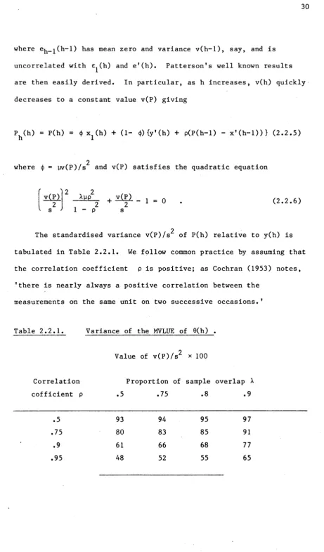
The standardised variance v(P)/s of P(h) relative to y(h) is

tabulated in Table 2.2.1. We follow common practice by assuming that

the correlation coefficient p is positive; as Cochran (1953) notes,

'there is nearly always a positive correlation between the

measurements on the same unit on two successive o c c a s i o n s . '

Table 2.2.1. Variance of the MVLUE of 9(h) .

Value of v(P)/s^ * 100

Correlation Proportion of sample overlap X

cofficient p .5 .75 .8 .9

93 94 95 97

80 83 85 91

61 66 68 77

48 52 55 65

.5

.75

.9

The general pattern of results is well known. For a fixed value

of p , v(P) is minimised by matching half of the sample units

(X = 0.5) , although the variance is fairly insensitive to the value of X until it is close to 1. For weakly correlated observations

(p < 0.6) , the gains from minimum variance estimation are considered to be quite modest.

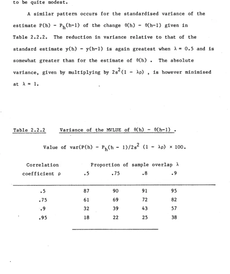
A similar pattern occurs for the standardised variance of the estimate P(h) - P^(h-l) of the change 9(h) - 9(h— 1) given in

Table 2.2.2. The reduction in variance relative to that of the

standard estimate y(h) - y(h-l) is again greatest when X = 0.5 and is

somewhat greater than for the estimate of 9(h) . The absolute

2

variance, given by multiplying by 2s (1 - Xp) , is however minimised at X = 1.

Table 2.2.2 Variance of the MVLUE of 6(h) - 9(h-l) .

Value of var(P(h) _{- ph<h -} l)/2s2 (1 - Xp) x 100

Correlation Proportion of sample overlap X

coefficient p .5 .75 .8 .9

.5 87 90 91 95

.75 61 69 72 82

I n p r a c t i c e , t h e v a l u e of p w i l l ne ed t o be e s t i m a t e d f ro m t h e d a t a and w i l l d i f f e r from i t e m t o i t e m . Ho we v er , some c ompr omis e v a l u e ca n be c h o s e n , o f t e n w i t h l i t t l e l o s s i n e f f i c i e n c y , a t l e a s t f o r t h e i t e m s of g r e a t e s t i n t e r e s t . F o r w e a k l y c o r r e l a t e d d a t a , t h e g a i n s f ro m MVLUE a r e m od es t and t h e s t a n d a r d e s t i m a t e y ( h ) g i v e n by p = 0 , <j> = y w i l l be u s e d . F o r h i g h l y c o r r e l a t e d i t e m s , p c a n be

r e p l a c e d by 1.

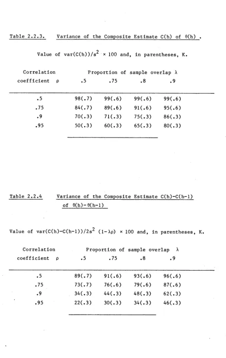
A s l i g h t l y m o d i f i e d f or m o f t h i s e s t i m a t o r w i t h p = 1 i s u s e d i n t h e C u r r e n t P o p u l a t i o n S u r v e y t a k e n m o n t h l y by t h e US B u r e a u of t h e C e n s u s . The c o m p o s i t e e s t i m a t o r u s e d i n t h i s s u r v e y t a k e s t h e f or m

C ( h ) = Ky(h) + ( 1 —K) { y ' ( h ) + C ( h - l ) - x ’ ( h - l ) } , ( 2 . 2 . 7 )

t h e t o t a l s a mp l e e s t i m a t e y ( h ) b e i n g u s e d r a t h e r t h a n x ^ ( h ) b a s e d o n l y on t h e newly s e l e c t e d u n i t s . Rao and Graham ( 1 9 6 4 ) g i v e f o r m u l a e f o r t h e v a r i a n c e o f C( h) and C( h) - C ( h - l ) u n d e r t h e

c o r r e l a t i o n a s s u m p t i o n s of ( 2 . 2 . 1 ) and comput e t h e v a r i a n c e o f t h e s e e s t i m a t e s r e l a t i v e t o t h a t of y ( h ) and y ( h ) - y ( h - l ) r e s p e c t i v e l y w i t h optimum v a l u e s of K.

T a b l e 2 . 2 . 3 and T a b l e 2 . 2 . 4 g i v e c o r r e s p o n d i n g r e s u l t s f o r t h e r o t a t i o n d e s i g n c o n s i d e r e d h e r e , t h e v a l u e s o f K u s e d b e i n g t h e same f o r b o t h C( h ) and C ( h ) - C ( h - l ) and a c ompr omi se b e t w e e n t h e i r

Table 2.2.3. Variance of the Composite Estimate C(h) of 9(h) . 2

Value of var(C(h))/s x 100 and, in parentheses, K.

Correlation Proportion of sample overlap X

coefficient p .5 .75 .8 .9

.5 98(.7) 99(.6) 99(.6) 99(.6)

.75 84(.7) 89(.6) 91 (* 6 ) 95(- 6)

.9 70(.3) 71(.3) 75(.3) 86(.3)

.95 50(.3) 60(.3) 65(.3) 80(.3)

Table 2.2.4 Variance of the Composite Estimate C(h)-C(h-1)

of 8(h)- 8(h-l)

Value of var(C(h)-C(h-l))/2s^ (1-Xp) x 100 and, in parentheses, K.

Correlation Proportion of sample overlap X

c o e f f i c i e n t p .5 . 7 5 .8 . 9

.5 8 9 ( . 7 ) 9 1 ( . 6 ) 9 3 ( . 6 ) 9 6 ( . 6 )

. 7 5 7 3 ( . 7 ) 7 6 ( . 6 ) 7 9 C . 6 ) 8 7 (. 6 )

.9 3 4 ( . 3 ) 4 4 ( . 3 ) 4 8 ( . 3 ) 6 2 ( . 3 )

2.3 BLU Estimation of 0(h) - Known Mean

In this section, the MSE of the BLUE of the population mean 0(h) derived using the unbiased estimates P(h), C(h) and y(h) are

compared. The mean of the process {0(t)} is assumed known and thus,

without loss of generality, set equal to zero. The results provide a

lower bound to the MSE of the BLUE under the more general assumption that the trend is a polynomial in the time element t with fixed coefficients.

Following Blight and Scott (1973), we assume that the process (0(t)} is first order autoregressive with

0(t) = a0(t-l) + v(t) (2.3.1)

where the (v(t)} are i.i.d. random variables with mean zero and 2

variance a . Written as a model for ( 0(t),©(t— 1)) (2.3.1)

v becomes

(2.3.2)

and in combination with the observation equation (2.2.3), the BLUE of ( 0(h),0(h— 1)) is given directly by the recursive updating equations of the Kalman filter. These are the results obtained by Blight and Scott (1973) using a Bayesian approach under normal distribution

assumptions. In particular, if 0 ( h ) is the BLUE of 0(h) , the MSE

B

of 0 ( h ) decreases to a limiting value, v ( 0 ) say, as h increases,

B B

where v ( 0 ) is given by the positive root of the quadratic equation B

8 ( t ) _a 0 e ( t - D v ( t )

= +

v(

V

v(

V

(1+R) -R - 0 (2.3.3)

and R = Var(8(t))/s2 = o^/(1 - a2 )s2

0 ( h ) is the fully efficient BLUE of 9(h) derived under the

B

model 0.(1) = 6 + e (1) (equations (1.4.1) to (1.4.5)), where

h h h

0^(1) is the MVLUE of using all the data available to time h and thus includes revised estimates for all previous occasions. A

simpler alternative in general is to use the unrevised estimate P(t), t = h, h-1,... .

In this case, Patterson (1950) shows that P(t) is a first order autoregressive process with parameter 8 = (1 - <J>) p (see (2.2.5)) and can thus be represented by a series of independent observation equations

P(t) - 8P(t-l) _{[1 -ß]}

9( t)

e( t - i )

+ Zp (t), t=2,... ,h

where the Z p (t) are i.i. d. random variables with mean zero and

variance < /'“

N

N

•n

II _{(1 - 02 ) v(P) .}

Let

_V

*)1 = (0p (h), 0p(h-l)) be the estimate of

( 6(h), 0(h-l)) at time h with MSE V (0 ) . The estimate and its MSE h P

are then given recursively by the Kalman updating equations

v h | h - i ( V

-~ a 0

1 0

a 1

0 0

+ 1 ! o q n > c o o 1 _ _ _ _ _ _ _ 1

^ ( h | h - l ) =

~ a 0"

1 0

% W Vh l h - l ( ^ ) "

1

1 - B

v ( z p )-1(P(h)-BP(h-l))

The MS E v^ (0p ) of 0p(h) r e duces to a con stant v(0 p) as h incr ea ses ,

and e q u a t i n g v, (0_) = v _(0_) = v( 0 ) in the e q u a t i o n

h P h-1 P P

V V

IWl

-1

+ 1

j

Vi(V v(V

*— v

give s

v( 0p)

v(P)

(or 3)' (l-a2 )(l-B2 )

v(6p )

v(P)

Var( 6( t))

1 v(P)

Var( 9(t) ) _ v (P )

P u t t i n g Rp = Var( 0 ( t ) ) / v ( P ) , ^ = 1/ ( 1 + R p ), Up = R p / ( 1 + R p ) = l“ Xp

and P a = ± ( a - 3)/(1 - aB) and rearranging,

' v < ep )

. v(P)

V(9P )

1-p2 v(p)

a

0 (2.3.4)

w h i c h is e x actly the form of e q u a t i o n (2.2.6), the e q u a t i o n for the

v a r i a n c e v(P) of the M V L U E P(h).

T he BLUE b ased on C(h) and y(h) can not be d e rived in this s imple

recu r s i v e manner. F o r the p u r p o s e of c o m p u t i n g thei r MSE, we use the

s ignal e x t r a c t i o n forms d e v e l o p e d by Scot t and Smith (1974) and

With y(t) = 9(t) + e(t) ,the BLUE ©^(h) of 6(h) given the series y(t): t=l,...,h is given by

0 (h) = y(h) - -iy Z

o j=0 k=0 E

\

n(h-j)

where I a y(t-k) = n(t) is the autoregressive representation of k k

y(t) , the (n(t)} are i.i.d. random variables with mean zero and 2

variance a , and c^(e) = cov(e(t),e(t-k)). The MSE of Qy(h) , denoted v ( 0^) is

V ( 0 Y ) = s2 - \ Z

o j=0 k=0 Z \ ci+k(e)J

(2.3.5)

The BLUE 0(h) of 9(h) given C(t): t=l,...,h and its MSE v ( 0 ) are derived in the same way.

The values c,(e) appropriate to 0 (h) are given by equation

k. Y

(2.2.2). From (2.2.7), C(h) can be written

C(h) = (l-K)C(h-l) + Ky(h) + (1-K)(y,(h) - x ’(h-l))

(l-K)C(h-l) + z (h) c

where, under the assumption (2.2.1), the covariances c . (z ) = cov(z (h), z (h-j)) are

J C C c

cQ(zc) = {k2 + 2K(l-K)(l-p) + 2(1-K)2(1-p)/a} s2

c (zc) = {K2 (l-jy)pj + K(l-K) 1~ (jx+1-)- (l-p)p3

- K(l-K) (1 -1 H) H/ (l-p)p3 1 - (1-K)2 1 (j+ 1 ^ (1-p)2 pj 1 } s2 A

Cj(zc) = 0 for j > g - 1. Given K,X, p and s , c^(zc) is computed from the above and var(C(h)) = v(C) from the formula given by Rao and

Graham (1964, p. 498, equation (15)). The covariances

Cj(C) = cov(C(t),C(t-j)) are given recursively by

2( 1K)c1(C) = (1 + (1K)2 ) v(C)

-(l-K)Cj(C) = (1 + (1-K)2 ) 0

<

_

j

. ₁

i—

• o '—✓

c ,(C) = (1-K)c 0 (C) + c (

g"l g-2 g-1

c. (C )

J

= (l-K)c. .(C)

J-l , j>g-l

0 c'

These are the covariances used in place of Cj(e) i-n (2*3.5) for

computing v ( 9 ) .

2

Given these sample covariances and the parameters a and of

model (2.3.1), the autocovariance pattern of the unbiased estimator

is obtained as the sum C_. ( 9) + Cj(e ) where C^(9) = oPo2 /(l-a2 ) • The

appropriate autoregressive moving average model (ARMA) is then fitted using the methods described by Box and Jenkins (1970, p. 498,

Program 2) and values of the autoregressive coefficient a^ 2

and o obtained. v ( 9^) and v ( 9^) can then be evaluated.

Note that in computing these values, the form of the model to fit to the autocovariance pattern is known exactly from our

assumptions. In practice the model would only be estimated, adding

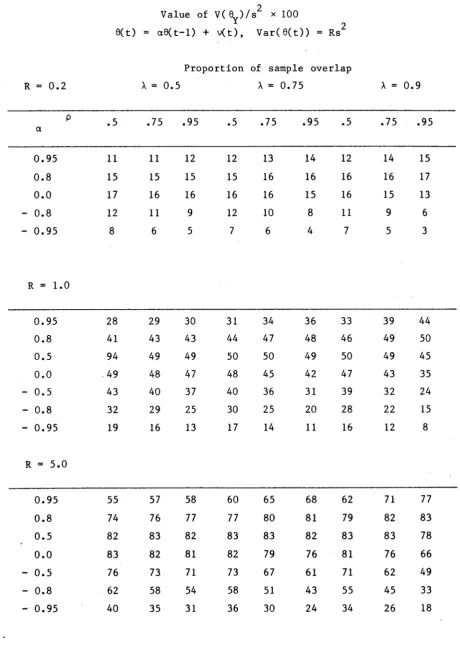
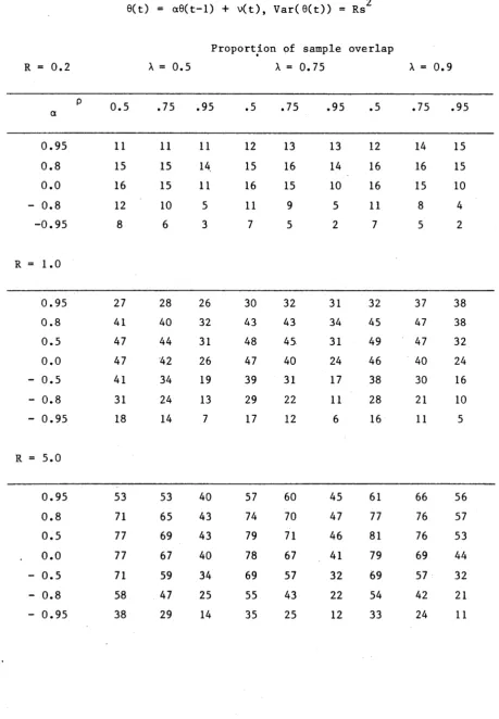
T a b l e 2 . 3 . 1 and T a b l e 2 . 3 . 2 g i v e v a l u e s f o r t h e MSE of t h e BLUE f o r n o n - o v e r l a p p i n g s u r v e y s ( A=0) and p a n e l s u r v e y s ( A=l)

r e s p e c t i v e l y . I n e i t h e r c a s e , MVLU e s t i m a t i o n p r o c e d u r e s o f f e r no i m p r o v e m e n t o v e r t h e s t a n d a r d s i n g l e s u r v e y e s t i m a t e y ( h ) and t h u s a l l t h e BLUE a r e e q u a l t o 0^(10 • E q u a t i o n ( 2 . 3 . 4 ) w i t h Rp = R t h e n

2

a p p l i e s t o v ( 0^) so t h a t , i n p a r t i c u l a r , v ( 9 Y) ( l + R ) / s R < 1 , i s a minimum when A^ = = 1/2 and h e n c e when R = 1, a n d , as a f u n c t i o n o f R, i s s y m m e t r i c a b o u t R = 1. F u r t h e r , u n l e s s | p | i s r e a s o n a b l y

2

l a r g e , v( 0y) ( 1 + R ) /s R i s n o t s u b s t a n t i a l l y l e s s t h a n 1.

F o r n o n - o v e r l a p p i n g s u r v e y s , 3=0 an d p = ± a . Thus v ( 9 )

a y

O

a t t a i n s i t s maximum v a l u e s R / ( 1+R) w i t h R f i x e d when a = 0 and

a d d i t i o n a l r e d u c t i o n s i n MSE a r e m o d e s t u n l e s s | a| i s l a r g e . C l e a r l y i f R i s s m a l l , t h e g a i n s f rom BLU e s t i m a t i o n a r e s u b s t a n t i a l .

Table 2.3.1 MSE of the BLUE of 0(h) - Non-overlapping Su r v e y s .

2

Value of v( Q ^ / s x 100

9(t) = a9(t-l) + v(t), Var(9(t)) = R s 2

For R < 1, v(9y (R)) = Rv^ C r” 1)) .

a R = 1 R = 5 R = 1C

± 0.95 24 48 60

± 0.8 38 69 80

± 0.5 46 80 89

0.0 50 83 91

Table 2.3.2 MSE of the BLUE of 0(h) - Panel Surveys

2

Value of v(9y )/s x 100

0(t) = a9( t - 1) + v(t), Var( 9( t ) ) = R s 2

For R < 1, v ( 0y (R )) = Rv(9y(R- 1 )) .

R = 1 R = 5 R = 10

P

.5 .75 .95 .5 .75 .95 .5 .75 .95

a

0.95 34 42 50 64 75 83 76 85 91

0.8 46 50 44 80 83 77 89 91 87

0.5 50 48 34 83 81 64 91 90 76

0.0 46 40 24 80 72 48 89 83 60

-Q.5 38 29 15 69 57 33 80 70 43

-0.8 27 20 9 53 41 21 66 53 28

o

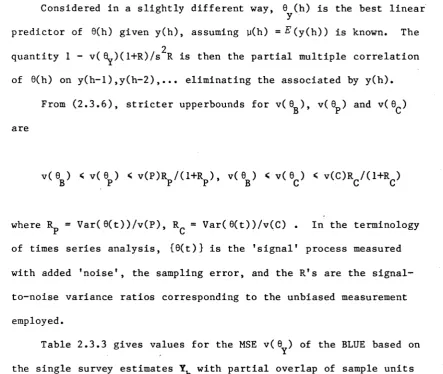
The q u a n t i t y s R / ( l + R ) i s an u p p e r bound t o t h e MSE of t h e BLUE of 6( h) i r r e s p e c t i v e of t h e c o r r e l a t i o n p a t t e r n s o f t h e s a mp l e

o b s e r v a t i o n s and p o p u l a t i o n p a r a m e t e r mod e l ( w i t h known me a n ) . From t h e r e s u l t s of C h a p t e r 1 w i t h we h a v e by a v e r s i o n of t h e C a u c h y - S c h wa r z i n e q u a l i t y ( Ra o, 1973, p 60)

MS E ( t r Q ) = i TK £ - 1TK Var(Y, ) 1 K £

h e e h e

T 2

„ ( I K X)

T e

£ K £ - s u p — — ---X X V a r ( Y , ) X

h T 2 T ( l K e l ) <

---£ V a r ( Y , ) ---£

h ( 2 . 3 . 6 )

w i t h e q u a l i t y i f and o n l y i f £ « V a r ( Y ^ ) £ .

T T 2

F o r t h e e s t i m a t e of 6 ( h ) , £ = ( 1 , 0 , . . . , 0 ) and £ K^£ = s g i v i n g t h e r e s u l t , w i t h t h e u p p e r b o u n d b e i n g a t t a i n e d w h e n e v e r

C o v ( 9 ( h ) , O ( h - j ) ) = R c o v ( e ( h ) , e ( h - j ) ) f o r a l l j .

F u r t h e r , t h e BLUE of 0( h) t h e n r e d u c e s t o

0 ( h) = y ( h ) - ( y ( h ) - y ( h ) ) / ( l + R )

y