https://doi.org/10.1007/s11242-018-1036-z
Modelling pH-Dependent and Microstructure-Dependent
Streaming Potential Coefficient and Zeta Potential of
Porous Sandstones
P. W. J. Glover1
Received: 30 November 2017 / Accepted: 7 March 2018 / Published online: 17 May 2018 © The Author(s) 2018
Abstract In this paper, we have significantly modified an existing model for calculating the
zeta potential and streaming potential coefficient of porous media and tested it with a large, recently published, high-quality experimental dataset. The newly modified model does not require the imposition of a zeta potential offset but derives its high salinity zeta potential behaviour from Stern plane saturation considerations. The newly modified model has been implemented as a function of temperature, salinity, pH, and rock microstructure both for facies-specific aggregations of the new data and for individual samples. Since the experi-mental data include measurements on samples of both detrital and authigenic overgrowth sandstones, it was possible to model and test the effect of widely varying microstructural properties while keeping lithology constant. The results show that the theoretical model rep-resents the experimental data very well when applied to model data for a particular lithofacies over the whole salinity, from 10−5to 6.3 mol/dm3, and extremely well when modelling indi-vidual samples and taking indiindi-vidual sample microstructure into account. The new model reproduces and explains the extreme sensitivity of zeta and streaming potential coefficient to pore fluid pH. The low salinity control of streaming potential coefficient by rock microstruc-ture is described well by the modified model. The model also behaves at high salinities, showing that the constant zeta potential observed at high salinities arises from the develop-ment of a maximum charge density in the diffuse layer as it is compressed to the thickness of one hydrated metal ion.
Keywords Microstructure·Porosity·Streaming potential·Zeta potential·Electrical rock
properties
B
P. W. J. Glover [email protected]List of Symbols
Cf Pore fluid salinity (mol/dm3)
Csp Streaming potential (coupling) coefficient with respect to pressure (mV/MPa)
F Formation factor,F φ−m(–)
K1 Equilibrium constant for solution of CO2in water.pK1−log10K1(–)
K2 Equilibrium constant for solution of CO2in water.pK2−log10K2(–)
K(−) Disassociation constant for dehydrogenization of silanol surface sites. pK(−) −log10K(−)(–)
Kme Binding constant for cation adsorption.pKme−log10Kme(–)
Kw Disassociation constant of water.pKw−log10Kw(–)
N Avogadro’s number, ~ 6.022×10+23/mol (mol−1)
pHexpt pH at which the experiments were run (arithmetic mean value) (–)
pHst.dev Standard deviation inpHexpt(–)
T Temperature (°C or K)
a 1. Fitting parameter in Eq. (1) for zeta potential (mV). 2. Constant in the Theta Transformation,8/3 for clastic rocks (–)
b Fitting parameter in Eq. (1) for zeta potential (mV)
dgr Modal grain diameter (m)
e Elementary charge, ~ 1.602×10⁻¹⁹C (C)
k Boltzmann’s constant, ~ 1.3806×10⁻²³J/K (J/K)
m Cementation exponent (–) βNa+ Na+Ionic fluid mobility (m2/s/V) βH+ H+Ionic fluid mobility (m2/s/V) βCl− Cl−Ionic fluid mobility (m2/s/V) βOH− OH−Ionic fluid mobility (m2/s/V) βStern Stern layer mobility
εr Relative dielectric permittivity of the pore fluid (–)
εo Absolute dielectric permittivity of a vacuum, ~ 8.854×10⁻¹²F/m (F/m) ζ Zeta potential (mV)
ηf Pore fluid viscosity (Pa s) σs Measured surface conductivity (–) φ Total porosity (–)
χζ Shear plane distance (m) Γo
s Density of mineral surface sites for complexation (sites/nm2) Λ Characteristic length scale of the pores (m)
Prot
s Protonic surface conductance/specific conductivity (S) s Total surface conductance/specific conductivity (S)
1 Introduction
its inclusion allowed the model to work well. However, at the time of its inclusion it had no satisfactory formal interpretation.
Consequently, an experimental campaign was initiated to produce a large database of 1253 measurements ofCspandζof the highest possible quality, using pore fluids which were fully equilibrated with the rock samples, where pore fluid salinity, conductivity and pH were all accurately measured, which were supported by a full suite of associated petrophysical mea-surements made on individual samples, and where the dataset contains a large number (324) of measurements with a salinityCf> 1 mol/dm3(Walker and Glover2017). The availability of this dataset offers the opportunity to carry out a detailed modelling campaign.
This paper reports that modelling campaign, and is, we believe, the most comprehensive modelling ofCspandζ carried out so far. The first aim of the work described in this paper was to modify the existingCspandζtheoretical model (Glover and Déry2010; Glover et al.
2012,2015) in order to fully representpHvariation in electrolytes. In previous models, the
pHwas allowed to vary as a function of temperature and with the addition of acids and bases but not as a function of salinity. The second aim was to replace the unjustified zeta potential offset with a modelling approach that takes into account the development of a maximum charge density in the diffuse layer as it is compressed to the thickness of one hydrated metal ion in thickness at high salinities. The third aim was to attempt to model the data of Walker and Glover (2017) both by facies and for individual rock samples and, in so doing, confirm (1) the operation of the low salinity control of microstructure onCsp, (2) examine the role of pH variations onCspandζ, and (3) investigate the possible physical causes of the zeta potential offset hypothesized by Jaafar et al. (2009) and Vinogradov et al. (2010).
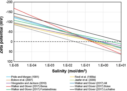
There have been several attempts to model theζ andCsp of rocks. Pride and Morgan (1991) produced an empirical fit to 35 existingζ data as a function of salinity in the low salinity range,Cf< 0.1 mol/dm3. They obtained
ζ a + blog10(Cf) , (1)
whereζis in volts andCfis in mol/dm3,a+ 8 mV andb+26 mV. Although this relationship describes the main aspects of the data to which it was fitted well, it provides positiveζ at salinities > 0.5 mol/dm3, whereas the physical model of the mineral/fluid interface would predict a negative value trending towards zero, and all measurements that have been made so far at high salinities provide extremely small but negative values (Jaafar et al.2009; Vinogradov et al.2010; Walker et al.2014, Walker and Glover2017). Similar empirical fits have been carried out by a number of authors with similar results: Walker and Glover (2017) provideda+ 3.505±28.823 mV andb+ 11.33±4.06 mV and for their entire dataset as well as carrying out fits to individual facies, Vinogradov et al. (2010) obtaineda+ 9.67 mV andb+ 19.02 mV, Jaafar et al. (2009), which share some data with Vinogradov et al. (2010), suggesteda+6.43 mV andb+ 20.85 mV. Bolève et al. (2007) suggesteda+ 14.6 mV andb+ 29.1 mV, while Revil et al. (1999a) have estimated the values ata≈+ 10 mV andb
≈+ 20 mV. However, these fits are simply empirical relationships. Their similarity (as shown in Fig.1) underlines a general trend. However, all of these fits produce positiveζ at high salinities, whereas none of the 400 or so measurements forCf> 1 mol/dm3so far are positive (Jaafar et al.2009; Vinogradov et al.2010; Walker and Glover2017); they all have small constant negative values instead. Clearly the empirical approach is limited, and a physically based theoretical model is required.
Fig. 1Representation of 10 existing empirical fits ofζas a function of pore fluid salinity showing approxi-mately the same behaviour but with unexplained high salinity behaviour and variability with pH
their more general equations, which were (1) that pH7, (2) that the fluid is an Na+or K+ symmetric electrolyte, (3) that the influence of H+and OH−ions on the ionic strength of the solution saturating the pores can be neglected (Revil and Glover1997), and (4) that direct adsorption of K+and Na+ions upon the silica surface can also be neglected.
Under these conditions
a 2kT
3e ln
√
8000εrεokT N
2eΓo s K(−)
10−pH
, (2)
and
b kT
3e loge10, (3)
wherek is Boltzmann’s constant (~ 1.3806×10⁻²³J/K),T is the temperature (in K),eis the elementary charge (~ 1.602×10⁻¹⁹ C),εris the relative dielectric permittivity of the pore fluid,o is the absolute dielectric permittivity of a vacuum (~ 8.854×10⁻¹²F/m),N is Avogadro’s number (~ 6.022×10+23/mol),Γso is the density of surface sites, andK(−)is the disassociation constant for dehydrogenization of silanol surface sites. The gradient of ζ versus log10(Cf) then depends only on temperature withb=+19.38 mV whenT= 20 °C, while the offset at the same temperature isa +16.89 mV for reasonable choices of its input parameters (pH≡7,Γo
s 10 sites/nm2,K(−)10−8, and assumingεr 80), which are discussed later in this paper. This model gives values ofζ which remain negative for the entire salinity range, tending towards zero at high salinities (Cf≈7.4 mol/dm3, which is just higher than the saturation limit for NaCl in water atCsat≈6.16 mol/dm3) as required by the physical model.
[image:4.439.93.350.55.239.2]result would not take into account the properties of the rock such as porosity, grain size and cementation exponent. In 2010, Glover and Déry (2010) provided the equations required to calculate theCspof individual rocks, taking into account their individual microstructural properties. That paper, which considered packs of glass beads, implemented a full theoretical description ofζ (Revil et al.1999a), andCspwas then calculated for the grain size, porosity and cementation exponent of the glass bead packs. The modelling was capable of representing the sigmoidally shaped variation of streaming potential with grain size (Glover and Déry
2010), but was restricted to the ideal matrix geometry imposed by the bead packs.
The theory was developed further and published in a form which could be applied to porous granular media (Glover et al.2012) and was validated against a database of 290
Cspand 269ζ measurements made by a large number of researchers. Unfortunately this database did not contain sufficient information about the salinity, electrical conductivity and pH of the fluids in contact with the grains of the rock at the time that the streaming potential measurement was made. In many cases, the experimental temperature was not measured or reported and information about the microstructural properties of the samples that were being measured was not measured or given. Although this dataset represented all the data that were available, it was not considered a stringent test of the theoretical model. Consequently, new experimental approaches (Walker et al.2014) were developed to make a large number of well-constrained measurements for testing the model, which are reported in full in Walker and Glover (2017) and form the experimental base with which the modelling in this paper is compared.
2 Reference Data
A full description of the reference data can be found in Walker and Glover (2017). This modelling uses the entire dataset of 1253Cspmeasurements and their derivedζ, representing 14 samples of 4 sandstone facies (Berea, Boise, Lochaline and Fontainebleau sandstones). Several separate examples of Fontainebleau and Lochaline sandstones composed of sub-rounded detrital grains, and consisting of detrital grains with euhedral quartz overgrowths, were measured (distinguished by the additional letter ‘D’ and ‘Q’ in the sample codes, respectively). A brief summary of sample properties measured during initial characterisation is shown in Table1of Walker and Glover (2017). The quality of the experimental data is generally good, having been measured at pore fluid equilibrium and with well-defined salinity and pH. However, the early data from one of the Berea sandstone (BR1) and one of the Boise sandstone samples (B1II) are less good and this is due to immature experimental protocols, as described in Walker and Glover (2017).
3 Electro-kinetic Modelling
It should be noted that modelling has been carried out at the temperature at which the individual data were measured, but instead of implementing one modelling curve for the experimental pH, a range of different models with different pHs have been implemented and shown as 5 modelling curves which divide the zeta potential–pore fluid salinity space and streaming potential–pore fluid salinity space. This approach has the advantage of informing the reader how the model behaves with both changes in pore fluid salinity and pH in one plot. The experimental data are then added to the plot following a trend which lies on or is parallel to a curve for one of the modelled pHs. Conformity of the model to the experimental data can then be judged by comparing the experimentally derived pH (provided in the data tables) with that indicated by how the experimental data fall on the network of modelled curves for different pHs. Despite there being many variables in the model, only one,K(−), was varied to improve the conformity of the model curves to the experimental data, and then only over a very restricted range supported by independent measurements for this parameter (please see Sect.3.7).
3.1 Modelling Procedure
The modelling has the following steps:
1. Define the temperature, fluid salinity range and fluid pH over which the modelling is to take place.
2. Calculate the density of pure water in kg/m3 at the modelling temperatureT in (°C) using
ρw 1000 1−(T+288.9414)
508929.2×(T+68.12963)(T−3.9863)
2. (4)
3. Calculate the density of the NaCl solution (in g/cm3) at the given salinity (in mol/dm3) and temperature using
ρf 58.44Cf+ ρw 1000
1000 − 58.44Cf 2.16
. (5)
4. Calculate the molality of the NaCl solution (in mol/kg) at the given salinities (in mol/dm3) and temperature using
cf
Cf
ρf − 58.44Cf
1000. (6)
5. Calculate the pore fluid electric permittivity using Olhoeft’s empirical equation (Revil et al.,1999b)
εf εoεr εo ao + a1T + a2T2 + a3T3 + c1Cf + c2Cf2 + c3Cf3
, (7)
whereao295.68,a1−1.2283/K,a2−2.094×10−3/K2,a3−1.41×10−6/K3,
c1−13.00 dm3/mol,c2−1.065 (dm3/mol)2,c3−0.03006 (dm3/mol)3, the tem-perature is in Kelvin and is valid in the range 273–373 K, the salinity is in mol/dm3and the permittivityin vacuoo8.854×10−12F/m (Lide2017).
6. Calculate the pore fluid electrical conductivityσfusing Sen and Goode’s method (Sen and Goode1992a,b).
8. Calculate the ionic concentration of the pore fluid including contributions from acids and bases that are added to perturb the pH to give the pH to be modelled. This step uses the imposed salinity with the addition of the concentrations of hydrogen and/or base ions to arrive at the desired pH value. It is not sufficient to calculate these from the desired pH and pOH because the pore fluid is also in equilibrium with atmospheric carbon dioxide. Consequently, the pH depends on the concentrations of hydrogen and base ions according to a cubic law. We solve the cubic law automatically in our model using Cardano’s method (Glover et al.2012). This approach also requires knowledge of the disassociation constant for waterKw, for which an empirical equation is available in Lide (2017) and described in full in Glover et al. (2012).
9. Calculate theζof the sample (Glover et al.2012). 10. Calculate theCspof the sample (Glover et al.2012).
The model outputs for this work areCspandζ. The calculation ofCsprequires three addi-tional parameters, which are all microstructural parameters that are specific to the individual rock sample. Theζis calculated for a given mineralogy, fluid type (electrolyte type, salinity and pH) and temperature and is usually considered to be independent of the microstructure of the individual rock, while it is clear from experiments thatCspdepends upon the microstruc-ture of the individual rock, at least at low salinities (Glover et al.2015; Walker and Glover
2017).
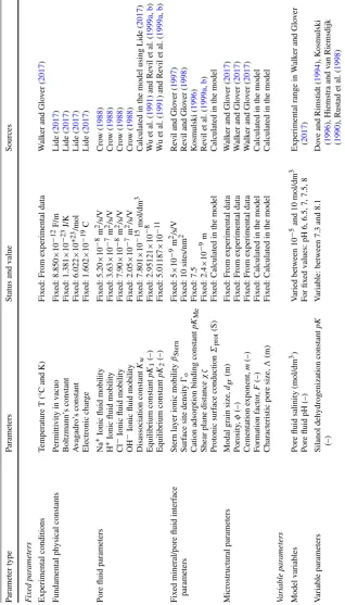
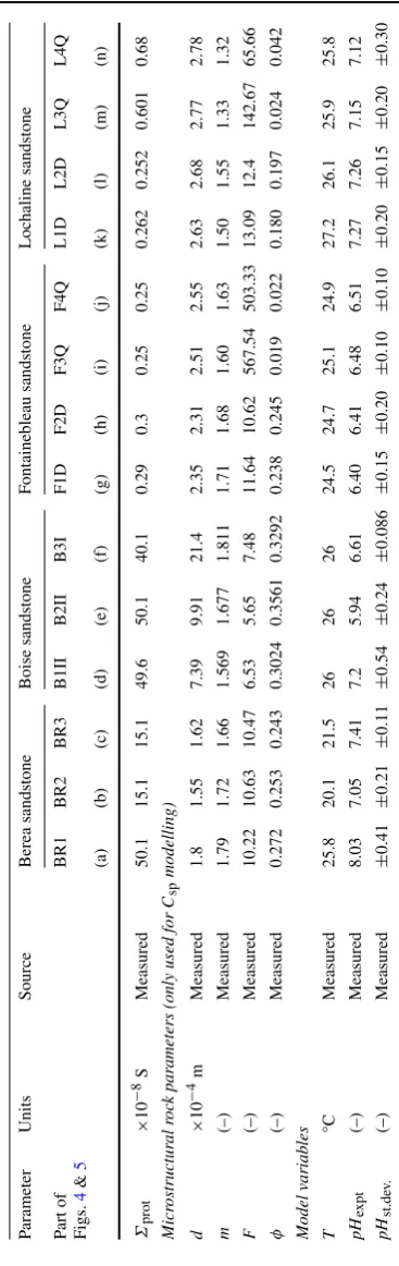
All parameters are discussed below, separating them into groups. The parameters used in this paper for the modelling by rock type and for individual samples can be found in Tables2
and3, respectively, together with a note of their sources. It should be noted that while many parameters contribute to the model, almost all are fixed either by independent experimental measurements made in this paper or by other researchers or perform as modelling variables.
3.2 Modelling Variables
There are three parameters which are modelling variables. These are temperature, salinity and pH. In this work, the salinity and pH have been varied between 10−5and 10 mol/dm3, and between pH 5.5 and pH 8.5, respectively. The salinity is used to calculate the concentration of ions in the solution together with the concentration of H3O+and OH−, which are calculated from the fluid pH. The model is not strongly sensitive to temperature. Nevertheless, the temperature for each modelling run has been fixed to the mean experimental temperature given in Walker and Glover (2017).
3.3 Pore Fluid Parameters
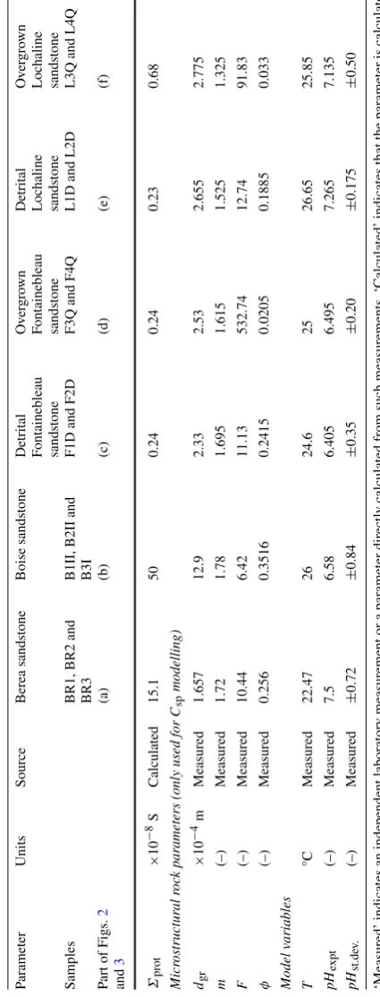
Ta b le 2 The m ean v alues of parameters u sed in the modelling o f the ζ and Csp for each rock type together with their source P arameter Units Source Berea sandstone Boise sandstone
Detrital Fontainebleau sandstone
Ov er gro w n F ontainebleau sandstone Detrital Lochaline sandstone
Ov er gro w n Lochaline sandstone Samples BR1, BR2 and BR3 B1II, B2II and B3I F1D and F2D F 3Q and F 4Q L1D and L2D L 3Q and L 4Q P art of Figs. 2 and 3 (a) (b) (c) (d) (e) (f) Fluid par ameter s Fluid type NaCl NaCl NaCl NaCl NaCl NaCl βNa+ × 10 − 8m 2/s/V Cro w ( 1988 ) 5 .20 5 .20 5 .20 5 .20 5 .20 5 .20 βH+ × 10 − 8m 2/s/V Cro w ( 1988 ) 36.3 36.3 36.3 36.3 36.3 36.3 βCl– × 10 − 8m 2/s/V Cro w ( 1988 ) 7 .90 7 .90 7 .90 7 .90 7 .90 7 .90 βOH– × 10 − 8m 2/s/V Cro w ( 1988 ) 20.5 20.5 20.5 20.5 20.5 20.5 pK 1 (–) R ev il and G lo v er ( 1998 ) 7.53 7.53 7.53 7.53 7.53 7.53 pK 2 (–) R ev il and G lo v er ( 1998 ) 10.3 10.3 10.3 10.3 10.3 10.3 Interface par ameter s βStern × 10 − 9m 2/s/V Re vil and Glo v er ( 1997 ) 555555 Γ o s Sites/nm 2 Re vil and Glo v er ( 1998 ) 10 10 10 10 10 10 pK me (–) K
osmulski (1996
Ta b le 2 continued P arameter Units Source Berea sandstone Boise sandstone
Detrital Fontainebleau sandstone
Ov er gro w n F ontainebleau sandstone Detrital Lochaline sandstone
[image:10.439.57.270.62.619.2]3.4 Mineral/Fluid Interface Parameters
There are six parameters which describe the mineral/fluid interface. Of these, the ionic mobil-ity in the Stern layer βStern, the surface site density Γo, the binding constant for cation adsorptionpKMe, and the shear plane distanceχζhave all been held constant throughout this work (Table1). Each, however could be adjusted within the limits imposed by the indepen-dent experimental measurements that are noted in Walker et al. (2014) and discussed fully in Glover et al. (2012). The Stern layer mobility has been taken asβStern 5×10⁻⁹m2/s/V from Revil and Glover (1997), the surface site density has been taken asΓo10 sites/nm2 from Revil and Glover (1998) and the binding constant for cation adsorption has been taken aspKMe7.5 from Kosmulski (1996). The shear plane distance (χζ). The model is sensitive to this parameter because it defines where in the diffuse layer theζis measured. In this work, it was held constant atχζ2.4×10⁻⁹m for all the samples.
The fifth interface parameter is the specific surface conduction. In this paper we use it to provide a measurement of the protonic surface conduction (prot) for each of the rock samples. The specific surface conduction was calculated from the measured surface conduc-tivityσsusing the modal grain diameterdgr, and the cementation exponentmand formation factorFfor each sample. The surface conductivity was taken to be the conductivity that was measured when the rock was saturated with the lowest salinity equilibrium fluid. These surface conductivities were converted to surface conductancessusing the relationship
σs 2ΣsΛ, (8)
where is a characteristic length scale for the pores of the rock that was introduced by Johnson et al. (1986) and which can be calculated with the equation (Revil and Cathles1999)
Λ dgr
2m F. (9)
Consequently, Eqs. (8) and (9) provide individual values of surface conductancesfor each sample. There are three contributions to surface conduction, arising from (1) the move-ment of protons on the surface, (2) ionic mobility in the Stern plane, and (3) ionic mobility in the diffuse layer. We have assumed that the value of surface conductance calculated using Eqs. (8) and (9) above is the same as the protonic surface conduction. This assumption has been justified by using the model to calculate and compare the three contributions to surface conduction as a function of salinity and pH. In all cases the calculated contributions to surface conduction from the diffuse layer and Stern layer were more than two orders of magnitude less than the calculated total surface conductance at all values of pH and salinity. Hence, it was possible to say that the remaining contribution, that of the protonic surface conduction, makes up the great majority of the surface conduction, and thatprot≈s. Consequently, for the purposes of this paper,protis completely defined by independent measurements ofσs,
dgr,mandF. The surface conductivity can also be obtained empirically from the formation factor measured at ultra-low salinities and the pore fluid conductivity, as implemented by Lorne et al.1999a,b) and others, but this approach is more suited to experimental research rather than modelling.
The last interface parameter is the disassociation constant for dehydrogenization of silanol
pK(−). It has been taken to vary in the restricted range 8.1 >pK(−)> 7.3, which fall in the middle of the range of values given by other researchers:pK(−)6.8 (Dove and Rimstidt
1994),pK(−)6.5 (Kosmulski1996),pK(−)7.5 (Hiemstra and van Riemsdijk1990), and
only parameter which has been varied in this way since the modified model does not now contain a zeta potential offset parameter as described below.
3.5 The Zeta Potential Offset
In earlier modelling (Glover and Déry2010; Glover et al.2012; Glover et al.2015) there was an additional mineral/fluid interface parameter called the zeta potential offset (ζo). In this work, the zeta potential offset has been replaced by a procedure which holdsζconstant at high salinities, which models the attainment of a maximum charge density in the diffuse layer as it is compressed to the thickness of one hydrated metal ion in thickness according to the hypothesis of Jaafar et al. (2009). This modelling procedure recognises the onset of such behaviour and keeps theζ constant at salinities higher than this onset value. The values of constantζobtained using this approach vary with pH, as noted in the experimental measurements of Walker and Glover (2017) and produce values which are in the same range (−8 to−20 mV) as those obtained in earlier modelling (Glover and Déry2010; Glover et al.
2012,2015).
The previous method was essentially the addition of an ‘ad hoc’ parameter that allowed the model to work at high salinities while retaining its precision at low and medium salinities. The addition was not carried out with regard to any underlying physics and could be viewed as a parameter that could be varied to ensure a better fit of the model to the data. However, values of zeta potential offset found in this way had a very restricted range, indicating that they were the result of some unknown physical process (Glover and Déry2010; Glover et al.
2012). The new method accepts the hypothesis of Jaafar et al. (2009) and has the advantages of (1) removing the only arbitrary parameter from the model, (2) reducing the number of variables in the model (to one in this work), and (3) having the modified model based more soundly on our understanding of the physical process occurring in the porous rocks.
3.6 Rock Microstructural Parameters
Finally, there are five parameters which describe the microstructure of the rock sample. Only three of them, however, are independent. The parameters are the modal grain sizedgr, porosity φ, cementation exponentm(Glover and Déry2010), formation factorF, and characteristic pore size. They are inter-related by Eq. (9) and Archie’s first law (e.g., Glover et al.2015)
F φ−m. (10)
It is worth noting that it is also possible to express the theoretical model in terms of pore sizedp(Glover and Walker2009) and pore throat sizedpt(Glover and Déry2010) using the relationships
dp dgr
8φ2m
am2 , (11)
dpt ≈ dp
1.665, (12)
respectively. In this work, we have opted to use grain size, porosity and cementation exponents as the three independent parameters to describe the microstructure of each rock sample.
the modal grain size by laser diffractometry. The microstructural parameters that were used in the modelling are shown in tables later in the paper.
3.7 Degrees of Freedom
Consequently, the model has a number of different types of parameter as summarised in Table1. There are 3 model variables, which are parameters to whichCspandζ are known to be sensitive and which have been varied to explore these relationships, 4 fundamental physical quantities, 12 pore fluid and interface parameters which are defined by external measurements and held constant during the modelling, 5 microstructural parameters that are defined by petrophysical measurements that have been carried out on the samples and consequently also held constant during the modelling. There is only one parameter, the disassociation constant for the dehydrogenisation of silanolpK(−), which has been varied to
improve the fit of the model to the experimental data, and then only within the very restricted range (8.1 >pK(−) > 7.3) which has been fixed by independent measurements from other authors. Consequently, the degree to which the model curves presented in this work fit the experimental data is not a consequence of varying a large number of parameters until some sort of fit is attained, but the result of varying one parameter over a small range and having all the other parameters fixed by independent measurements on the particular samples or other parameters measured by independent researchers.
4 Theoretical Modelling Results
Since we know the microstructural (porosity, cementation exponent and modal grain size) and the experimental fluid parameters (equilibrated salinity, electrical conductivity andpH) for each sample, we have been able to carry out modelling of individual samples as well as for aggregated lithofacies.
In this section the figures and discussion of theζ modelling are followed by those related to theCsp, which is the order in which they are calculated in the theoretical model. Despite this order, it should be remembered that for the experimental results, it is theCspthat is derived first, directly from streaming potential and pressure difference measurements, while theζis derived subsequently from theCspusing additional parameters.
4.1 Modelling by Lithofacies
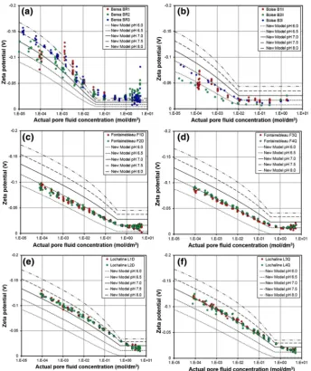
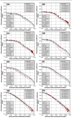
Figures2and3show, respectively, all of theζandCspmodelling curves we have calculated for each of the six lithofacies (Berea, Boise, and detrital and overgrowth forms of both Fontainebleau and Lochaline sandstones) from this paper compared with all of the data for these lithofacies from Walker and Glover (2017). The modelled curves extend for the complete relevant salinity range (10−5–10 mol/dm3) and frompH6 topH8 in increments of half apH unit. In each case the curves are calculated for the temperature at which the experimental measurements were taken. The lithofacies modelling was carried out with mean values of the microstructural parameters for each lithofacies and which are shown in Table2. Figure2shows the calculatedζ model curves as a function of salinity and pH together with the data from Walker and Glover (2017) and arranged by lithofacies. The model curves use mean microstructural parameters for the samples composing each lithofacies.
Fig. 2Modelledζ (curves) for all facies types as a function of pore fluid salinity andpH, compared with the experimental measurements ofζ (symbols) from this paper.aBerea sandstone,bBoise sandstone,c
detrital Fontainebleau sandstone,dovergrown Fontainebleau sandstone,edetrital Lochaline sandstone, and
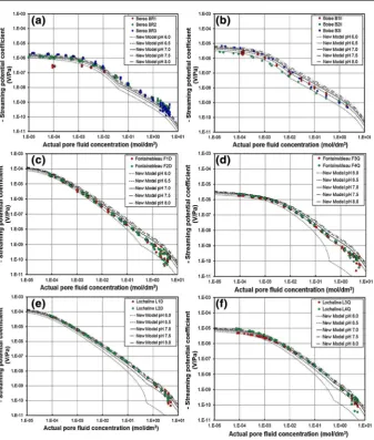
[image:14.439.48.393.52.463.2]Fig. 3ModelledCsp(curves) for all facies types as a function of pore fluid salinity andpH, compared with the experimental measurements ofCsp(symbols) from this paper.aBerea sandstone,bBoise sandstone,
cdetrital Fontainebleau sandstone,dovergrown Fontainebleau sandstone,edetrital Lochaline sandstone, andf overgrown Lochaline sandstone. All model parameters are shown in Table2. In this model, there are 19 independent parameters, of which 3 are model variables (temperature, fluid salinity andpH), 13 are predefined by the electro-chemistry of the fluid and fluid-mineral interface, and 3 are predefined by the rock microstructure (dgr,m,φ). The model retains only 1 variable parameter (pK(−)), which was allowed to vary in the experimentally restricted range 8.0 >pK(–) > 7.5
[image:15.439.53.391.46.444.2]measurements are difficult to make (Vinogradov et al.2010; Walker et al.2014; Walker and Glover2017). However, the modelζcurves agree well with the mean of this cloud of points. Figure3shows the calculatedCspmodel curves as a function of pore fluid salinity and
pHtogether with the data from Walker and Glover (2017) and arranged by lithofacies. Once again, it is clear that theCspmodel curves reproduce all of the main features of the experimentally measured data, with the value ofCspincreasing in an approximately power law fashion as pore fluid salinity is reduced. TheCspmodel curves are also sensitive to pore fluid pH, but not to the same degree as theζcurves, and this is also noted in the experimental data. It was hypothesised by Glover et al. (2012) that the flattening ofCspat low salinities, which is clear in experimental data (e.g., Walker and Glover2017) is controlled by the development of surface conduction and the microstructure of the rocks on the basis of a comparison of their model with the experimental data then available. Comparison of the modelling carried out in this paper with the new data in Walker and Glover (2017) has confirmed the effect. OurCspmodelling for each of the two microstructural forms of Lochaline and Fontainebleau sandstone (i.e., between parts (c) and (d) and parts (e) and (f) in Fig.3) shows that varia-tions in their independently measured microstructural parameters (modal grain size, porosity, cementation exponent and/or formation factor) and surface conduction (in the absence of any mineralogical differences) are sufficient to explain the degree of flattening occurring in the experimentalCspdata. In each case the quartz overgrown version shows a greater degree of low salinity flattening, and this is well-modelled by smaller porosities and cementation exponents which occur for these samples (the measured grain sizes and values of surface conduction are not significantly different).
It should be noted that there is no microstructural control on zeta potential because it is a property of the electrical double layer (EDL) which occurs between the mineral grain and the pore fluid and can be regarded as a property acting on a grain surface scale, independent of how those grains are arranged in a microstructure. This is discussed in more detail at the end of Sect.4.2.
4.2 Sample-by-Sample Modelling
The model has been implemented for each sample measured by Walker and Glover (2017) for a range of salinities andpHat the experimental temperature and with the microstructural and electrical parameters (modal grain size, porosity, cementation exponent, and formation factor) that were measured for that sample.
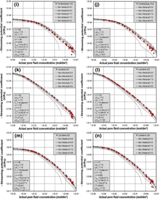
As in the case of the modelling by lithofacies, the electro-chemical parameters that describe the interface between the rock matrix and the pore fluid could be adjusted to ensure a best fit. However, once again, only one was varied (pK(−)). The full sample parameters and the modelling parameters are shown in Table3. Figures4and5show the sample-specificζand
Cspcurves from the theoretical model as well as the relevant experimental data from that sample, forCf ranging from 10−5 to 10 mol/dm3 and for five values ofpH in the range 6 <pH< 8. ThepH of the pore fluid was controlled and measured during the experiments of Walker and Glover (2017) to within±0.2, which is given aspHexptin the data tables in this paper. This value should be used to interpret how the values of the experimental data in Figs.4and5compare with the set of modelledζ andCspcurves for the five values ofpH for which modelling has been implemented.
Ta b le 3 The p arameters u sed in the modelling o f the Csp and ζ for indi vidual samples (Figs. 4 and 5 ) P arameter Units Source Berea sandstone Boise sandstone F ontainebleau sandstone Lochaline sandstone Pa rt o f Figs. 4 & 5 BR1 BR2 BR3 B1II B2II B3I F 1D F2D F 3Q F4Q L 1D L2D L 3Q L4Q (a) (b) (c) (d) (e) (f) (g) (h) (i) (j) (k) (l) (m) (n) Fluid par ameter s Fluid type NaCl NaCl NaCl NaCl NaCl NaCl NaCl NaCl NaCl NaCl NaCl NaCl NaCl NaCl βNa+ × 10 − 8m 2/s/V Cro w ( 1988 ) 5 .20 5 .20 5 .20 5 .20 5 .20 5 .20 5 .20 5 .20 5 .20 5 .20 5 .20 5 .20 5 .20 5 .20 βH+ × 10 − 8m 2/s/V Cro w ( 1988 ) 36.3 36.3 36.3 36.3 36.3 36.3 36.3 36.3 36.3 36.3 3 6.3 3 6.3 3 6.3 3 6.3 βCl– × 10 − 8m 2/s/V Cro w ( 1988 ) 7 .90 7 .90 7 .90 7 .90 7 .90 7 .90 7 .90 7 .90 7 .90 7 .90 7 .90 7 .90 7 .90 7 .90 βOH– × 10 − 8m 2/s/V Cro w ( 1988 ) 20.5 20.5 20.5 20.5 20.5 20.5 20.5 20.5 20.5 20.5 2 0.5 2 0.5 2 0.5 2 0.5 pK 1 (–) R ev il and G love r ( 1998 ) 7.53 7.53 7.53 7.53 7.53 7.53 7.53 7.53 7.53 7.53 7.53 7.53 7.53 7.53 pK 2 (–) R ev il and G love r ( 1998 ) 10.3 10.3 10.3 10.3 10.3 10.3 10.3 10.3 10.3 10.3 10.3 10.3 10.3 10.3 Interface par ameter s βStern × 10 − 9m 2/s/V Re vil and G love r ( 1997 ) 5.00 5.00 5.00 5.00 5.00 5.00 5.00 5.00 5.00 5.00 5.00 5.00 5.00 5.00 Γ o s Sites/nm 2 Re vil and G love r ( 1998 ) 10 10 10 10 10 10 10 10 10 10 10 10 10 10 pK me (–) K
osmulski (1996
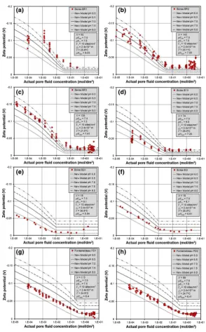
Fig. 4Modelledζ(curves) for individual samples as a function of pore fluid salinity andpH, compared with the experimental measurements ofζ(symbols) from this paper.aBerea (BR1),bBerea (BR2),cBerea (BR3),
[image:19.439.72.367.49.523.2]Fig. 4continued
the Fontainebleau and Lochaline sandstone samples. For example, the data for the sample of detrital Fontainebleau sandstones F1D and F2D, shown in Fig.4g, h, fall clearly on the curve for apH= 6.5 in each diagram. The experimentally measuredpH for these measure-ments waspHexp= 6.40 and 6.41. The data for the Berea and Boise sandstones have a greater scatter, however, even here the mean behaviour agrees very well with the theoretical curves. For example, the Berea sandstone sample BR3 hasζ andCspdata that follow a trend the mean behaviour of which would lie on a theoretical curve for pH 7.5, while the measured pH during the experiment was pHexp 7.41.
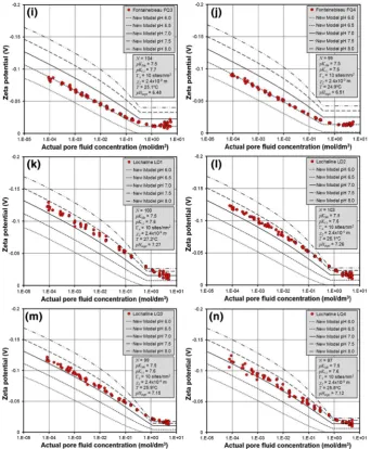
[image:20.439.49.392.54.469.2]Fig. 5ModelledCsp(curves) as a function of pore fluid salinity andpH, compared with the experimental measurements ofCsp(symbols).aBerea (BR1),bBerea (BR2),cBerea (BR3),dBoise (B1II),eBoise (B2II),
fBoise (B3I)gFontainebleau (F1D),hFontainebleau (F2D),iFontainebleau (F3Q),jFontainebleau (F4Q),
[image:21.439.73.367.46.533.2]Fig. 5continued
experimental data is also is modelled well by replacing the ad hocζoffset that was used in previous models with our new approach, which keeps theζ at a constant level for salinities above which the thickness of the diffuse layer is approximately the same or less than the diameter of a hydrated metal ion.
[image:22.439.54.386.56.470.2]line, while for Lochaline sandstones, Fig.4k-n shows the experimentally determinedζ fall between the modelled curves forpH7 andpH7.5.
We have calculated coefficients of determination for the comparison of theζdata for each sample and the theoretical curve calculated for the pH at which the measurements were made (pHexpt) and find that the coefficient of determination (R2) values are in all cases > 0.89. Hence the experimental observation thatpHis one of the major controls on theζ, and that even small changes in pH (e.g.,pH7±1) can lead to a large change inζ(Walker and Glover,
2017) is now supported by modelling.
Considering theCspmodelling, Fig.5shows the modelledCspcurves as a function of salinity andpH for individual samples, taking into account their individual petrophysical properties. TheCspmodel curves reproduce all of the main features of theCspdata extremely well. The overall approximate power law behaviour is overlain with a flattening at low salinities and curvature at moderate salinities for some values ofpH, both of which conform to the experimental data. In general, the use of sample-specific parameters improves the agreement between the theoretical model curves and the experimental data compared to the modelling in Fig.3, and the agreement between the theory and the experimental data is in many cases excellent.
Disagreement occurs for specific salinities where there may be systematic errors in the experimental data (e.g., for 10−4 mol/dm3for Berea sandstone BR1, Fig.5a), and there is an overestimation of the theoretical model at low salinities for the Boise sandstone samples (i.e., for B1II, B2II and B3I, Fig.5d–f), which probably arises from using inappropriate modelling parameters. The agreement could be improved if we had taken the approach of fitting the theoretical model to the experimental data, but the goal of this work was not to fit the theoretical model to the data but to see how robust the theoretical model is when compared to high-quality data. The agreements between theory and experiment in the sample-by-sample study represented by Figs.3and5are better than any published so far.
TheCspmodel curves are sensitive to pore fluid pH just as in Fig.3, but now it is possible to see clearly that the experimental data fall close to the theoretical curve for the experimental value ofpH(pHexpt), which is given for reference on each plot and in Table3, together with the uncertainty in its measurement. A typical example is for Berea sample BR3 (Fig.5c), where the experimental data fall almost exactly on the curve forpH 7.5 and for which the mean experimentalpHwas 7.41±0.11 (Table3). We have calculated coefficients of determination for the comparison of theCspdata for each sample and the theoretical curve calculated for thepHat which the measurements were made (pHexpt), and find that theR2values are in all cases > 0.91.
the pores are connected, leaving the cementation exponent relatively unchanged. After the overgrowths are developed, electrically patent pathways still occur along thin passageways between the euhedral grains, but their sensitivity to closure, which is measured by the large formation factor, is high. The increase in formation factor is primarily due to the significant reduction in porosity than a change in cementation exponent. There is little change in grain size because the overgrowths are filling-in pore space rather than increasing the size of the grain in all directions. This is akin to comparing the diameter of a sphere with a co-centred cube of the same linear dimensions—the cube has a volume that is almost twice as big (6/π 1.9099), yet seems to occupy a similar amount of space.
Once again, it should be noted that there is no microstructural control on zeta potential. The zeta potential is a property of the electrical double layer (EDL) which occurs between the mineral grain and the pore fluid. It is calculated from the Stern potential which itself is obtained by assuming that the EDL is thin compared to its extent (Fixman1980,1983). Consequently, it can be regarded as a property acting on a grain surface scale and should be independent of how those grains are arranged in a microstructure. That will certainly be the case when the EDL is extremely small at high pore fluid salinities. However, there is a possibility that the zeta potential might vary in a rock at a local scale when the pore fluid salinity is so low that the EDL is of the same scale as the characteristic scale of the pores. In this case, the shear plane might vary from location to location within the microstructure as fluid flow conforms to that microstructure. This will give rise to local, transient potential dif-ferences which can be regarded as microstreaming potentials. However, the electro-neutrality requirement will ensure that most of these microstreaming potentials cancel each other out so that we are left with the macroscopic overall streaming potential. A similar effect can also be imagined to arise from a rock composed of a mixture of minerals with different Stern potentials and consequently different zeta potentials. Consequently, the effect will have an influence on how the zeta potential from two different minerals in a two-mineral mixture mix to provide an effective zeta potential.
5 Conclusions
A modified form of the theoretical model of Glover et al. (2012) has been applied to all of the data from Walker and Glover (2017) for each lithofacies and for each individual sample. The major modifications to the model comprised (1) implementing a calculation for pore fluid pH that is a function of all the ionic contributions to the electrolyte, (2) removing the zeta potential offset as a parameter forcing a constantζat high salinities, (3) implementing a variable thresholdζ at high salinities where the thickness of the diffuse layer is comparable to the size of the hydrated metal ions and representing, therefore, a maximum charge density for the diffuse layer. The modelling was carried out as a function of salinity and pH allowing only one parameter (the disassociation constant for dehydrogenation of silanol) to vary over a small range constrained by independent measurements made by other researchers.
The modelledζ curves were found to agree well with the experimental data for each lithofacies and extremely well for each individual sample. The modelledζis highly sensitive to pH and salinity, and it was found that the experimental data fell on the curves expected from the experimental pH, in most cases to within±0.2pHpoints, contrasting with the widespread scatter of previously existingζ measurements which suffered a lack ofpHcontrol.
the low salinity behaviour of theCspmeasurements is caused by the pore structure and best exemplified by the difference results obtained when measuring either the detrital or overgrown forms of the Fontainebleau and Lochaline data, each of which is chemically indistinguishable. The replacement of the zeta potential offset with an implementation of the maximum charge density hypothesis of Vinogradov et al. (2010) for generating a constant value of ζ at high salinities (to match the experimental observations) has led to a modelling which concords extremely well with all of the data in the Walker and Glover (2017) dataset.
It should be noted that this paper concerns itself only with sandstones. The model it describes does not take into the account the complex mineralogy of rocks that comprise clays, which affect the mineral–electrolyte interfacial chemistry. In order to make the model applicable to a wider range of rocks, a proper surface complexation model (e.g., Datta et al.,
2009; Li et al.,2016) should be incorporated in order to yield the equilibrium zeta potential of each type of mineral before calculating the effective zeta potential value for each rock sample and then calculating the streaming potential from the individual rock sample microstructural parameters. The surface complexation models, when validated against experimental data, could provide a route for evaluating the zeta potential under varying concentration, compo-sition and temperature.
Acknowledgements The funding for this work was provided by the Natural Sciences and Engineering Research Council of Canada (NSERC) Discovery Grant Programme and a start-up grant from the University of Leeds. I am indebted to two anonymous reviewers who substantially contributed to the quality of this paper.
Open Access This article is distributed under the terms of the Creative Commons Attribution 4.0 Interna-tional License (http://creativecommons.org/licenses/by/4.0/), which permits unrestricted use, distribution, and reproduction in any medium, provided you give appropriate credit to the original author(s) and the source, provide a link to the Creative Commons license, and indicate if changes were made.
References
Bolève, A., Crespy, A., Revil, A., Janod, F., Mattiuzzo, J.L.: Streaming potentials of granular media: influence of the Dukhin and Reynolds numbers. J. Geophys. Res.112, B08204 (2007).https://doi.org/10.1029/ 2006JB004673
Crow, D.R.: Principles and Applications of Electrochemistry. Chapman and Hall, London (1988)
Datta, S., Conlisk, A.T., Li, H.F., Yoda, M.: Effect of divalent ions on electroosmotic flow in microchannels. Mech. Res. Commun.36(1), 65–74 (2009)
Dove, P.M., Rimstidt, J.D.: Silica–water interactions. Rev. Mineral. Geochem.29, 259–308 (1994) Fixman, M.: Charged macromolecules in external fields. I. The sphere. J. Chem. Phys.72(9), 5177–5186
(1980)
Fixman, M.: Thin double layer approximation for electrophoresis and dielectric response. J. Chem. Phys.
78(3), 1483–1491 (1983)
Glover, P.W.J.: Electrical Properties, 2nd ed. Treatise Geophys, vol. 189. Elsevier, London (2015)
Glover, P.W.J., Déry, N.: Dependence of streaming potential on grain diameter and pore radius for quartz glass beads. Geophysics75(6), F225–F241 (2010).https://doi.org/10.1190/1.3509465
Glover, P.W.J., Walker, E.: A grain size to effective pore size transformation derived from an electro-kinetic theory. Geophysics74(1), E17–E29 (2009)
Glover, P.W.J., Walker, E., Jackson, M.D.: Streaming-potential coefficient of reservoir rock, a theoretical model. Geophysics77(2), D17–D43 (2012).https://doi.org/10.1190/GEO2011-0364.1
Hiemstra, T., Van Riemsdijk, W.H.: Multiple activated complex dissolution of metal (hydr)oxide: a thermo-dynamic approach applied to quartz. J. Colloid Interface Sci.136, 132–150 (1990).https://doi.org/10. 1016/0021-9797(90)90084-2
Johnson, D.L., Koplik, J., Schwartz, L.M.: New pore-size parameter characterizing transport in porous media. Phys. Rev. Lett.57(20), 2564–2567 (1986).https://doi.org/10.1103/PhysRevLett.57.2564
Kosmulski, M.: Adsorption of cadmium on alumina and silica: analysis of the values of stability constants of surface complexes calculated for different parameters of triple layer model. Colloids Surf. A117, 201–214 (1996).https://doi.org/10.1016/0927-7757(96)03706-5
Li, S., Leroy, P., Heberling, F., Devau, N., Jougnot, D., Chiaberge, C.: Influence of surface conductivity on the apparent zeta potential of calcite. J. Colloid Interface Sci.468, 262–275 (2016)
Lide, D.R.: Handbook of Chemistry and Physics, 98th edn. Taylor Francis, London (2017). ISBN 1439880492 Phillips, S.L., Ozbek, H., Otto, R.J.: Basic energy properties of electrolytic solutions database: sixth Interna-tional CODATA Conference Santa Flavia (Palermo), Sicily, Italy, May 22–25, accessed 10 June 2010. https://www.osti.gov/bridge/purl.cover.jsp;jsessionid=3954E775156A8BC0FA35DB5CE5B402D4? purl=/6269880-iPJPhB/(1978)
Lorne, B., Perrier, F., Avouac, J.: Streaming potential measurements: 1. Properties of the electrical double layer from crushed rock samples. J. Geophys. Res: Solid Earth104(B8), 17857–17877 (1999a) Lorne, B., Perrier, F., Avouac, J.: Streaming potential measurements: 2. Relationship between electrical and
hydraulic flow patterns from rock samples during deformation. J. Geophys. Res.: Solid Earth104(B8), 17879–17896 (1999b)
Pride, S.: Governing equations for the coupled electromagnetics and acoustics of porous media. Phys. Rev. B
50(21), 15678–15696 (1994)
Pride, S.R., Morgan, F.D.: Electrokinetic dissipation induced by seismic waves. Geophysics56, 914–925 (1991).https://doi.org/10.1190/1.1443125
Revil, A., Cathles, L.M.: Permeability of shaly sands. Water Resour. Res.35, 651–662 (1999)
Revil, A., Glover, P.W.J.: Theory of ionic surface electrical conduction in porous media. Phys. Rev. B55, 1757–1773 (1997).https://doi.org/10.1103/PhysRevB.55.1757
Revil, A., Glover, P.W.J.: Nature of surface electrical conductivity in natural sands, sandstones, and clays. Geophys. Res. Lett.25, 691–694 (1998).https://doi.org/10.1029/98GL00296
Revil, A., Pezard, P.A., Glover, P.W.J.: Streaming potential in porous media. I. Theory of the zeta-potential. J. Geophys. Res.104(B9), 20021–20031 (1999a).https://doi.org/10.1029/1999JB900089
Revil, A., Schwaeger, H., Cathless, L.M., Manhardt, P.D.: Streaming potential in porous media 2. Theory and application to geothermal systems. J. Geophys. Res.104, 20033–20048 (1999b).https://doi.org/10.1029/ 1999JB900090
Rustad, J.R., Wasserman, E., Felmy, A.R., Wilke, C.: Molecular dynamics study of proton binding to silica surfaces. J. Colloid Interface Sci.198, 119–129 (1998).https://doi.org/10.1006/jcis.1997.5195 Sen, P., Goode, P.: Influence of temperature on electrical conductivity on shaly sands. Geophysics57, 89–96
(1992a)
Sen, P., Goode, P.: Errata, to: influence of temperature on electrical conductivity of shaly sands. Geophysics
57, 1658 (1992b)
Vinogradov, J., Jaafar, M.Z., Jackson, M.D.: Measurement of streaming potential coupling coefficient in sandstones saturated with natural and artificial brines at high salinity. J. Geophys. Res.115, B12204 (2010).https://doi.org/10.1029/2010JB007593
Walker, E., Glover, P.W.J.: A transient method for measuring the DC streaming potential coefficient of porous and fractured rocks. Transp. Porous Media (2017).https://doi.org/10.1002/2013JB010579
Walker, E., Glover, P.W.J., Ruel, J.: A transient method for measuring the DC streaming potential coefficient of porous and fractured rocks. J. Geophys. Res. (2014).https://doi.org/10.1002/2013JB010579 Wu, L., Forsling, W., Schlindler, P.W.: Surface complexation of calcium minerals in aqueous solution. J.