https://doi.org/10.1214/17-EJP61
[email protected]
https://eprints.whiterose.ac.uk/
Reuse
This article is distributed under the terms of the Creative Commons Attribution (CC BY) licence. This licence
allows you to distribute, remix, tweak, and build upon the work, even commercially, as long as you credit the
authors for the original work. More information and the full terms of the licence here:
https://creativecommons.org/licenses/
Takedown
If you consider content in White Rose Research Online to be in breach of UK law, please notify us by
El e c t ro n ic
Jo f
P
r o
b a b il i t y
Electron. J. Probab.22(2017), no. 39, 1–36. ISSN:1083-6489 DOI:10.1214/17-EJP61
The Brownian net and selection in the spatial
Λ
-Fleming-Viot process
Alison Etheridge
*Nic Freeman
†Daniel Straulino
‡Abstract
We obtain the Brownian net of [24] as the scaling limit of the paths traced out by a system of continuous (one-dimensional) space and time branching and coalescing random walks. This demonstrates a certain universality of the net, which we have not seen explored elsewhere. The walks themselves arise in a natural way as the ances-tral lineages relating individuals in a sample from a biological population evolving according to the spatial Lambda-Fleming-Viot process. Our scaling reveals the effect, in dimension one, of spatial structure on the spread of a selectively advantageous gene through such a population.
Keywords:Brownian net; spatialΛ-Fleming-Viot; branching; coalescing.
AMS MSC 2010:60G99; 60K35.
Submitted to EJP on November 23, 2016, final version accepted on April 23, 2017. SupersedesarXiv:1506.01158.
1 Introduction
The Brownian net, introduced in [24], arises as the scaling limit of a system of branching and coalescing random walk paths. It extends, in a natural way, theBrownian web, which originated in the work of [1]. In the Brownian web there is no branching. It can be thought of as the diffusive limit of a system of one-dimensional coalescing random walk paths, one started from each point of the space-time (diamond) lattice. Informally, the web is then a system of coalescing Brownian paths, one started from each space-time point. The Brownian web was formulated in [15] as a random variable taking its values in the space of compact sets of paths, equipped with a topology under which it is a Polish space. In this framework, the powerful techniques of weak convergence become available and as a result the Brownian web emerges as the limit of a wide variety of one-dimensional coalescing systems; e.g. [13], [20]. This points to a certain ‘universality’ of the Brownian web.
In the Brownian net, each path has a small probability (tending to zero in the scaling limit) of branching in each time step. The limiting object is (even) more difficult to
*University of Oxford, supported in part by EPSRC Grant EP/I01361X/1. E-mail:[email protected] †University of Sheffield. E-mail:[email protected]
to the Brownian net.
The original motivation for our work was a question of interest in population genetics: when will the action of natural selection on a gene in a spatially structured population cause a detectable trace in the patterns of genetic variation observed in the contemporary population? We deal with the most biologically interesting case of a population evolving in a two-dimensional spatial continuum in [6]. Our work in this paper uncovers some of the rich mathematical structure underlying mathematical models for biological populations evolving in one-dimensional spatial continua. In particular, we study the systems of interacting random walks that, as dual processes (corresponding to ancestral lineages of the model), describe the relationships, across both time and space, between individuals sampled from those populations.
It is natural to ask whether the model of [19] has a biological interpretation. It does: killing corresponds to a mutation term. This was observed by [24] (c.f. [7]). However, in view of the technical challenges to be overcome to handle the additional killing term, even on a diamond lattice, we do not explore this further here.
Our starting point will be the SpatialΛ-Fleming-Viot process with selection (SΛFVS) which (along with its dual) was introduced and constructed in [10]. The dynamics of both the SΛFVS and its dual are driven by a Poisson Point Process ofevents(which model reproduction in the population) and will be described in detail in Section 2. Roughly, each event prescribes a region in which reproduction takes place. A proportionυof the population in the affected region is replaced by offspring of a single parent. We shall refer toυ as the impact of the event. In the absence of selection, the dual process of ancestral lineages is a modification of the ‘Poisson trees’ of [13]. With selection, our dual follows ‘potential’ ancestral lineages, which introduces a branching mechanism, with the rate of branching determined by the presence of lineages in a region, but not increasing with their density. Our main result, Theorem 3.5, is that in one spatial dimension and when the impactυ= 1(which prevents ancestral lineages from jumping over one another), when suitably scaled the system of branching and coalescing ancestral lineages converges to the Brownian net.
Without selection, the corresponding objects converge (after scaling) to the Brownian web. In that setting, we believe (and [4] provides strong supporting evidence) that the random walks can even be allowed to jump over one another and the only effect on the limiting object is a simple scaling of time (given by one minus the crossing probability of ‘nearby’ paths). This would mirror the results of [20], in which systems of coalescing non-simple random walks with crossing paths are shown to converge to the Brownian web. When we try to include selection in this limit, allowing paths to cross has a more complicated effect, as we illustrate through simulations in Section 7. It is an intriguing open question to explain the pictures that we present there.
con-verges to branching Brownian motion, with coalescence of lineages at a rate determined by the local time that they spend together. In this article we are interested in a very different regime, in which coalescence of lineages is instantaneous on meeting.
Although our result owes a lot to the existing literature, the continuum setting introduces some new features. In particular, some care is needed in extending the self-duality of the systems of branching and coalescing simple random walks that appear in [24] to an ‘approximate’ self-duality of the càdlàg walks in continuous time and space that are considered here.
In Section 2 we introduce the SΛFVS and its dual before providing a heuristic explanation for our scaling. In Section 3 we provide a self-contained account of the necessary background on the Brownian web and net. Our main result is then stated formally in Theorem 3.5, which is proved in Sections 4-6. Finally, Section 7 presents a brief numerical exploration of the effect of allowing the random walk paths of the dual process to cross on the positions at time one of the left-most and right-most paths emanating from a point.
Acknowledgement
This work forms part of the DPhil thesis of the third author, [23]. We would like to thank the examiners, Christina Goldschmidt and Anton Wakolbinger for their careful reading of the result and their detailed feedback. We should also like to thank three anonymous referees for detailed and helpful comments. Just after we submitted the original version of this paper (and posted it on the arXiv), [22] appeared, providing a convenient set of criteria for convergence to the Brownian net. Following the suggestion of one of the referees, in this version we have adapted our proofs to exploit those criteria.
2 The S
Λ
FVS and its dual
In this section we introduce the set of branching and coalescing paths with which our main result is concerned. They arise as the dual to a special instance of the SΛFVS. The reader familiar with the SΛFVS can safely refer to Definition 2.2 (and the three lines preceding it) for notation, take note of Remark 2.3, and then skip to Section 3.
2.1 The SΛFVS
The Spatial Λ-Fleming-Viot process (SΛFV) without selection was introduced in [8, 2]. In fact the name does not refer to a single process, but rather to a framework for modelling the dynamics of frequencies of different genetic types found within a population that is evolving in a spatial continuum. It is distinguished from the classical models of population biology in that reproduction is based on ‘events’ rather than individuals. This introduces density dependence into reproduction in such a way that the clumping and extinction which plagues classical models is overcome, whilst the model remains analytically tractable. For a survey of the SΛFV we refer to [3].
There are very many different ways in which to introduce selection into the SΛFV. Here we adapt the approach typically adopted to introduce selection into the Moran model of classical population genetics. A full motivation of this approach can be found in [10], to which we refer the reader.
We suppose that the population is divided into two genetic types, which we denote
R× {a, A}with ‘spatial marginal’ Lebesgue measure, which we endow with the topology of vague convergence. By a slight abuse of notation, we also denote the state space of the process(wt)t∈RbyMλ.
Definition 2.1 (One-dimensional SΛFV with selection (SΛFVS)).Fix R ∈ (0,∞) and
υ∈(0,1]and letµbe a finite measure on(0,R]. Further, letΠbe a Poisson point process onR×R×(0,∞)with intensity measure
dx⊗dt⊗µ(dr). (2.1)
The one-dimensional spatial Λ-Fleming-Viot process with selection (SΛFVS) driven by(2.1)is theMλ-valued process(wt)t∈Rwith dynamics given as follows.
If (x, t, r) ∈ Π, a reproduction event occurs at time t within the closed interval
[x−r, x+r]. With probability1−sthe event(x, t, r)isneutral, in which case:
1. Choose a parental locationzuniformly at random within(x−r, x+r), and a parental type,κ, according towt−(z), that isκ=awith probabilitywt−(z)andκ=Awith
probability1−wt−(z).
2. For everyy∈[x−r, x+r], setwt(y) = (1−υ)wt−(y) +υ1{κ=a}.
With the complementary probabilitys,(x, t, r)corresponds to aselectiveevent within
[x−r, x+r]at timet, in which case:
1. Choose two distinct ‘potential’ parental locationsz, z′ independently and uniformly
at random within(x−r, x+r), and at each of these locations ‘potential’ parental typesκ,κ′, according tow
t−(z), wt−(z′)respectively.
2. For everyy ∈ [x−r, x+r] setwt(y) = (1−υ)wt−(y) +υ1{κ=κ′=a}. Declare the parental location to be z if κ = κ′ = a orκ = κ′ = A and to be z (resp. z′) if
κ=A, κ′ =a(resp. κ=a, κ′=A).
In fact this is a very special case of the SΛFVS introduced in [10], and even more special than those constructed in [9], but it already provides a rich class of models. We use the assumption thatµhas bounded support in Section 4, but it is far from necessary for the construction of the process. The assumption that parental locations are sampled uniformly from(−r, r)has become standard in the literature, but at no point do we use it; our proofs work equally well for any symmetric distribution on(−r, r). The parameter
2.2 The dual process of branching and coalescing lineages
Our primary concern in this paper is the dual process of the SΛFVS, a system of branching and coalescing paths that encodes all thepotential ancestorsof individuals in a sample from the population.
When there is no selection, the dual contains only coalescing random walks, and each such walk corresponds to the ancestral lineageℓof some individual; meaning thatℓ
traces out the locations in space-time occupied by the ancestors of that individual. If selection is present, then, at a selective event, we cannot determine the genetic types of the potential ancestors of the event (and hence the type and location of the actual ancestor) without looking further into the past. To avoid intractable non-Markovian dynamics, in this case we define a dual which traces all the locations in space-time which couldhave contained ancestors of a sampleSfrom the contemporary population. This leads to a system of branching and coalescing random walks, tracing all thepotential ancestral lineages.
The dynamics of the dual are driven by the same Poisson point process of events,Π, that drove the forwards in time process. The distribution of this Poisson point process is invariant under time reversal and so we shall abuse notation by reversing the direction of time when discussing the dual.
We suppose that at time0(which we think of as ‘the present’) we samplekindividuals from locationsx1, . . . , xk, and we writeξt1, . . . , ξtNt, for the locations of theNtpotential
ancestral lineages that make up our dual at timetbefore the present.
Definition 2.2(Branching and coalescing dual).FixR ∈(0,∞). LetΠbe a Poisson point process onR×R×(0,∞)with intensity measure
dx⊗dt⊗µ(dr)
whereµis a finite measure on(0,R]. The branching and coalescing dual process(Ξt)t≥0
is theSn≥1Rn-valued Markov process with dynamics defined as follows: At each event
(x, t, r)∈Π, with probability1−s, the event is neutral:
1. for each isuch thatξi
t− ∈ [x−r, x+r], mark the ithlineage with probabilityυ,
independently overiand of the past;
2. if at least one lineage is marked, all marked lineages disappear and are replaced by a single lineage (the ‘parent’ of the event), whose location at timetis drawn uniformly at random from within(x−r, x+r).
With the complementary probabilitys, the event is selective:
1. for each isuch thatξi
t− ∈ [x−r, x+r], mark the ithlineage with probabilityυ,
independently overiand of the past;
2. if at least one lineage is marked, all marked lineages disappear and are replaced bytwolineages (the ‘potential parents’ of the event), whose (almost surely distinct) locations are drawn independently and uniformly from within(x−r, x+r).
In both cases, if no lineage is marked, then nothing happens.
wt(x)is only defined at Lebesgue almost every pointxand so we have to be satisfied with a ‘weak’ moment duality.
Proposition 2.4 (Proposition 2.2 of [10]).The spatial Λ-Fleming-Viot process with selection is dual to the process (Ξt)t≥0 in the sense that for every k ∈ N and ψ ∈
C(Rk)∩L1(Rk), we have
Ew0
Z
Rk
ψ(x1, . . . , xk)
Yk
j=1
wt(xj)
dx1. . . dxk
= Z
Rk
ψ(x1, . . . , xk)E{x1,...,xk} YNt
j=1
w0 ξjt
dx1. . . dxk. (2.2)
In fact, a stronger form of this duality holds, in which the forwards in time process of allele frequencies and the process of potential ancestors of a sample are realised on the same probability space through a lookdown construction; see [25] for the case without selection and [9] for the general case.
From now on
forwards in time refers to forwards for the dual process, i.e. the reversal of that in Definition 2.1.
2.3 The scaling
We shall keep the impact of each reproduction event (i.e. the parameter υ) fixed, but we rescale the strengthsof selection. In addition we perform a diffusive rescaling of time and space. For our main result we requireυ = 1, but the heuristic argument presented here and the numerical experiments of Section 7, suggest that there should be a non-trivial limit for any fixedυ∈(0,1). Let us now describe the appropriate rescaling. The stages of our rescaling are indexed byn∈N.
Recall thatµis a finite measure on(0,R]. For eachn∈N, define the measureµnby µn(A) =µ(n1/2A),for all Borel subsets AofR. At thenth stage of the rescaling, our
rescaled dual is driven by the Poisson point processΠnonR×R×[0,∞)with intensity
n1/2dx⊗n dt⊗µn(dr). (2.3)
The√nin front ofdxarises since the rate at which centres of events fall in an interval of lengthlin the rescaled process is the rate at which they fall in an interval of length
√
nlin the unscaled process. Each event ofΠn, independently, is neutral with probability
1−snand selective with probabilitysn, wheresn =α/√nfor someα∈(0,∞). Thus, the
at a selective event. The two new lineages are born at a separation of order1/√n. If we are to ‘see’ both lineages in the limit then they must move apart to a separation of order1
(after which they might, possibly, coalesce back together). Ignoring possible interactions with other lineages, the probability that a pair of lineages achieves such a separation is of order1/√n. Therefore, in order to obtain a non-trivial limit (which differs from that in the absence of selection) we needO(√n)such branches per scaled unit of time, so we takensn=α√norsn=α/√n. (This argument can also be used to identify the correct scaling ofsnin order to obtain a non-trivial limit in higher dimensions, see [6].)
Evidently we can extend the duality of Proposition 2.4 to lineages that are sampled at different times. For each pointp= (x, t)∈R2, we think of an individual living at(x, t)
and, at thenth stage of the rescaling, construct the setP↑
n(p)of the potential ancestral lineages of the individual atp. (The reason for the uparrow in the notation will become clear in Section 4.1.) ThusPn↑(p)is a set of branching and coalescing paths. Our main result will concern the limit when we consider the union of such sets of paths aspranges over a countable dense set of space-time points.
3 The Brownian net
In order to state a precise result, we must introduce the Brownian net and, in particular, the state space in which convergence takes place. A short introduction to the Brownian web and net is provided in this section. For a detailed survey of the surrounding literature, see [22].
Once again, the reader familiar with this area can note our modification of the usual state space (detailed in Section 3.1) and Remark 3.1 for terminology, and then skip to the statement of our main result, which can be found in Section 3.3.
3.1 The state space
We now introduce the state space for our processes. Since our branching and coalescing paths are only càdlàg (not continuous), to capture the convergence ofPn↑(p) we will need a modification of the state space (introduced by [15]) that is commonly used for the Brownian web and net.
Fors∈[−∞,∞], we set
D[s] =f : [s,∞]→[−∞,∞] ;f is càdlàg on[s,∞]∩(−∞,∞) .
Forf ∈D[s], it will be convenient to defineσ(f) =σf =sto be the first time at whichf is defined. We set
M = [
t∈[−∞,∞]
D[t]. (3.1)
For each s ∈ [−∞,∞] andf ∈ D[s] we define a function f¯as follows. Let κt = tanh−1(t)and note thatκis an order preserving homeomorphism between[−1,1]and
[−∞,∞]. (The specific choice of the functiontanhis a convention in the literature. We use the symbolκin place oftanhto denote a change of time rather than rescaling of space.) Then iff ∈M we define
¯
f(t) =tanh(f(κt)) 1 +|κt|
(3.2)
fort∈[κ−1(σ
f),1]. It follows immediately thatf¯is càdlàg.
In Section 5.1 we define a generalizationρof the Skorohod metric that acts on càdlàg paths with possibly different starting times. We show (in Section 5.2) that
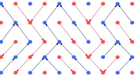
Figure 1: Self duality of systems of coalescing random walks on the diamond lattice that converge to the Brownian web. The blue arrows represent the forwards in time coalescing random walks, while the red arrows represent the backwards in time dual.
is a pseudo-metric onM. In standard fashion, from now on we implicitly work with equivalence classes ofM and, with mild abuse of notation, treat(M, dM)as a metric space. In view of (3.2), the intuition for (3.3) is that convergence in(M, dM)can be described as local Skorohod convergence of the paths plus convergence of the starting times.
If we restrict to continuous paths and replaceρwith the usualL∞ distance, then
we recover the space(M , df Mf)introduced by [15], see (5.21). Convergence in the corre-sponding metric on continuous paths can be described as locally uniform convergence of paths plus convergence of starting times.
We define the setK(M)of compact subsets ofM, equipped with the Hausdorff metric,
m, and including the empty set∅as an isolated point. We show (in Section 5.2) that
(M, dM)is complete and separable; the spaceK(M)inherits these properties. Similarly, we writeK(Mf)for the space of all compact subsets ofMf.
3.2 The Brownian web and net
Arratia [1] was the first to observe that the Brownian web exhibits a self-duality. It is most easily understood by first considering the prelimiting system of coalescing simple random walks, one started from each point of the diagonal space-time lattice. As illustrated in Figure 1, one can think of each path in the prelimiting system as the concatenation of a series of arrows, representing the jump made by the path out of each point ofZ at each timet ∈Z, and there is then a natural dual system of arrows (on the dual lattice), pointing in the opposite direction of time, which ‘fills out the gaps’ between the walkers forwards in time. It is not hard to convince oneself that the law of the resultant system of backwards paths is equal to that of the forwards system, rotated by180degrees about the origin(0,0). Under diffusive rescaling, the forwards and backwards systems converge jointly to a pair(W,Wc), known as the double Brownian web, in which W is the Brownian web and the dual webWchas the same law asW rotated by180degrees.
the SΛFVS; that is at thenth stage of the rescaling the probability that two paths, one stepping left and one stepping right, emanate from a given point isζ/√n.
In contrast to the Brownian web, the Brownian net will have a multitude of paths coming out of each space-time point. The key to its characterisation is that it has a well-defined left-most and right-most path, which we denotelz andrz respectively, emanating from each pointz= (x, t)∈R2and these determine what is called a left-right
Brownian web. Essentially, the set of left-most (resp. right-most) paths form a Brownian web with a leftwards (resp. rightwards) drift. Thus, for any deterministic pair of k -tuples of points(z1, . . . , zk),(z′1, . . . , zk′′), the left-most pathslz1, . . . , lzkare distributed as coalescing Brownian motions with driftζto the left, and the right-most pathsrz′
1, . . . rz′k′ are distributed as coalescing Brownian motions with driftζto the right.
Before we can fully describe the Brownian net, we must explain how a left-most path
lz =l(x,s) and a right-most pathrz′ =r(x′,s′) interact. Their joint evolution after time
s∨s′ is the unique weak solution to the left-right stochastic differential equation
dLt=ξ1{Lt6=Rt}dB l
t+ξ1{Lt=Rt}dB c t−ζdt, dRt=ξ1{Lt6=Rt}dB
r
t+ξ1{Lt=Rt}dB c t+ζdt,
(3.4)
where Bl
t, Btr andBtc are independent standard Brownian motions and if s < t then Ls≤Rs⇒Lt≤Rt. [24] proved (weak) existence and uniqueness of the solution to this system.
A straightforward extension of (3.4) is sufficient to specify the joint distribution of any finite collection of left-right paths, which are known as left-right coalescing Brownian motions.
Remark 3.1.In [24] the drift parameterζof the left-right stochastic differential equation used to construct the Brownian net is allowed to vary but the diffusion constant,ξ2, of
the Brownian motions is always taken to be one. Applying a linear time change to their construction yields generalξ2 and we will use such webs and nets (and results from
elsewhere extended trivially to apply to them) without further comment. We shall refer to the Brownian net corresponding to the left-right system (3.4) as the net with driftζ
and diffusion constantξ2.
It remains to give a rigorous characterization of the Brownian net. One last ingredient is required.
Definition 3.2.Letα: [σα,∞)→Randα′: [σα′,∞)→Rbe paths. We sayαcrossesα′ from left to right at timet∈Rif there existst−< tandt+> tsuch thatα(t−)
−α′(t−)<0
andα(t+)
−α′(t+)>0andt= inf
{s∈(t−, t+) ; (α(t−)
−α′(t−))(α(s)
−α′(s))<0 }. We define a crossing ofα′ byαfrom right to left analogously. We say thatαcrosses
α′ if it does so from either left to right or right to left.
Given two pathsαandα′which cross at say, timet, we can define a new pathgby
followingαup until timet, and subsequently followingα′. This procedure is known as
hoppingfromαtoα′ at the (crossing) timet. Given a setPof paths,H
cross(P)is defined to be the set of paths obtained by hopping a finite number of times between paths within
P.
Definition 3.3([24]).The Brownian netN is theK(Mf)valued random variable whose distribution is uniquely determined by the following properties:
1. For each deterministicz∈R2, almost surelyN contains a unique left-most pathlz
and a unique right-most pathrz.
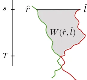
Figure 2:A wedge. In the notation of (3.5), the pathˆris inXˆr
n, and the pathˆlis inXˆnl. The last time at which both paths are defined iss, in this case given byσ(ˆl);rˆ(s)<ˆl(s)
and, tracing backwards in time,T is the first time at whichrˆ= ˆl. The wedge is the shaded region.
3. For any deterministic dense countable setsDl,Dr⊆R2,
N =Hcross({lz;z∈ Dl} ∪ {rz;z∈ Dr}).
The proof of our main result rests on verifying the conditions of Theorem 3.4, which provides criteria under which a sequence of processes converges to the Brownian net. It is obtained by combining Theorem 6.11 and Remark 6.12 of [22]. To state it, we require the notion of a wedge. Let( ˆXl
n)and( ˆXlr)be two random sets of paths such that their rotations by180degrees about(0,0)areK(Mf)valued random variables. Take
ˆ
l∈Xˆl
n andrˆ∈Xˆnr, defined on time intervals(−∞, σ(ˆl)]and(−∞, σ(ˆr)]respectively. We writes=σ(ˆl)∧σ(ˆr)for the largest time at which both paths are defined. Suppose that
ˆ
r(s)<ˆl(s)and defineT := sup{t < s: ˆr(t) = ˆl(t)}to be the first time time the paths meet (as we trace backwards in time). We call the open set
W(ˆr,ˆl) :={(x, u)∈R2:T < u < s,rˆ(u)< x <ˆl(u)} (3.5)
a wedge. This set is illustrated in Figure 2. We say that a pathπstarted at timeσπenters W from the outside if there existsσπ≤u < tsuch that(π(u), u)∈/ W and(π(t), t)∈W. Here,W denotes the closure ofW.
Theorem 3.4(Theorem 6.11, Remark 6.12 of [22]).Let(Xnl)and(Xnr)be two sequences
ofK(Mf)valued random variables. Let( ˆXl
n)and( ˆXlr)be two random sets of paths such
that their rotations by180degrees about(0,0)areK(Mf)valued random variables. Set
Xn=Hcross(Xnl ∪Xnr)andXˆn =Hcross( ˆXnl ∪Xˆnr).
Suppose that:
(A) Paths inXnl (resp.Xnr) do not cross. No path inXncrosses a path ofXnl from right to left, and no path inXn crosses a path ofXnrfrom left to right. No path inXnl
crosses a path ofXˆl
n, and no path ofXnr crosses a path ofXˆnr.
(B) For anyk∈N, and any(z1, . . . , z2k)⊆R×Rthere exists a convergent sequence
(ln,1, . . . , ln,k, rn,1, . . . ,n,k),
where ln,i ∈ Xnl, rn,i ∈ Xnr, whose limit (in distribution, inMf2k, asn → ∞) is a
(C) Wheneverk∈Nandlˆn∈Xˆnl andˆrn ∈Xˆnr are such that(ˆln,ˆrn)converges (inMf2,
in distribution, asn→ ∞) to left/right Brownian motions(ˆl,rˆ), the first meeting time ofˆlnwithrˆnalso converges in distribution to the first meeting time ofˆlwithrˆ.
(D) Paths ofXndo not enter wedges ofXˆnfrom the outside.
Then,Xnconverges (inK(Mf), in distribution) to the Brownian net.
3.3 Statement of the main result
We are finally in a position to give a formal statement of our result. Recall from Section 2.3, that P↑
n(p)is the set of potential ancestral lineages of the individual at p∈R2at thenth stage of our rescaling.
Let(Dn)n∈Nbe an increasing sequence of countable subsets ofR2such that, for each
n,Dnis locally finite, and asn→ ∞the setDnbecomes everywhere dense. We defineA(Dn) = S
p∈DnP
↑
n(p).The set A(Dn)contains the potential ancestral lineages of allp∈ Dn. However, A(Dn)is not an element ofK(M), since it is not a closed subset ofM, and so at the very least we should consider its closure. This requires that we augmentA(Dn)to also include ancestral lineagesf that extend backwards in
time until time−∞, and we definef(−∞) = 0for suchf. We include∞in the domain of each pathf by definingf(∞) = 0. Additionally, define the boundary paths
B={f(·) =−∞; σf ∈[−∞,∞]} ∪ {f(·) =∞;σf ∈[−∞,∞]}. (3.6)
We then setP↑
n(Dn) =A(Dn)∪ B. Lemma 6.4 shows thatPn↑(Dn)is an element ofK(M). Recall from Definition 2.2 thatυis the probability that an ancestral lineage that lies in[x−r, x+r]at time t−is affected by the event(x, t, r)and that sn =α/√nis the probability (at thenth stage of our rescaling) that an event is selective. Our main result is the following.
Theorem 3.5.Letυ= 1. Asn→ ∞,Pn↑(Dn)converges weakly toN inK(M)where, in
the terminology of Remark 3.1,N denotes the Brownian net with drift
ζ=2 3α
Z R
0
r2µ(dr), (3.7)
and diffusion constant
ξ2=4 9
Z R
0
r3µ(dr). (3.8)
The proof of Theorem 3.5 can be found in Sections 4-6. It rests heavily on the theory of the Brownian web and net, in particular on Theorem 3.4. We will now place this result in the context of existing work and outline some of the additional difficulties that are encountered in our setting.
Figure 3: Complications. The diagram on the left illustrates the way in which paths can both coalesce and branch through the same event. The second diagram presents a case of multiple collisions in a ‘neutral’ event.
Even with the simplification υ = 1, our prelimiting process is considerably more complex than that considered in [24]. When lineages are covered by the same neutral reproduction event, they coalesce. In particular, more than two lineages can coalesce in a single event. At selective events, when we must trace two potential parents, we can see either just branching or, if more than one lineage lies in the region affected by the event, a combination of branching and coalescence (see Figure 3).
Further complications compared to systems of branching and coalescing simple random walks arise since (a) our ancestral lineages jump at random times and the displacement caused by such jumps is random; and (b) the motion of distinct ancestral lineages becomes dependent when they are within distance2Rof each other.
In spite of the additional complexity, it still makes sense to talk about left-most and right-most paths and this will be the key to our analysis. In fact (b) can be handled through elementary arguments; it turns out that the time periods during which ancestral lineages are ‘nearby but not coalesced’ are too brief to affect the limit.
In order to overcome (a), we must identify a dual system of (backwards in time) branching and coalescing lineages. At first sight, it is far from obvious that such a dual exists; in contrast to previous work, our pre-limiting systems will not be self-dual. We will construct a dual system with the property that, in contrast to Figure 1, after rotation by180degrees, although, separately, left-most and right-most paths in the dual have the same distribution as their forwards counterparts, the joint distributions of the forwards and backwards systems differ. The dual, which is defined in Section 4.1.1 is illustrated in Figure 4.
4 Convergence of left/right paths
We now turn to the proof of our main result. Recall that we takeυ= 1so that if a lineage is in the interval covered by an event then it is necessarily affected by it.
4.1 Paths and arrows
with respect to the usual (resp. reversed) order on the time domain. We shall use↑to denote forwards and↓to denote backwards paths.
Fora < b < c, the concatenation of forwards pathsf : [a, b)→Randg : [b, c)→R refers to the functionh: [a, c)→Rwhich is equal tof on[a, b)and equal togon[b, c). Concatenation of backwards paths is defined analogously.
When we are following a backwards path or arrow we interchange left and right, in the same way as left and right interchange if we reverse the direction in which we walk. For clarity, we reserve the termsnorth, south, east and west for global directions associated to the planeR2and use the termsright andleft for local directions whose frame of reference depends on the direction in which we are travelling.
4.1.1 Forwards and backwards paths
Recall from Section 2.3 thatΠndenotes the Poisson point process that drives the system of branching and coalescing paths at thenth stage of our rescaling. We refer to each
(x, t, r)∈Πn as an event affecting the set
{t} ×[x−r, x+r]or, equivalently, affecting each pointy ∈[x−r, x+r]at timet. The east- and west-most points of this event are
(x+r, t)and(x−r, t)respectively. To each(y, s)∈(−∞,∞)×Rwe associate a unique forwards arrow (pointing due north) and a unique backwards arrow (pointing due south), defined as follows. Let
T↑
y,s= inf{t;∃(x, t, r)∈Πn, y∈[x−r, x+r], t≥s}, Ty,s↓ = sup{t;∃(x, t, r)∈Πn, y∈[x−r, x+r], t≤s},
be the times of the first event (non-strictly) north of(y, s)and the first event (non-strictly) south of(y, s), respectively, that affects the pointy. Let⋆∈ {↑,↓}. An arrow starting at
(y, s)is simply a pathα⋆
y,s: [s, Ty,s⋆ )→Rdefined to be the constant functionα⋆y,s(u) =y. We shall call the event(x, t, r)∈Πnthat definesT⋆
y,sthefinishing eventofαy,s. It must be thatlimu↑T⋆
y,s(α(u), u) = (y, T ⋆
y,s)∈[x−r, x+r]× {t}.
For each⋆∈ {↑,↓}, we can now associate two important sets of paths to each point
(y, s). Let us first consider the forwards paths. The set Pn↑(y, s)is best described in words; it is the set of paths that are obtained by following the arrowα↑
y,sout of(y, s)and then, every time we finish an arrow, following a new arrow that starts from (one of) the (potential) parent(s) of the finishing event ofαy,s. In other words, the forwards paths from(y, s)correspond precisely to the set of potential ancestral lineages of an individual who lived at the pointyat times, that we described in Section 2.3. We include time∞ into the domain of each such forwards path, and set the location at time∞to be0.
The setP↓
n(y, s)of backwards paths is also best described in words. It is the set of paths obtained by first following the arrowα↓
y,s out of(y, s)and then, every time we finish an arrowα↓y′,s′:
1. If the finishing event ofαy′,s′ is neutral with, parent atv, then
(a) ify′
≤v, follow the arrow out of the west-most point of the finishing event ofαy′,s′, (b) ify′> v, follow the arrow out of the east-most point of the finishing event ofα
y′,s′.
2. If the finishing event ofαy′,s′ is selective with potential parents atv < v′ then
(a) ify′< v, follow the arrow out of the west-most point of the finishing event ofα
y′,s′, (b) ify′> v′, follow the arrow out of the east-most point of the finishing event ofα
y′,s′, (c) ify′
∈[v, v′], a path can follow either one of the arrows out of the
Figure 4: The movement of forwards and backwards paths (illustrated as interpolated arrows) about a selective event (left) and a neutral event (right). The events are shown as finely dotted horizontal lines and the (potential) parent(s) as small circles. Forwards paths travel northwards and backwards paths travel southwards, according to the compass shown between the two diagrams.
In analogy to forwards paths, we include time−∞into the domain of each such back-wards path, and set the location at time−∞to be0. See Figure 4 for an illustration of the forwards and backwards paths.
In keeping with our previous notation, for each forwards/backwards pathf, we write
σ(f) =σf, for the time at which it starts.
4.1.2 Interpolated paths and arrows
We wish to exploit the existing theory of Brownian webs and nets, which was developed in a setting restricted to continuous paths, and so we shall approximate the systems of (càdlàg) forwards and backwards paths of the last subsection by corresponding systems in which the jumps have been interpolated. This is achieved in [13] simply by taking paths that interpolate between the starting points of arrows. However, in our situation such interpolation would result in arrows which cross each other and, worse, would pass through reproduction events that did not previously affect them. Instead, we adopt a ‘just in time’ approach to our interpolation: we find small non-overlapping intervals of time and space about each event in which to interpolate.
Lemma 4.1.Letn∈N. For eachp= (x, t, r)∈Πn and eachǫ >0define the set
Bǫ(x, t, r) ={(y, s)∈R2;|x−y| ≤r,|t−s| ≤ǫ}.
Almost surely, there exists a mapΥ : Πn →(0,∞)such that the sets(B
Υ(p)(p))p∈Πn are distinct.
Proof. This follows essentially immediately sinceΠnhas finite intensity; consequently the set of time coordinates of points ofΠn, restricted to any strip[−K, K]×R×[−R,R], whereK∈R, has (almost surely) no limit point.
Letf↑
∈ P↑(y, s)and letα↑
y,s: [s, Ty,s↑ )→Rbe one of the forwards arrows that make upf↑. Letp= (x, t, r)denote the finishing event ofα↑
y,s(so that, in particular,Ty,s⋆ =t a.s.). Suppose thatα′is the next arrow inf↑and writez=α′(T↑
y,s)for its starting point. We say thatαe↑
y,s: [s, t)→Ris the interpolated arrow ofα↑y,sif both
1. αe↑y,s(u) =α↑y,s(u)for allu≤Ty,s↑ −Υ(p), and
2. αe↑
Note that the interpolation of an arrow depends on the pathf in which it is contained. Given a forwards or backwards pathf ∈ P↑
n(y, s), we define the continuous pathf˜ to be the concatenation of the interpolations of the arrows withinf, and additionally settingf(∞) = 0for forwards paths andf(−∞) = 0for backwards paths. We define
e
Pn↑(y, s) ={fe;f ∈ Pn↑(y, s)}
and define the set of interpolated backwards pathsPen↓(y, s)in analogously. Of course, interpolated paths are close to their equivalent non-interpolated paths.
Lemma 4.2.Let(y, s)∈R2and letf ∈ P↑
n(y, s). Thensupt∈(σf,∞)|f(t)−fe(t)|<2Rn
−1/2.
The analogous estimate holds for backwards paths.
Proof. Note that σf = σfe. By definition, in the notation of Lemma 4.1, f(u) = fe(u)
unlessuis such that(f(u), u)∈BΥ(x,t,r)(x, t, r)for some(x, t, r)∈Πn. When(f(u), u)∈ BΥ(x,t,r)(x, t, r)we have|f(u)−fe(u)| ≤2r. Since, by definition ofΠnwe haver≤ Rn−1/2,
this completes the proof.
4.1.3 Left-most and right-most paths
We now associate to each(y, s)four special paths.
Definition 4.3.Left-most and right-most forward and backward paths are defined as follows.
1. The left-most forward path from(y, s)is the element ofP↑
n(y, s)obtained by
choos-ing the (forwards) arrow with the west-most potential parent, whenever a choice is available.
2. The right-most forward path from (y, s) is the element of Pn↑(y, s) obtained by
choosing the (forwards) arrow with the east-most potential parent, whenever a choice is available.
3. The left-most backward path from (y, s) is the element of Pn↓(y, s) obtained by
choosing the (backwards) arrow from the east-most point of the finishing event whenever a choice is available.
4. The right-most backward path from(y, s)is the element ofPn↓(y, s)obtained by
choosing the (backwards) arrow from the west-most point of the finishing event, whenever a choice is available.
We will sometimes shorten ‘left-most’ and ‘right-most’ tol-most andr-most.
ForD⊆R2,† ∈ {↑,↓}and⋆∈ {l, r}we define
Q⋆,n†(D) ={f;f =fy,s⋆ is the †-most path of some(y, s)∈D}.
Recall from Section 3.3 that, in order to exploit the compactness properties of our state space, we must also include some extra paths, corresponding to ancestral lineages that extend backwards in time until−∞. First, we say that a pathf :R→Ris an infinite extender ofQ↑,†
n (D)if there exists a sequence(fm)∞m=1⊆ Q↑n,†(D)and a sequence(tm) such thattm↓ −∞andf(t) =fm(t)for allmandt≥tm. We make the corresponding definition forQ↓n,†(D)and, for⋆∈ {↑,↓}and† ∈ {l, r}we defineQ⋆,n†,inf(D)to be the set of infinite extenders ofQ⋆,n†(D). Recall also the boundary pathsBdefined in (3.6). Then, define
P⋆,†
n (D) =Q⋆,n†(D)∪ Q⋆,n†,inf(D)∪ B, (4.1) andPen⋆,†(D) ={fe;f ∈ P⋆,†(D)}to be the corresponding sets of interpolated paths.
We now verify Condition (A)of Theorem 3.4. Recall, from Definition 3.2 what it
In the second case, note that a forward path can only cross a backwards path if both are affected by a common event. In both cases, the fact that crossing cannot occur is then an easy consequence of the definitions (or see Figure 4).
Remark 4.5.A forwards left-most path can cross a backwards right-most path, and a forwards right-most path can cross a backwards left-most path. Similarly, a forwards left-most path can cross a forwards right-most path (if they are both affected by the same selective event), and a backwards right-most path can cross a backwards left-most path.
Although not immediately obvious from the definition, the next lemma is a helpful feature of our construction.
Lemma 4.6.A forwards left- (resp. right-) most path has the same distribution as a backwards left- (resp. right-) most path which has been rotated by180degrees.
Proof. The proof is based on the movements of paths affected by reproduction events, which is depicted in Figure 4. It suffices to consider the case of left-most paths; the case of right-most paths then follows by symmetry.
First observe that the rate at which an event falls on (an arrow in) a path has the same distribution whether we look forwards or backwards in time and, when an event falls on a (forwards or backwards) path, the spatial position of the path will be uniformly distributed over the region affected by the event. Let us denote that position byV. Thus if the event corresponds top= (x, t, r), thenV is uniformly distributed on[−r, r].
Consider a left-most forwards path affected by a neutral event. The path jumps to the position of the parent, which we denote byU. Thus, on the eventV < U our path jumps a distanceU−V to the left, and on the eventU > V it jumps a distanceV −U to the right.
Now consider the left-most backwards path. Retaining the notation above, at a neutral event, on the eventV < U the path jumps to the west-most endpoint, which, once rotated by 180 degrees becomes a jump to the right of sizeV −(−r). On the other hand, on the eventV > U, the path jumps to the east-most endpoint, which upon rotation becomes a leftwards jump of magnituder−V.
Conditional on V < U, V is uniform on (−r, U), soU −V =d V −(−r). Similarly, conditional onV > U,V is uniform on(U, r)andV −U =d r−V. Therefore, if we restrict to only neutral events, forwards left-most paths and backwards left-most paths rotated by 180 degrees have the same distribution.
Next, consider a selective event. We use a similar argument. The two potential parents are sampled uniformly from the event. We denote their positions by U1 <
U2. Combined withV, we now have three independent uniformly distributed random
variables on [−r, r]. Let us write them in ascending order as U(1), U(2), U(3). The
following events may occur:
(a) V = U(1), in which case U
1 = U(2), so the path makes a rightwards jump of
(b) V 6=U(1), in which caseU1=U(1), so the path makes a leftwards jump of magnitude
V −U1.
Note that we are not concerned by the value ofU2, since we are interested in a left-most
path. For a left-most backwards path, again at a selective event, the following events may occur:
(a) V =U(1), in which case the path jumps to the west end-point of the event, a jump
which after rotation by 180 degrees becomes a rightwards jump of magnitude
V −(−r);
(b) V 6=U(1), in which case the path jumps to the east end-point of the event, a jump
which after rotation by 180 degrees becomes a leftwards jump of magnituder−V.
Again, because we consider a left-most path we are not concerned by the value ofU2.
We now compare the jumps in the (a) cases. Conditional onV < U1,V is uniformly
distributed on(−r, U1)and thus (as in the neutral case)V −U1
d
=V −(−r). Similarly, for the (b) cases, conditional onU1< V,V is uniformly distributed on(U1, r)and thus (also
as in the neutral case)V −U1=d r−V. Thus the left-most forwards path and the rotated
left-most backwards paths have the same distribution, which completes the proof.
Remark 4.7. 1. Note that Lemma 4.6, with the same proof, remains true when the parent locations are sampled according to any symmetric distribution on(−r, r).
2. In previous work on the Brownian web and net, there is a strict self-duality in the prelimiting systems. Here, we see a new feature. Although separately the left and right-most paths have the same distributions forwards and backwards in time, their joint distribution differs. As can be seen in Figure 4, our backwards paths branch less frequently than forwards ones, but when they do branch, they make larger jumps.
Recall the state spaceK(M)defined in Section 3.1. The spaceK(M)is an appropriate space in which to consider convergence of sets of (branching/coalescing) forwards paths, but it is not suitable for backwards paths. To remedy this, ifP is a set of backwards paths then we define−P ={fˆ;f ∈P}, wherefˆ: [−σf,∞]→[−∞,∞]given byfˆ(t) =−f(−t) is the rotation off by 180 degrees. Thus,−P ∈M is a set of forwards paths. With a slight abuse of notation, iffn is a sequence of backwards paths andf is a backwards path, we will sayfn →f inM iffˆn →fˆinM. Similarly, ifPnis a sequence of sets of backwards paths andPis a set of backwards paths we writePn→PinK(M)to mean that−Pn→ −P inK(M). We apply the same terminology to interpolated paths.
4.2 Convergence of a pair of left/right paths
We must ultimately verify that any limit point of our combined systems of left and right-most paths will satisfy condition (B) of Theorem 3.4. As a first step, in this
subsection we take the limit of a pair of paths, comprising one left-most path and one right-most path started at some times(which, sinceΠn is homogeneous in both space and time, we may, without loss of generality, take to be zero) and show that it satisfies the system (3.4). Our approach mirrors that in [24], and as far as possible we shall adhere to their notation. With this in mind, letLn andRn denote respectively the left-most and right-most forwards paths associated to the points(yn,l,0)and(yn,r,0). We assume that the sequences of starting points converge to(yl,0)and(yr,0)respectively.
0 = 0
1{Ls< Rs}dCs, (4.5)
whereBl, BrandBc are independent standard one dimensional Brownian motions. The infinitesimal varianceξ2 of the Brownian motion and the driftζ depend on α andµ
and are given by (3.8) and (3.7) respectively. The solution(Ls, Rs)to this system is a CR2[0,∞)valued process.
In the case R0 < L0, according to (3.4) both Rs and Ls evolve as independent Brownian motions, with drift±ζ, until they meet. Thus, in view of Remark 4.8, it suffices to treat the case ofL0≤R0, whereL0=ylandR0=yr.
The essence of (4.2)-(4.5) is that, onceLsandRsmeet, they will accumulate non-trivial time together as a result of a sticky interaction (see Proposition 2.1 in [24] for details). As part of the proof of their Lemma 2.2, [24] show thatSs=R0s1{Lu< Ru}du andCs=R
s
0 1{Lu=Ru}du.
Proposition 4.9.Let T ∈ (0,∞). As n → ∞, (Ln
s, Rns)s∈[0,T] converges weakly to (Ls, Rs)s∈[0,T])in the sense ofDR2[0, T]valued processes.
The analogous result for interpolated paths, which we denote by(Len,Ren), follows easily:
Corollary 4.10.Let T ∈ (0,∞). As n → ∞, (Len
s,Rens)s∈[0,T] converges weakly to (Ls, Rs)s∈[0,T])in the sense ofCR2[0, T]valued processes.
Proof. By Lemma 4.2, the weak convergence of Proposition 4.9 also holds (inDR2[0, T])
when(Ln, Rn)is replaced by (Len,Ren). Since the space of continuous paths with the supremum topology is continuously embedded in the space of càdlàg paths with the Skorohod topology, it follows that the same convergence holds inCR2[0, T].
The remainder of this subsection is devoted to the proof of Proposition 4.9. We begin by breaking down the evolution of the pair(Ln
s, Rns)into several different pieces. At time s≥0, we sayLn
s andRns are
coalesced ifLn s =Rns,
nearby ifLn
s 6=Rns and|Lns−Rsn| ≤
2R
n1/2,
separated if|Lns −Rns|>
2R
n1/2.
Fors≥0we set
Csn =
Z s
0
1{Lnu, Rnu are coalesced}du,
Nn s =
Z s
0 1{Ln
u, Rnu are nearby}du, (4.6)
Sns =
Z s
0
and we note thatCsn+Nsn+Ssn=s.
We define sequences of stopping times to track the changes of state of(Ln, Rn)during
[0, T]. Firstly,
τ1n,C= inf{s≥0 ; (Lns, Rns)are coalesced};
τkn,C= inf{s≥τ n,C
k−1; (Lns, Rns)are coalesced,(Lns−, Rns−)are not coalesced}.
Similarly, we define sequencesτkn,N andτkn,S for ‘re-entrance’ times of(Ln
r, Rns)to the states of ‘nearby’ and ‘separated’ respectively. It is easily seen that eachτkn,C, τkn,N, τkn,S
is a stopping time and(Ln, Rn)is strong Markov.
Each jump of(Ln, Rn)is caused by one or both lineages being affected by a single event ofΠn. If(Ln, Rn)is coalesced immediately before this event then the event affects bothLn andRn, whereas if they are separated the event affects only one of the two. The motion is more complicated when(Ln, Rn)is in the nearby state, when events can affect one or both lineages, but we shall see that the time spent in that state is negligible as we pass to the limit.
In order to identify the limiting objects, it is convenient to isolate the parts of the motion that contribute to the drift from those that contribute to the martingale terms in (4.2) and (4.3). The decomposition we make is not unique. Our particular choice highlights the fact that the martingale part of the motion of lineages is driven by neutral events, while the drift can be attributed to selection.
First we are going to define three random walks, from which we can build(Ln, Rn) when we are in the coalesced or separated states. To understand the origin of these, first suppose that a lineage is hit by a neutral event. When this happens, the position,
y, of the lineage is uniformly distributed on the region affected by the event and it will jump to the positionzof the parent, which is also uniformly distributed on the region. Neutral events fall according to a Poisson Point Process with intensity
n1/2dx
⊗n(1−sn)dt⊗µn(dr),
so they hityat rate
Kn =n(1−sn)
Z ∞
−∞
Z ∞
0 Z r
−r
1{y∈[x−r, x+r]}dx µn(dr)n1/2dx
= 2n(1−sn) Z ∞
0
rµ(dr). (4.7)
We defineVn to be a symmetric random walk driven by a Poisson Point Process with intensity
n(1−sn)dt⊗2rµ(dr).
At an event(t, r), the walk jumps with displacementJ1/√nwhere
P[J1∈A] =P[Zr−Ur∈A], (4.8)
andUrandZrare independent uniform random variables on[0,2r].
Now consider the motion due to selective events. If the pair is coalesced immediately before the event, then their position is uniformly distributed on the affected region and the left-most path will jump with displacementz1−yand the right-most path jumps with
displacementz2−ywherez1< z2are the (uniformly distributed) positions of the two
potential parents of the event. If the pair(Ln, Rn)is separated, then only one of them will be affected by any given event. Selective events fall with intensity
9 0
Proof. EvidentlyJ1has mean zero and, conditional on r, its variance is4r2 times the
variance of the minimum of two independent uniform random variables on[0,1]. Thus, conditional onr, the variance ofJ1is2r2/9. The lemma now follows from the Functional
Central Limit Theorem (see, for example, [11], Section 7.1).
Now considerDn,±.
Lemma 4.12.LetT >0. Asn→ ∞,(Dn,−, Dn,+)converges weakly to the deterministic
processs7→(−ζs, ζs)where
ζ=2 3α
Z R
0
r2µ(dr).
Proof. Since these walks experience jumps of sizeO(1/√n)at rate
2nsn Z R
0
rµ(dr) = 2α√n
Z R
0
rµ(dr), (4.9)
which is proportional to√n, we see that we have a strong law rescaling. In the notation above, conditional onr,E[Z2−Y] =−E[Z1−Y] = r3.By the law of large numbers as
n→ ∞,(Dn,−, Dn,+)converges weakly to the deterministic processs
7→(−ζs, ζs),with
ζas in the statement of the lemma.
When(Ln, Rn)is coalesced, its jumps have the same distribution as(Vn+Dn,−, Vn+ Dn,+). When (Ln, Rn) is separated, its jumps have the same distribution as (Vn,l+ Dn,l,−, Vn,r+Dn,r,+)whereVn,l, Vn,r are independent copies ofVn andDn,l,−,Dn,r,+
are independent and with the same distribution asDn,−,Dn,+respectively. WhenLn andRnare nearby the evolution is more complicated; in fact in this case the joint jump distribution depends on|Ln−Rn|. Happily, because of Lemma 4.15 (see below), we will not need to describe the evolution in this case explicitly and we will denote it simply by
(Nn,l s ,Nsn,r).
Since(Ln, Rn)is always in exactly one of the states ‘coalesced’, ‘nearby’, and ‘sepa-rated’, and using spatial and temporal homogeneity ofΠn, it follows from the above that we can represent the dynamics of(Ln, Rn)in terms of three independent copies of the triple(Vn, Dn±)which we denote(Vn,α, Dn,α,±)withα∈ {c, l, r}:
Lns =Ln0+V
n,l Sn
s +D n,l,−
Sn s +N
n,l Nn
s +V n,c Cn
s +D n,c,−
Cn
s , (4.10)
Rns =Rn0 +V
n,r Sn
s +D n,r,+
Sn s +N
n,r Nn
s +V n,c Cn
s +D n,c,+
Cn
s , (4.11)
s=Csn+Nsn+Ssn, (4.12)
0 = Z s
0
1{Rnu> Lnu}dCun. (4.13)
Our next task is to prove that the time spent in the ‘nearby’ state is negligible. We require two preliminary estimates on the time between changes of state. The first says that each visit to the nearby state lasts at mostO(1/n)units of time. The second estimate says that visits to the coalesced state last O(1/√n)units of time. This will limit the possible number of such visits in the time interval[0, T]to beO(√n)and since, moreover, the number of visits to the nearby state before the pair visits the coalesced state isO(1), this in turn allows us to control the number of visits to the nearby state.
Lemma 4.13.Letk∈Nand letτ′
k′ be the next state change afterτ n,N
k . Then the random
variables(τ′
k′−τ n,N
k )k∈N are an independent sequence and there existsA∈(0,∞), not dependent onk, such that
Ehτk′′−τ n,N k
i
≤ An.
Further, there existsq >0, not dependent onk, such that the probability that(Ln, Rn)is
coalesced atτ′
k′ is greater thanq.
Proof. Independence is clear since the jumps determining the distinctτ′
k′−τ n,N k are driven by disjoint collections of events ofΠn. If(Ln, Rn)are nearby they must either be at a distance smaller than 32R/√n, or at a distance between 32R/√nand2R/√n. In the first scenario, the probability that they coalesce through the the next event that affects either of them is bounded away from0. In the second scenario, the probability that the next event that affects either of them brings them closer than 32R/√nis also bounded away from0. This guarantees that the probability that (Ln, Rn)is coalesced atτ′
k′ is bounded below by someq >0. On the other hand, if the walkers are at a distance in
(3 2R/
√n,2
R/√n), the probability that they separate at the next step is strictly positive. Thus the number of jumps until they either coalesce of separate has finite mean and since events affect them at rateO(n)the result follows.
Lemma 4.14.Letk ∈ N and let τ′′
k′′ be the next state change after τ n,C
k . Then the
random variables(τ′′
k′′−τ n,C
k )k∈Nare an i.i.d. sequence and there existsA′∈(0,∞), not dependent onk, such that
Ehτk′′′′−τ n,C k
i
≥ A
′
√n.
Proof. This is trivial, since any jump out of the coalesced state is due to a selective event and the rate at which these occur is given by (4.9).
Lemma 4.15.FixT >0and letNn
T denote the total time spent in the nearby state up to
timeT. ThenNn
T →0in probability asn→ ∞.
Proof. The idea is simple. SinceCT ≤T, using Lemma 4.14, the number of visits to the coalesced state in[0, T]has mean at mostT√n/A′. But by Lemma 4.13, the expected
number of visits to the coalesced state is at leastqtimes the expected number of visits to the nearby state. Thus the expected number of visits to the nearby state is at most
T√n/(qA′)and since, again by Lemma 4.13, each has expected duration at mostA/n,
E[NT]≤T A/(qA′√n)and the result is proved.
Since Ln andRn evolve asVn+Dn,− andVn+Dn,+ respectively, both converge
individually and so their joint law is tight. Moreover, sinceCn,NnandSnare continuous increasing processes, with rate of increase bounded by one, their joint law is also tight. Evidently we now have that
vanishes as an easy consequence ofNs →0.
Obtaining (4.5) from (4.13) requires a little more work (because the function x7→
1{x > 0} is not continuous), but we need only adapt the approach of [24]. For each
δ >0letρδbe a continuous non-decreasing function such thatρδ(u) = 0foru∈[0, δ]and ρδ(u) = 1foru∈[δ,∞). Using (4.13) we have
0 = Z T
0 1{
Rns > Lns}dCsn
= Z T
0 1
Rns−Lns >
2R
n1/2
dCsn+
Z T
0 1
Rns−Lns ∈
0, 2R
n1/2
dCsn
≥
Z T
0
ρδ(Rns −Lns)dCsn ≥0,
provided thatδ≥2R/√n. For suchnwe thus haveR0Tρδ(Rns−Lns)dCsn= 0and letting n → ∞ we obtain R0Tρδ(Rs−Ls)dCs = 0 for all δ > 0. Letting δ → 0 we obtain
RT
0 1{Rs> Ls}dCs= 0which is (4.5).
This completes the proof of Proposition 4.9.
Remark 4.16.An entirely analogous proof gives convergence of a pair of backwards right and left-most paths to left/right Brownian motions. In view of Remark 4.8, this convergence occurs jointly with convergence of their first meeting time. That the constantsξandζare unchanged follows from Lemma 4.6.
5 Spaces of càdlàg paths
In this section, we construct the spaceK(M), which is the càdlàg path equivalent of the state space introduced by [15] for the Brownian web (and later used in [24] for the net).
5.1 Skorohod paths with different domains
We begin by studying the space
G={g: [σg,2]→[−1,1] ;gis càdlàg, σg∈[−1,1], gis constant on[1,2]}.
We wish to treatGas a space of paths with a Skorohod-like topology, but since paths inG
can have different domains, we must extend the usual approach. We refer to Chapter 3, Section 12 of [5] and Chapter 3, Section 5 of [11], upon which our arguments are heavily based, for the standard theory of the Skorohod topology.
Forg, h∈G, letΛ′[g, h]denote the set of strictly increasing bijections from[σg,2]→
[σh,2]. We defineΛ[g, h]to be the subset ofλ∈Λ′[g, h]for which
γg,h(λ) = sup σg≤t<s≤2
For suchg, h, λwe define
d(g, h, λ) = sup
t∈[σg,2]
|g(t)−h(λ(t))|.
and
ρ(g, h) = inf
λ∈Λ[g,h]
γg,h(λ)∨d(g, h, λ)
. (5.1)
Our main aim in this subsection is to show thatGis a complete and separable metric space under the metric
d(g, h) =ρ(g, h)∨ |σg−σh|
Intuitively, this says that paths inGconverge if their domains converge and, as the domains become close, the paths also become close (in the Skorohod sense). We take
σg∈[−1,1]and the domain ofg∈Gto be[σg,2]for technical reasons: if instead we took the domain[σg,1],Λ′[g, h]would be empty wheneverσh < σg = 1. For s∈[−1,1], we writeG[s] ={g∈G:σg=s}.
Remark 5.1.Fors∈[−1,1],G[s]is precisely the space of càdlàg paths mapping[s,2]→ [−1,1]that are constant on[1,2]. Moreover, onG[s],ρcoincides with the usual Skorohod metric.
Lemma 5.2.The space(G, d)is a metric space.
Proof. Ifd(g, h) = 0thenσg=σh, so by Remark 5.1 we haveg=h. For anyλ∈Λ[g, h], we haveλ−1
∈Λ[h, g]. Since
γg,h(λ) = sup σg≤t<s≤2
logλ(ss)−−λt(t)
=σh≤supt<s≤2
logλ−1(ss)−−tλ−1(t)
=γh,g(λ−1)
and, similarly,d(g, h, λ) =d(h, g, λ−1), we have thatdis symmetric.
It remains to prove thatdsatisfies the triangle inequality, for which it suffices to show that the triangle inequality holds forρ. To see this, takef, g, h∈G. Forλ1∈Λ[f, g]and
λ2∈Λ[g, h]we haveλ2◦λ1∈Λ[f, h]and
γf,h(λ2◦λ1) = sup
σf≤t<s≤2
log(λ2◦λλ1)(1(ss))−−λ(λ1(2t◦)λ1)(t)
λ1(s)−λ1(t)
s−t
≤ sup
σg≤t<s≤2
logλ2(ss)−−λt2(t)
+σf≤supt<s≤2
logλ1(ss)−−λt1(t)
=γg,h(λ2) +γf,g(λ1). (5.2)
Similarly,
d(f, h, λ1◦λ2) = sup
t∈[σf,2]
|f(t)−h(λ2(λ1(t)))|
≤ sup
t∈[σf,2]
|f(t)−g(λ1(t))|+ sup
t∈[σg,1]
|g(t)−h(λ2(t))|
=d(f, g, λ1) +d(g, h, λ2). (5.3)
Combining (5.2) and (5.3) we have thatρ(f, h)≤ρ(f, g) +ρ(g, h), as required.
Lemma 5.3.The space(G, d)is separable.