i
UNIVERSITI TEKNIKAL MALAYSIA MELAKA
FACULTY OF ELECTRICAL ENGINEERING
LAPORAN PROJEK SARJANA MUDA
QUANTIFYING SOLAR IRRADIANCE VARIABILITY USING
SELF-ORGANIZING MAP (SOM) METHOD
By:
CHUA SHU YUAN
B011410088
Bachelor of Electrical Engineering (Power Industry)
June 2017
Supervised By:
ii
“ I hereby declare that I have read through this report entitle “Quantifying Solar Irradiance Variability using Self-Organizing Map (SOM) Method” and found that it has comply the partial fulfilment for awarding the degree of Bachelor of Electrical Engineering (Power Industry) ”
Signature :………
Supervisor name :………
iii
QUANTIFYING SOLAR IRRADIANCE VARIABILITY USING
SELF-ORGANIZING MAP (SOM) METHOD
CHUA SHU YUAN
A report submitted in partial fulfilment of the requirements for the degree of
Bachelor of Electrical Engineering (Power Industry)
Faculty of Electrical Engineering
UNIVERSITY TEKNIKAL MALAYSIA MELAKA
iv
I declare that this report entitle “Quantifying Solar Irradiance Variability using Self-Organizing Map (SOM) Method” is the result of my own research except as cited in the references. The report has not been accepted for any degree and is not concurrently submitted in candidature of any other degree.
Signature :………..
Name :………..
v
ACKNOWLEDGEMENT
In preparing this report, I was in contact with many people, researchers, academicians and practitioners. They have contributed towards my understanding and knowledge. I wish to express my sincere appreciation to my project supervisor, En. Kyairul Azmi bin Baharin, for encouragement, guidance critics and friendship. I am also very thankful to my panels En. Azhan bin Ab Rahman, and Mrs Intan Azmira Wan Abdul Razak for their guidance and advice.
vi
ABSTRACT
vii
ABSTRAK
viii
TABLE OF CONTENTS
CHAPTER TITLE PAGE
ACKNOWLEDGEMENT v
ABSTRACT vi
ABSTRAK vii
TABLE OF CONTENTS viii
LIST OF TABLE xi
LIST OF FIGURE xii
LIST OF APPENDICES xiv
1 INTRODUCTION 1
1.1 Motivation 1 1.2 Problem Statement 2 1.3 Objectives 2 1.4 Scope 2 1.5 Outline of the Dissertation 3 2 LITERATURE REVIEW 4
2.1 Solar Irradiance 4
2.2 Variability in Solar PV Systems 5
2.3 Review of Previous Related Work 6
2.4 Clustering of objects 14
ix
2.5.1 Components of Self Organization 15
2.5.2 Review of past projects with self-organizing map (SOM) 15
2.6 Groups of days clustered 17
2.6.1 Clear Sky Day 17
2.6.2 Morning till noon variability 18
2.6.3 Noon till evening variability 18
2.6.4 Overall variability with low irradiance value 19
2.6.5 Overall variability with high irradiance value 19
2.6.6 Overcast 20 3 RESEARCH METHODOLOGY 21
3.1 An overview of methodology 21
3.2 Flow chart explanation 23 4 RESULT & DISCUSSION 25
4.1 Clustering of one year using the self-organizing map (SOM) 25
4.1.1 35x35 map size 26
4.1.2 50x50 map size 32
4.1.3 Comparison of 35x35 and 50x50 map size 35
4.2 Manual Clustering 36
4.3 Comparison in SOM and manual clustering 37
4.3.1 Analysis of cluster comparison 38
4.4 Monthly Clusters 38
4.4.1 January 38
4.4.2 February 41
4.4.3 September 43
4.4.4 Analysis of month clusters 45 5 CONCLUSION AND RECOMMENDATION 46
x
5.2 RECOMMENDATION 47
REFERENCE 48
APPENDIX A 51
APPENDIX B 52
APPENDIX C1 53
xi
LIST OF TABLE
TABLE TITLE PAGE
2.1 Irradiance and solar system power variability 4
2.2 Review of Previous Studies 9
4.1 Map grid and errors 24
4.2 Days clustered for 35x35 29
4.3 Days clustered for 50x50 32
4.4 Manually clustered days 34
4.5 Comparison of SOM and manual clustering 35
4.6 Different map sizes for January 37
4.7 Comparison of SOM and manual clusters for January 37
4.8 Different map sizes for February 39
4.9 Comparison of SOM and manual clustering for February 40
4.10 Different map sizes for September 41
xii
LIST OF FIGURE
FIGURE TITLE PAGE
2.1 Clear sky day 15
2.2 Morning to noon variability 16
2.3 Noon till evening variability 16
2.4 Overall variability with low irradiance value 17 2.5 Overall variability with high irradiance value 17
2.6 Overcast days 18
3.1 Flow chart of entire project flow 20
3.2 Flow chart of SOM cluster method 22
4.1 35x35 SOM 24
4.2 35x35 SOM cluster 1-6 25
4.3 35x35 SOM cluster 7-12 25
4.4 35x35 SOM cluster 13-18 25
4.5 35x35 SOM cluster 19-24 26
4.6 35x35 SOM cluster 25-30 26
4.7 35x35 SOM cluster 31-36 26
xiii
4.9 35x35 SOM cluster 43-48 27
4.10 35x35 SOM cluster 49-54 27
4.11 35x35 SOM cluster 55-60 28
4.12 35x35 SOM cluster 61-66 28
4.13 35x35 SOM cluster 67-70 28
4.14 50x50 SOM 30
4.15 50x50 SOM cluster 1-4 30
4.16 50x50 SOM cluster 5-7 31
4.17 January SOM 37
4.18 January SOM cluster 38
4.19 January manual cluster 39
4.20 February SOM 39
4.21 February SOM cluster 1-4 40
4.22 February SOM cluster 5-8 41
4.23 September SOM 41
4.24 September SOM clusters 1-6 42
4.25 September SOM clusters 7-11 43
xiv
LIST OF APPENDICES
APPENDIX TITLE PAGE
A Gantt Chart 49
B MATLAB Coding 50
C1 SOM simulation of one year for different map size 51
1
CHAPTER 1
INTRODUCTION
1.1 Motivation
In year 2015, the Asia-Pacific region produced the highest amount of global PV power (59%) with China in the lead. The PV contributed 1.3% to the world’s electricity use. Due to its flexibility and adaptability, PV energy is growing at an extremely fast pace[1]. In 2016, 2051MW of PV was installed, and 316GW of solar capacity was produced. The first half of 2016 recorded more than 1000 installations of solar PV every day. As the use of solar increases, the solar prices are slowly dropping in the range of 2-7%. Compared to 5 years ago (2011), solar prices have dropped by 63% [2]. As solar energy becomes more affordable, the number of installations and generation increases.
2
1.2 Problem Statement
When compared to other generation sources, solar PV has the fastest startup time. It only takes seconds to startup. However, the ramp rate is also in seconds which indicates high fluctuations frequency [4]. The current solution for this phenomenon is the use of battery storage which will discharge stored electrical energy when the power generation is low. The battery used is expensive and needs to be changed once it reaches its life expectancy. An alternative solution which is cheaper and long lasting should be used to compensate the PV system’s ramp rate. The solar irradiance is clustered to determine the pattern and the variability of the solar PV for mitigation strategies. There have been a few methods used such as Model Tree, Cloud Shadow Model, Artificial Neural Network, and etc. No method is established to characterize irradiance as a large data is involved in the characterization process.
1.3 Objectives
1. To use self-organizing map to cluster the variability profile using solar PV system data from FKE, UTeM.
2. To propose a classification scheme from the SOM clustering. 3. To group the clusters into groups of days with different variability.
1.4 Scope
3
1.5 Outline of the Dissertation
4
CHAPTER 2
LITERATURE REVIEW
2.1 Solar Irradiance
5
Table 2.1: Irradiance and solar system power variability [5] Irradiance Solar System Power (%)
2000 200
1750 175
1500 150
1250 125
1000 100
750 75
500 50
250 25
100 10
0 0
Based on the output of a 310Wp solar module, the changes are the most drastic when changes were done in the irradiance levels, operating temperatures, shading effects and other correlated factors. However, among all factors, the change in irradiance affected it the most. The change of irradiance from 1000 W/m² to 800 W/m² reduced Maximum Power Point (MPP) by 19.83% [7]. (MPP) is the highest value on a power curve in regards with voltage and current.
2.2 Variability in Solar PV Systems
6
The generation of PV power will vary with time as the sun rises and sets from morning till evening. Based on a single-axis tracking PV plant output, 10-13% of changes can be detected for a time interval of 15 minutes due to changes of the sun. Aside from the sun changes, clouds play a primary role in the solar PV output and forecast. Insolation can be defined as solar energy received over time or irradiance integration. A passing cloud can cause solar insolation to exceed 60% of its peak insolation within a few seconds. The time taken to entirely shade a PV system depends on the system size, cloud speed and height. A 100MW capacity system takes minutes instead of seconds for complete shading. The movement of clouds affects the PV systems output in a non-uniform and uncorrelated way. Clouds may shade a solar plant in half or only partially. Therefore, different changes may occur in one plant and between separate plants[10].
2.3 Review of Previous Related Work
Based on [11], wavelet decomposition used with k-clustering improves irradiance forecast of a PV plant. Wavelet functions by breaking the data into the approximation and detailed component which removes the fluctuation from the data to be analysed. Instead of using a single model, historical data is classified into 6 classes and 6 models were simulated with two-layer feed forward network in different conditions. The simulation result had higher accuracy than the single model. However, the limitation in this paper was the data variability causing data with strong variability to be lower than data with weak variability.
7
additional variability reduction (VR). VR is the ratio of point sensor to PV plant variance. The variability by timescale was accurate when compared with fluctuation power index (fpi). (fpi) is fluctuations of wavelet power content for each timescale. The limitations here are that errors in VR cause errors in fluctuation power index (fpi) on cloudy days or days with long timescale. Cloud movement and GHI sensor location can cause total power output and GHI to be slightly inaccurate in time[13].
According to Cliford W. Hansen, Joshua S. Stein, and A. Ellis, statistical methods can be used to characterize irradiance time series to compare forecast model outputs. Frequency distribution is used to quantify the irradiance that falls within a specific range in that period of time. The distribution of ramps quantifies the change in duration and magnitude for a time period. Lastly, the autocovariance and autocorrelations for time series and ramps in clearness index as quantization distribution and ramp distribution does not correlate the time series values. Piecewise linear function is used to produce a sequence of line segments from the data. This paper suggests the separate simulation of clear sky and cloudy sky models as the bivariate distribution does not have irradiance information of when it changed, therefore similar bivariate distribution might occur for clear day and overcast day[14].
Joshua S. Stein, Matthew J. Reno, and Clifford W. Hansen proposed the idea of using variability index to quantify irradiance and PV output variability. Variability index is the ratio of measured irradiance against time divided by the reference clear sky irradiance. Clear days give a variability index of 1. The higher the variability index, the higher the irradiance variability. Clear or overcast days both have low variability index values. To improve variability index quantization, pair variability index with daily clearness index[15].
8
autoregressive (NAR) and artificial neural network (ANN). Despite the accuracy, the data used for this research is meteorological data. For a real case scenario, forecasted meteorological data will be used and will cause the prediction accuracy to drop due to added errors [16].
Patrick Mathiesen, Daran Rife, and Craig Collier proposed the use of Analog Variability (AnVar) forecast for solar irradiance variability. The currently used numerical weather prediction (NWP) is spatially too coarse for variability prediction. An analog downscale method is created to accurately forecast irradiance variability. The analog technique is a pattern matching algorithm. Historical data is compared to current data to produce an irradiance variability forecast. The AnVar forecast was compared to a 2 km Weather Research and Forecasting (WRF) model. Mean bias error (MBE), mean absolute error (MAE), and root mean squared error (RMSE) were computed based on difference between forecast and observed irradiance. AnVar is more accurate than direct WRF forecast. The advantage of AnVar against the WRF model is that it has less forecast bias as it is trained with observation data [17].
9
became stronger. This proves that geographic smoothing decreases with the increase in timescale.
According to [20], a cellular computational network (CCN) method can predict solar irradiance for a PV plant. 1, 2, 3, and 4 cells were planted in different positions in a PV plant. CCN has a group of computational units, and each unit has communication with the next or neighbouring units, forming a network. Each cell predicts irradiance of its own location. The cells are able to function as remote virtual sensors. Mean absolute percentage error (MAPE) is used for accuracy measurement. The results show that 3 cells have the highest accuracy. The advantage of using CCN is the ability to predict irradiance from neighbouring location data and ability to function with insufficient input data.
Matthew Lave and Robert Broderick proposed variability metric to quantify variability and compare the variability of 8 locations in the US. This is due to how different distribution feeder has dissimilar climate region. High frequency data was collected and irradiance ramp rates were computed to be plotted against computed cumulative distributions (cdfs). Las Vegas had the least variability, Oahu Island, Mayaguez, and Lanai had the most variable. Two Albuquerque sites had almost identical values. However, high frequency data collection was inconsistent and the data of Integrated Surface Irradiance Study (ISIS) network was used as replacement. The ISIS data has a 3 minutes interval while the project was done for 30 seconds. The data was still used with validation using high frequency data [21].
Zheng Wan, Irena Koprinska and Mashud Rana did an evaluation on clustering methods to group days based on weather characteristics. Prediction was to be done in the range of half-hourly for the next day. The weather data (temperature, solar irradiance) is used to group days with similar weather. The power data trains individual prediction model. Forecasting models are developed with Neural Networks (NN), k-Nearest Neighbor (k-NN) and Support Vector Regression. Most accurate model is clustering based k-NN. Neural Networks (NN) is the most accurate for non-clustering approach. The performance of algorithms depended on the weather. Solar irradiance works best with clustering based approaches. k-NN, NN and SVR, cluster better than Autoregressive Integrated Moving Average (ARIMA) and Exponential Smoothing (ES) [22] .
10
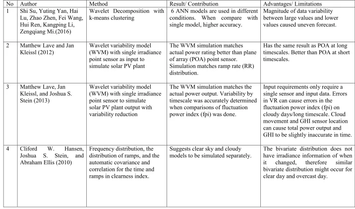
Table 2.2: Review of Previous Studies
No Author Method Result/ Contribution Advantages/ Limitations
1 Shi Su, Yuting Yan, Hai Lu, Zhao Zhen, Fei Wang, Hui Ren, Kangping Li, Zengqiang Mi.(2016)
Wavelet Decomposition with
k-means clustering 6 ANN models are used in different conditions. When compare with single model, higher accuracy.
Magnitude of data variability between large values and lower values caused uneven forecast.
2 Matthew Lave and Jan
Kleissl (2012) Wavelet variability model (WVM) with single irradiance point sensor as input to
simulate solar PV plant
The WVM simulation matches actual power rating better than plane of array (POA) point sensor.
Simulation matches ramp rate (RR) distribution.
Has the same result as POA at long timescales. Better than POA at short timescales.
3 Matthew Lave, Jan Kleissl, and Joshua S. Stein (2013)
Wavelet variability model (WVM) with single irradiance point sensor to simulate solar PV plant output with variability reduction
The WVM simulation matches the actual power output. Variability by timescale was accurately determined when comparisons of fluctuation power index (fpi) was done.
Input requirements only require a single sensor and input data. Errors in VR can cause errors in the fluctuation power index (fpi) on cloudy days/long timescale. Cloud movement and GHI sensor location can cause total power output and GHI to be slightly inaccurate in time. 4 Cliford W. Hansen,
Joshua S. Stein, and Abraham Ellis (2010)
Frequency distribution, the distribution of ramps, and the automatic covariance and correlation for the time and ramps in clearness index.
Suggests clear sky and cloudy
![Table 2.1: Irradiance and solar system power variability [5]](https://thumb-us.123doks.com/thumbv2/123dok_us/67596.6371/19.595.203.405.103.287/table-irradiance-solar-power-variability.webp)