This is a repository copy of Runtime Analysis of Probabilistic Crowding and Restricted
Tournament Selection for Bimodal Optimisation.
White Rose Research Online URL for this paper:
http://eprints.whiterose.ac.uk/130704/
Version: Accepted Version
Proceedings Paper:
Covantes Osuna, E. and Sudholt, D. orcid.org/0000-0001-6020-1646 (2018) Runtime
Analysis of Probabilistic Crowding and Restricted Tournament Selection for Bimodal
Optimisation. In: Proceedings of the Genetic and Evolutionary Computation Conference
(GECCO 2018). Genetic and Evolutionary Computation Conference (GECCO 2018),
15-19 Jul 2018, Kyoto, Japan. ACM . ISBN 978-1-4503-5618-3
https://doi.org/10.1145/3205455.3205591
[email protected] https://eprints.whiterose.ac.uk/ Reuse
Items deposited in White Rose Research Online are protected by copyright, with all rights reserved unless indicated otherwise. They may be downloaded and/or printed for private study, or other acts as permitted by national copyright laws. The publisher or other rights holders may allow further reproduction and re-use of the full text version. This is indicated by the licence information on the White Rose Research Online record for the item.
Takedown
If you consider content in White Rose Research Online to be in breach of UK law, please notify us by
Runtime Analysis of Probabilistic Crowding and
Restricted Tournament Selection for Bimodal Optimisation
Edgar Covantes Osuna and Dirk Sudholt
Department of Computer Science University of Sheffield, United Kingdom
April 18, 2018
Abstract
Many real optimisation problems lead to multimodal domains and so require the identifi-cation of multiple optima. Niching methods have been developed to maintain the population diversity, to investigate many peaks in parallel and to reduce the effect of genetic drift. Using rigorous runtime analysis, we analyse for the first time two well known niching methods: prob-abilistic crowding and restricted tournament selection (RTS). We incorporate both methods into a (µ+1) EA on the bimodal functionTwomaxwhere the goal is to find two optima at opposite ends of the search space. In probabilistic crowding, the offspring compete with their parents and the survivor is chosen proportionally to its fitness. On Twomaxprobabilistic crowding fails to find any reasonable solution quality even in exponential time. In RTS the offspring compete against the closest individual amongst w (window size) individuals. We prove that RTS fails if w is too small, leading to exponential times with high probability. However, ifwis chosen large enough, it finds both optima for Twomaxin time O(µnlogn) with high probability. Our theoretical results are accompanied by experimental studies that match the theoretical results and also shed light on parameters not covered by the theoretical results.
1
Introduction
Premature convergence is one of the major difficulties in Evolutionary Algorithms (EAs), the population converging to a sub-optimal individual before the fitness landscape is explored properly. Real optimisation problems often lead to multimodal domains and so require the identification of multiple optima, either local or global [23,25]. In multimodal optimisation problems, there exist many attractors for which finding a global optimum can become a challenge to any optimisation algorithm. A diverse population can deal with these multimodal problems as it can explore several hills in the fitness landscape simultaneously.
One particular way for diversity maintenance are niching methods, based on the mechanics of natural ecosystems [24]. A niche can be viewed as a subspace in the environment that can support different types of life. A specie is defined as a group of individuals with similar features capable of interbreeding among themselves but that are unable to breed with individuals outside their group. Species can be defined as similar individuals of a specific niche in terms of similarity metrics. In EAs the term niche is used for the search space domain, and species for the set of individuals with similar characteristics.
Most of the analyses and comparisons made between niching methods are assessed by means of empirical investigations using benchmark functions [23,25]. Theoretical runtime analyses have been performed that rigorously quantify the expected time needed to find one or several global optima [2,6,21]. Both approaches are important to understand how these mechanisms impact the EA runtime and if they enhance the search for good individuals. These different expectations imply where EAs and which niching mechanism should be used and, perhaps even more importantly, where they should not be used.
Previous theoretical studies [2,6,21] compared the expected running time of different diversity mechanisms when embedded in a simple baseline EA, the (µ+1) EA. All mechanisms were consid-ered on the well-known bimodal functionTwomax(x) := max{Pn
i=1xi, n− Pn
i=1xi}. Twomax
consists of two different symmetric slopes (or branches)Zeromaxand Onemaxwith 0n and 1n as global optima, respectively, and the goal is to evolve a population that contains both optima1.
Twomaxwas chosen because it is simply structured, hence facilitating a theoretical analysis,
and it is hard for EAs to find both optima as they have the maximum possible Hamming distance. The results allowed for a fair comparison across a wide range diversity mechanisms, revealing that some mechanisms like fitness diversity or avoiding genotype duplicates, perform badly, while other mechanisms like fitness sharing, clearing or deterministic crowding perform surprisingly well (see Table1and Section1.1).
We contribute to this line of work by studying the performance of two classical diversity mech-anisms,probabilistic crowding and restricted tournament selection. Both methods are well-known techniques as covered in tutorials and surveys for diversity-preserving mechanisms [3, 10, 24,26] and compared in empirical investigations [23, 25]. However, we are lacking a good understand-ing of when and why they perform well and how they compare to diversity mechanisms analysed previously.
Inprobabilistic crowding, offspring compete against their most similar parent and the survivor is chosen with a probability proportional to their fitness [13]. The idea is to use a low selection pressure to prevent the loss of niches of lower fitness [13]. Probabilistic crowding has been used for multimodal optimisation [1,13, 14,15], in its plain form as well as in variants in which a scaling factor has been introduced into the replacement policy.
Restricted tournament selection (RTS) is a modification of the classical tournament selection for multimodal optimisation that exhibits niching capabilities. RTS selects two elements from the population uniformly at random (u. a. r.) to undergo recombination and mutation to produce two new offspring. The offspring compete with their closest individual from w (window size) more individuals selected u. a. r. from the population, and the best individual is selected. This form of tournament restricts an entering individual from competing with others too different from it [12]. RTS has been analysed empirically for the classical comparison between crowding mechanisms for multimodal optimisation as a replacement strategy [9, 22]. Recent applications for engineering problems with multimodal domains include facility layout design [8] and the design of product lines [28] with reported better results compared to the other variants without RTS.
Our contribution is to provide a rigorous theoretical runtime analysis for both mechanisms in the context of the (µ+1) EA onTwomax, to rigorously assess their performance in comparison to
other diversity mechanisms. In addition, our goal is to provide insights into the working principles of these mechanisms to enhance our understanding of their strengths and weaknesses.
For the (µ+1) EA with probabilistic crowding, we show in Section 2 that the mechanism is unable to evolve solutions of significantly higher fitness than that obtained during initialisation (or, equivalently, through random search), even when given exponential time. The reason is that fitness-proportional selection between parent and offspring results in an almost uniform choice as both have very similar fitness, hence fitness-proportional selection degrades to uniform selection for replacement. For the (µ+1) EA with restricted tournament selection, we show in Section 3
that the mechanism succeeds in finding both optima ofTwomaxin the same way as deterministic
crowding, provided that the window sizewis chosen large enough. However, if the window size is too small then it cannot prevent one branch taking over the other, leading to exponential running times with high probability.
1In [6] an additional fitness value for 1n
was added to distinguish between a local optimum 0n
Table 1: Overview of runtime analyses for the (µ+1) EA with different diversity mechanisms on
Twomax. Results derived in this paper are shown in bold. The success probability is the
proba-bility of finding both optima within (expected) timeO(µnlogn). Conditions include restrictions on the population sizeµ, the sharing/clearing radiusσ, the niche capacityκ, window sizew, and
µ′:= min(µ,logn). Results from [6] are adapted to our definition of Twomax; see [27] for details.
Diversity Mechanism Success prob. Conditions
Plain (µ+1) EA [6] o(1) µ=o(n/logn) No Duplicates
Genotype [6] o(1) µ=o(√n) Fitness [6] o(1) µ= poly(n) Deterministic Crowding [6] 1−2−µ+1 allµ
Fitness Sharing (σ=n/2)
Population-based [6] 1 µ≥2 Individual-based [21] 1 µ≥3 Clearing (σ=n/2) [2] 1 µ≥κn2
Probabilistic Crowding 2−Ω(n) allµ
RTS
Small w sizes o(1) µ=o(n1/w) Large w sizes 1−2−µ′+3 w≥2.5µlnn
Our theoretical results are accompanied by experiments in Section4 that cover a wider range of parameter settings and that show a very good match between our theoretical and empirical results.
1.1
Previous Work
Table1summarises all known results for diversity mechanisms onTwomax. As can be seen, not
all mechanisms succeed in finding both optima onTwomax efficiently, that is, in expected time
O(µnlogn). Friedrich, Oliveto, Sudholt, and Witt [6] showed that the plain (µ+1) EA and the simple mechanisms likeavoiding genotype or fitness duplicates are not able prevent the extinction of one branch, ending with the population converging to one optimum, with high probability. Deterministic crowding with a sufficiently large population is able to reach both optima with high probability in expected timeO(µnlogn) [6, Theorem 4]. A population-based fitness sharing approach, constructing the best possible new population amongst parents and offspring, with
µ≥2 is able to find both optima in expected optimisation timeO(µnlogn) [6, Theorem 5]. The drawback of this approach is that all possible sizeµsubsets of this union of sizeµ+λ(whereλis the offspring population size) need to be examined. This is prohibitive for largeµandλ.
Oliveto, Sudholt, and Zarges [21] studied the original fitness sharing approach and showed that a population sizeµ= 2 is not sufficient to find both optima in polynomial time; the success probability is only 1/2−Ω(1) [21, Theorem 1]. However, withµ≥3 fitness sharing again finds both optima in expected timeO(µnlogn) [21, Theorem 3]. Covantes Osuna and Sudholt [2] analysed the clearing mechanism and showed that it can optimise all functions of unitation—function defined over the number of 1-bits contained in a string—in expected time O(µnlogn) [2, Theorem 4.4] when the distance function and parameters like the clearing radiusσ, the niche capacity κ(how many winners a niche can support) andµare chosen appropriately. In the case of large niches, that is, with a clearing radius ofσ=n/2, it is able to find both optima in expected time O(µnlogn) [2, Theorem 5.6].
2
Probabilistic Crowding
We start by presenting and analysing the (µ+1) EA using probabilistic crowding, defining it in the same fashion as deterministic crowding in [6]. Recall that in probabilistic crowding, the offspring compete against the most similar parent according to a distance metric and the survivor wins proportionally according to their fitness. Without crossover, this means that the mutanty
competes against its parent x using fitness-proportional selection. Then the probability of the mutanty winning is given by f(xf)+(yf)(y), wheref is the fitness function. The resulting (µ+1) EA is shown in Algorithm1.
Algorithm 1(µ+1) EA with probabilistic crowding
1: Lett:= 0 and initialise P0 withµindividuals chosen u. a. r.
2: whilestopping criterionnotmetdo 3: Choosex∈Pt u. a. r.
4: Createy by flipping each bit inxindependently w/ prob. 1/n. 5: Chooser∈[0,1] u. a. r.
6: if r≤f(yf)+(yf)(x) thenPt+1=Pt\ {x} ∪ {y} elsePt+1=Pt end if
7: t:=t+ 1. 8: end while
There are several related theoretical analyses for fitness-proportional selection for the case of the Onemax function. The Simple Genetic Algorithm (SGA) has been analysed with
fitness-proportional selection for parent selection in [16,19, 20].
Most relevant to this work is the work by Happ, Johannsen, Klein, and Neumann [11], who analysed a variant of the (1 + 1) EA using fitness-proportional selection and showed that it needs exponential time to evolve a fitness of at least (1 +ε)n/2 onOnemaxwith high probability. Their
algorithm can be seen as a special case of the (µ+1) EA with probabilistic crowding for µ= 1. Our result is similar to the result in [11], but it holds for arbitrary population sizesµand it applies to bothOnemaxandTwomax. The proof uses more modern techniques from drift analysis [17]
that were not available to the authors of [11]. In the following lemma we define in expectation how the individual accepted for replacement moves away from the individual selected for mutation.
Lemma 2.1. Let x be the selected parent, y be the offspring, and z ∈ {x, y} be the individual selected for survival. Forf =Onemaxif f(x)≥(1 +δ)n/2 for some positiveδ=δ(n)that may
depend onnthen
E(f(z)−f(x)|x)≤ −δ2+ Θ
1
n
.
The statement also holds for Twomaxiff(x)≥n/2 + logn.
Proof. We first analyse the expected fitness of the mutant y before survival selection. Compared to its parent x, in expectation at least (1 +δ)n/2·1/n = (1 +δ)/2 bits flip from 1 to 0, and at most (1−δ)n/2·1/n= (1−δ)/2 bits flip from 0 to 1. Hence
E(f(y)−f(x)|x)≤(1−δ)/2−(1 +δ)/2 =−δ. (1) We now use this inequality to analyse the fitness differencef(z)−f(x) after survival selection. Observe that this difference is 0 in case z = x. Hence only generations where y is selected for survival contribute to E(f(z)−f(x)|x). The latter can be written as follows.
E(f(z)−f(x)|x)
= ∞
X
d=−∞
Prob(f(y)−f(x) =d|x)·d· f(y)
f(x) +f(y)
Using that withd=f(y)−f(x),
f(y)
f(x) +f(y) =
(f(x) +f(y))/2 +d/2
f(x) +f(y) = 1 2 +
d/2
f(x) +f(y)
= 1 2 + Θ
d
n
we get
E(f(z)−f(x)|x)
= ∞
X
d=−∞
Prob(f(y)−f(x) =d|x)·d·
1
2+ Θ
d n = 1 2 ∞ X
d=−∞
Prob(f(y)−f(x) =d|x)·d
+ Θ 1 n ∞ X
d=−∞
Prob(f(y)−f(x) =d|x)·d2.
The first sum is E(f(y)−f(x))/2 by definition of the expectation, and we already know from (1) that E(f(y)−f(x))/2 ≤ −δ/2. The summands in the second sum can be bounded from above using Prob(f(y)−f(x) = d| x) ≤ 1/(|d|!) as it is necessary to flip at least |d| bits, which has probability at most |nd|
(1/n)|d|≤1/(|d|!). Thus
E(f(z)−f(x)|x)≤ −δ2+ Θ
1
n
∞ X
d=−∞ 1
|d|!·d
2
≤ −δ
2+ Θ
1 n ·2 ∞ X d=1 1
d!·d
2=−δ
2 + Θ
1
n
as P∞ d=1d1! ·d
2 = P∞
d=1(d−d1)! = P∞
d=0d+1d! = P∞
d=0dd! + P∞
d=0d1! = P∞
d=1(d−11)! + P∞
d=0d1! =
2P∞
d=0d1! = 2e.
The statement also holds forTwomaxiff(x)≥n/2 + lognas the algorithm only ever notices
a difference to Onemax in case at least logn bits flip in one mutation. Since this only occurs
with probability at most 1/(logn)! = n−Ω(log logn), and the fitness difference between Onemax
andTwomaxis at mostn/2, this only accounts for an additive error term ofn/2·n−Ω(log logn)=
n−Ω(log logn) in the expectation forOnemax, and this error term is absorbed in the Θ(1/n) term.
Lemma 2.1 gives an important lesson. Assume that the survivalist z was chosen uniformly betweenxandy, then we would have
E(f(z)−f(x)|x) = 1
2 ·E(f(y)−f(x)|x) + 1
2·E(f(x)−f(x)|x) =−
δ
2
using (1) and E(f(x)−f(x)|x) = 0. Lemma 2.1states that compared to this setting, a fitness-proportional selection of z only gives a vanishing bias of Θ(1/n). In other words, Lemma 2.1
quantifies the observation that in the considered context, fitness-proportional selection is very similar to uniform selection. We now use Lemma 2.1 to prove a strong negative result on the performance of the (µ+1) EA with probabilistic crowding. To this end, we will use the negative drift theorem [17,18] (also calledsimplified drift theorem). Note that the expectedOnemaxvalue
of a search point chosen u. a. r. isn/2. It is also easy to show that the expectedTwomax value
of a uniform random search point isn/2 + Θ(√n). These values also represent equilibrium states for sequences of mutations in the absence of selection. The following theorem shows that the (µ+1) EA with probabilistic crowding does not evolve any solutions of significantly higher fitness than these values, even given exponential time.
Theorem 2.2. With probability 1−2−Ω(n) the (µ+1) EA with probabilistic crowding on either
f =Onemaxorf =Twomax will not have found a search point with fitness at least(1 +ε)n/2
in2cn function evaluations, for every population size µ, every constant ε >0 and a small enough constantc >0that may depend onε.
Proof. We assume thatf =Onemaxas Twomaxcan be handled in the same way. We may also
assume thatµ= 2o(n)as ifµ≥2c′n
for any constant 0< c′<1, the statement follows immediately (forc:=c′) as the first 2c′n
most 2·2−n·2c′n
= 2−Ω(n)asc′<1. Note that in the absence of crossover, probabilistic crowding evolvesµindependent lineages as any offspring only competes directly with its parent. We show that the probability of any fixed lineage reaching a fitness of at least (1 +ε)n/2 in 2cngenerations is 2−Ω(n). Taking the union bound over all lineages yields that the probability of reaching such a
fitness is bounded byµ·2−Ω(n)= 2o(n)·2−Ω(n)= 2−Ω(n), which implies the claim.
Now focus on one lineage. By standard Chernoff bounds (see [4]), the probability of initialising the lineage with an initial search point of fitness at least (1 +ε/2)n/2 is 2−Ω(n). If this rare
failure event does not happen, the lineage needs to increase an initial fitness from a value at most (1 +ε/2)n/2 to a value at least (1 +ε)n/2 in order to achieve a fitness of (1 +ε)n/2. We apply the negative drift theorem to the fitness of the current individual in our lineage to show that this does not happen in 2cngenerations with probability 1−2−Ω(n). The interval chosen will be from
a:= (1 +ε/2)n/2 tob:= (1 +ε)n/2; note that it has length εn/4.
Letxbe the selected parent, y be the offspring, andz ∈ {x, y} be the individual selected for survival. We establish the two conditions of the negative drift theorem. The first condition for search points with fitness at leasta= (1 +ε/2)n/2 follows from Lemma2.1withδ:=ε/2, yielding a drift of at most−ε/4 + Θ(1/n) =−Ω(1). The second condition follows easily from properties of standard bit mutation: the fitness difference|f(z)−f(x)|is clearly bounded by the number of flipping bits. The probability of flippingdbits in a standard bit mutation is at most 1/(d!)≤2/2d for alld≥ 1. This proves the second condition when choosingr := 2 and δ:= 1. Invoking the negative drift theorem yields that the probability of one lineage reaching a search point with fitness at least (1 +ε)n/2, starting with a fitness at most (1 +ε/2)n/2, in 2c′εn/2
steps, for some constant
c′>0, is at most 2−Ω(εn/4)= 2−Ω(n). Choosingc:=c′ε/4 completes the proof forOnemax. The same proof can be used for Twomaxwith minor modifications: note that if the number
of ones isk≤n/2, a fitness difference ofdcan be achieved by increasing or decreasing the number of ones byd, providedk+d≤n/2 or by creating an offspring withn−k−dones on the opposite branch. Sincek+d≤n/2≤n−k−d, the probability for the latter event is no larger than that of the former. The same holds symmetrically fork≥n/2. Hence all transition probabilities are bounded by twice the previous bound forOnemax and the second condition can be fulfilled by
doublingrand choosingc:=c′ε/8. Then the result follows as forOnemax.
3
Restricted Tournament Selection
The (µ+1) EA with restricted tournament selection (RTS) is defined in a similar way. Recall that in RTS a new offspring competes with the closest element fromw (window size) more members selected u. a. r. from the population, and the better individual from this competition is selected.
In the (µ+1) EA with RTS, shown in Algorithm2, an individualxis selected u. a. r. as a parent and a new individualyis created in the mutation step. Since we are not considering crossover and only one individual is created,windividuals are selected u. a. r. with replacement and stored in a temporary populationP∗
t. Then in Line6an individualzis selected from populationPt∗ with the minimum distance fromy (ties are broken u. a. r.), and if the individualy has a fitness at least as good asz,y replacesz.
Algorithm 2(µ+1) EA with restricted tournament selection 1: Lett:= 0 and initialise P0 withµindividuals chosen u. a. r.
2: whilestopping criterionnotmetdo 3: Choosex∈Pt u. a. r.
4: Createy by flipping each bit inxindependently w/ prob. 1/n. 5: Selectwindividuals u. a. r. fromPtand store them inPt∗. 6: Choosez∈P∗
t such that min z∈P∗
t
d(y, z).
7: if f(y)≥f(z)thenPt+1=Pt\ {z} ∪ {y}else Pt+1=Pt end if 8: t:=t+ 1.
9: end while
As distance functions d we consider genotypic or Hamming distance, defined as the number of bits that have different values inx and y: d(x, y) := H(x, y) := Pn−1
i=0 |xi−yi|, and phenotypic
distances as in [2,6, 21] based on the number of ones: d(x, y) :=| |x|1− |y|1|where |x|1 and|y|1
3.1
Large Window Sizes Are Effective
Now, let us start with the theoretical analysis forTwomax with a positive result for RTS. The
following shows that, ifw is chosen very large, the (µ+1) EA with RTS behaves almost like the (µ+1) EA with deterministic crowding.
Theorem 3.1. If µ =o(√n/logn) and w ≥ 2.5µlnn then the (µ+1) EA with restricted tour-nament selection using genotypic or phenotypic distance finds both optima on Twomax in time
O(µnlogn) with probability at least1−2−µ′+3
, whereµ′:= min(µ,logn).
Note that the probability 1−2−µ′+3
is close to the success probability 1−2−µ+1for
determin-istic crowding, ifµ≤logn, apart from a constant factor in front of the 2−µ′
term. For both, the success rate converges to 1 very quickly for increasing population sizes. For restricted tournament selection our probability bound is capped at 1−2−logn+3 = 1−8/n as there is always a small
probability of an unexpected takeover occurring.
In order to prove Theorem3.1, we first analyse the probability of initialising a population such that there are individuals on each branch with a safety gap ofσto the border between branches. This safety gap will be used to exclude the possibility that the best individual on one branch creates offspring on the opposite branch.
Lemma 3.2. Consider the population of the (µ+1) EAon Twomaxand for some µandσ. The
probability of having at least one initial search point with at most n/2−σ ones and one search point with at leastn/2 +σones is at least
1−2 1 + 2σ·
p
2/n
2
!µ
≥1−2−µ+1(1 +o(1))
where the inequality holds ifσµ=o(√n).
Proof. Using [4, Lemma 7], for a random variable with binomial distribution Bin(n,1/2), for all
z∈[0, n] we have
Prob(X =z)≤Prob(X =⌊n/2⌋)≤2−n·
n
⌊n/2⌋
≤p2/n.
So let us start by defining the probability that an individual xis initialised inside the safety gap is at most
pσ := Prob(n/2−σ <|x|1< n/2 +σ)≤2σ· p
2/n.
Now let us define the probability that an individual x is initialised on the outer regions with
|x|1≤n/2−σones (0nbranch) or|x|1≤n/2 +σones (1nbranch) asp0andp1, respectively. Note
that bothp0andp1are symmetric, andp0+p1:= 1−pσ, and by rewriting we obtainp0:= 1−2pσ
(the same forp1) with its complement being 1−1−2pσ = 1+2pσ.
So the probability of having no individual with at mostn/2−σ ones is (1−p1)µ= 1+2pσ µ
, and the same holds for having no individual with at leastn/2 +σ ones. Hence the probability of being initialised as stated in the statement of the lemma is at least
1−2
1 +p σ 2
µ
= 1−2−µ+1·(1 +pσ)µ.
Plugging inpσ and using the inequality 1 +x≤exas well asσµ=o(√n) we simplify the last term as
(1 +pσ)µ ≤e2σµ
√
2/n=eo(1)= 1
e−o(1) ≤
1
1−o(1) = 1 +o(1), and by plugging all together we have 1−2−µ+1(1 +o(1)).
We also show the following time bound, which assumes that the (µ+1) EA never decreases the best fitness on a considered branch. We will later show in the proof of Theorem3.1 that this assumption is met with high probability.
Lemma 3.3. Consider one branch of Twomax and a (µ+1) EA with a replacement selection
Proof. We apply the multiplicative drift theorem with tail bounds [5] to random variables Xt that describe the Hamming distance of the closest individual to the targeted optimum. Note that
X0 ≤ n/2 as we start with an individual on the considered branch and the optimum has been
found onceXt= 0.
The probability of selecting an individual with Hamming distanceXtis at least 1/µ. In order to create a better individual, it is sufficient that one of the Xt differing bits is flipped and the other bits remain unchanged. Each bit flip has a probability of being mutated of 1/n and the remaining bits remain unchanged with probability (1−1/n)n−1. Hence, the probability of creating
an individual with a smaller Hamming distance is bounded as follows:
Prob(Xt+1< Xt|Xt)≥ 1
µ· Xt
n ·
1−1
n
n−1
≥ Xt
µen.
This implies
E(Xt+1|Xt)≤
1−eµn1
Xt.
Applying Theorem 1 in [5] yields that the time till the optimum is found is at mosteµn·(ln(n/2) + lnn)≤2eµnlnnwith probability at most 1/nand in expectation.
Using these two lemmas, we can now prove Theorem3.1.
Proof of Theorem3.1. According to Lemma 3.2, with probability 1−2−µ+1(1 +o(1)) the initial
population contains at least one search point with at mostn/2−lognones and at least one search point with at leastn/2 + logn ones. We assume in the following that this has happened. The probability of mutation flipping at least lognbits is at most 1/(logn)! =n−Ω(log logn). Taking the
union bound overO(µnlogn) steps still gives a superpolynomially small error probability. In the following, we work under the assumption that mutation never flips more than lognbits.
We call two search pointsclose if their genotypic distance is at most logn. Due to our assump-tion on mutaassump-tions, every newly created offspring is close to its parent. Note that onTwomax
the phenotypic distance of any two search point is bounded from above by the genotypic distance, hence close search points also have a phenotypic distance of at most logn. Note that, whenever the tournament contains a search point that is close to the new offspring, either the offspring or a close search point will be removed. If this always happens, the best individual on any branch cannot be eliminated by an offspring on the opposite branch; recall that initially, the best search points on the two branches have phenotypic distance at least 2 logn, and this phenotypic distance increases if the best fitness on any branch improves. When genotypic distances are being used, the genotypic distance is always at least 2 logn.
Since each offspring has at least one close search point (its parent), the probability that the tournament does not contain any close search point is at most (1−1/µ)w ≤e−w/µ =e−2.5 lnn = 1/n2.5. So long as the best individual on any branch does not get replaced by any individuals on
the opposite branch, the conditions of Lemma3.3are met. Applying Lemma3.3to both branches, by the union bound the probability of both optima being found in time 2eµnlnnis at least 1−2/n. The probability that in this time a tournament occurs that does not involve a close search point isO(µnlogn)·1/n2.5=o(1/n) asµ=o(√n/logn).
All failure probabilities sum up to (assumingnlarge enough)
2
n+o
1
n
+ 2−µ+1(1 +o(1)) + O(µnlogn)
n−Ω(log logn) ≤
4
n+ 2
−µ+2
≤2−µ′+3
where the last inequality follows as 2−µ ≤2−µ′
and 1/n≤2−µ′
.
In Theorem3.1we chosewso large that every tournament included the offspring’s parent with high probability. Then the (µ+1) EA behaves like the (µ+1) EA with deterministic crowding [6], leading to similar success probabilities (see Table1).
A success probability around 1−2−µ+1 is best possible for many diversity mechanisms as
with probability 2−µ+1 the whole population is initialised on one branch only (for odd n), and
3.2
Small Window Sizes Can Fail
We now turn our attention to small w. If the w is small in comparison to µ, the possibility emerges that the tournament only contains individuals that are far from the offspring. In that case even the closest individual in the tournament will be dissimilar to the offspring, resulting in a competition between individuals from different “niches” (i. e., sets of similar individuals). The following theorem and its proof show that this may result in one branch taking over the other branch, even when the branch to get extinct is very close to a global optimum. The resulting expected optimisation time is exponential.
Theorem 3.4. Let µ ≤ n/8. The probability that the (µ+1) EA with restricted tournament selection withw≥2 and either genotypic or phenotypic distances finds both optima on Twomax
in timenn−1 is at most O(µw/n). If µ≤εn1/w for a sufficiently small constantε > 0 then the expected time for finding both optima isΩ(nn).
Note that the probability of finding both optima innn−1 generations is o(1) if w=O(1) and
µgrows slower than the polynomial n1/w. It also holds if w≤c(lnn)/ln lnn for some constant 0 < c <1 and µ =O(logn) as then n1/w =e(lnn)/w ≥e(ln lnn)/c = (lnn)1/c =ω(logn), which showsµw/n=o(1).
Proof of Theorem3.4. The analysis follows the proof of [6, Theorem 1]. We assume that the initial population contains at most one global optimum as the probability of both optima being found during initialization is at mostµ·2−n=O(µw/n).
We consider the first point of time at which the first optimum is being bound. Without loss of generality, let us assume that this is 0n. Then we show that with high probability copies of 0n take over the population before the other optimum 1n is found.
Let i be the number of copies of the 0n individuals in the population, then a good event G i (good in a sense of leading towards extinction as we are aiming at a negative result) is to increase this number fromitoi+ 1. For this it is just necessary to create copies of one of theiindividuals. For n ≥ 2 we have Prob(Gi) ≥ µi · 1−1n
n
·µ−µi w
≥ 4iµ · µ−i
µ w
since it suffices to select one out of i individuals and to create a copy of the selected individual, and to select w times individuals from the remainingµ−i individuals. On the other hand, a bad eventBi is to create an 1n individual in one generation. This probability is clearly bounded by Prob(B
i)≤ 1n as every individual with at least one zero bit has to flip said bit to create 1n. Together, the probability that the good eventGi happens before the bad eventBi is
Prob(Gi|Gi∪Bi)≥ Prob(Gi)
Prob(Gi) + Prob(Bi)≥ i 4µ ·
µ−i
µ w
i 4µ·
µ−i
µ w
+1 n
= 1−
1 n i 4µ·
µ−i µ
w
+1n ≥
1− 4µ
in·((µ−i)/µ)w.
The probability that theiindividuals take over the population before 1n is found is therefore at least
µ Y
i=1
Prob(Gi|Gi∪Bi)≥ µ Y
i=1
1−in 4µ ·((µ−i)/µ)w
.
Using 4nµ ≤ 1
2 and 1−x≥e
−2xforx≤1
2, we obtain
µ Y
i=1
1−in 4µ ·((µ−i)/µ)w
≥ µ Y i=1 exp
−in 8µ ·((µ−i)/µ)w
= exp −8nµ ·
µ−1 X
i=1
1
i·((µ−i)/µ)w !
= exp −8nµ ·µw
µ−1 X
i=1
1
i·(µ−i)w
!
Note that the summands are non-increasing withw. So the worst case is having the smallest possiblew≥2, so we can bound this sum from above in the following way:
µ−1 X
i=1
1
i·(µ−i)2 ≤
⌊µ/2⌋
X
i=1
1
i·(µ−i)2 + µ−1 X
i=⌈µ/2⌉ 1
i·(µ−i)2
≤
⌊µ/2⌋
X
i=1
1
i·(µ/2)2 + µ−1 X
i=⌈µ/2⌉
1
µ/2·(µ−i)2
≤ µ42
⌊µ/2⌋
X i=1 1 i + 2 µ ∞ X i=1 1
i2 =O 1
µ
asP⌊µ/2⌋
i=1 1i =O(logµ) and P∞
i=11/i2=π2/6. Together we have
µ Y
i=1
Prob(Gi|Gi∪Bi)≥exp
−8nµ·µw·O
1
µ
≥1−O
µw
n
.
Once the population consists only of copies of 0n, a mutation has to flip allnbits to find the 1n optimum. This event has probability n−n and, by the union bound, the probability of this happening in a phase consisting ofnn−1 generations is at most 1
n = O(µw/n). The sum of all failure probabilities isO(µw/n), which proves the first claim. For the second claim, observe that the conditional expected optimization time isnn once the population has collapsed to copies of 0n individuals. As this situation occurs with probability at least 1−O(µw/n) = Ω(1) if the constant
εinµ≤εn1/w is sufficiently small, the unconditional expected optimization time is Ω(nn).
4
Experiments
We provide an experimental analysis as well in order to see how closely the theory matches the empirical performance for reasonable problem sizes, and to investigate a wider range of parameters, where the theoretical results are not applicable. Our analysis is focused on the (µ+1) EA with probabilistic crowding and RTS for theTwomaxfunction. We consider exponentially increasing
population sizesµ={2,4,8, . . . ,1024} for a problem sizen= 100 and for 100 runs.
Since we are interested in proving how good/bad all algorithms are, we define the following outcomes and stopping criteria for each run. Success, both optima ofTwomaxhave been reached,
i. e., the run is stopped if the population contains both 0n and 1n in the population. Failure, once the run has reached 10µnlnngenerations and the population does not contain both optima. By Lemma3.3, this time period is long enough to allow any reasonable (µ+1) EA variant to find one or two global optima with high probability (unless the best fitness on a branch drops frequently). We report the mean of successes and failures for the 100 runs.
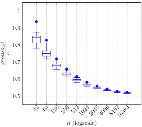
For probabilistic crowding (Algorithm 1), and as proved in Theorem 2.2, for all µ sizes, the method is not able to optimise Twomax. In all runs the algorithm failed to reach even one
optimum, let alone reaching both. Since the algorithm is not able to find any optimum ofTwomax,
we ran additional experiments for n = {32,64,128, . . . ,16384} and population size µ = 32 to observe how far the best lineages evolve from n/2 and/or how close the best individuals get to reach an optimum. In Figure1, we show the best individuals obtained in each of the 100 runs and its variance. As soon asnincreases, the best fitness in the population starts to concentrate around
n/2 and reaching a fitness of (1 +ε)n/2 becomes very difficult for all constantsε >0 asngrows. Even the best outliers start to get closer and closer to the average of the population.
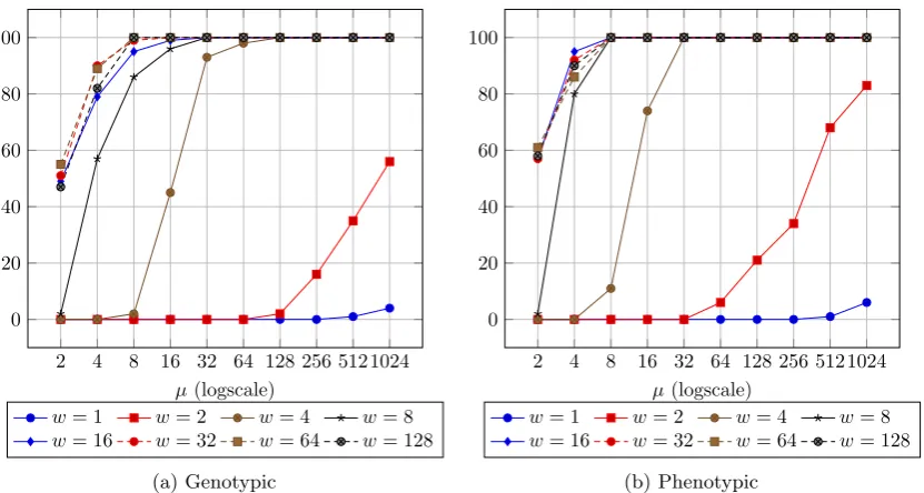
In the case of RTS (Algorithm2), we ran experiments forw={1,2,4,8, . . . ,1024}, however we only plot results up tow= 128 as the results for large wwere very similar. Figure 2 shows that for small values ofwand µthe algorithm is not able to maintain individuals on both branches of
Twomaxfor a long period of time, as predicted by Theorem3.4. It is only when the population
32 64 128 256 5121024 2048 4096 819216384 0.5
0.6 0.7 0.8 0.9 1
n (logscale)
T
w
o
m
a
x
(
y
)
[image:12.595.176.423.81.301.2]n
Figure 1: The normalised best fitness Twomax/n reached among 100 runs at the time both
optima were found or the t = 10µnlnn generations have been reached on Twomax for n =
{32,64,128, . . . ,16384} by the (µ+1) EA with probabilistic crowding withµ= 32.
O(µw/n) from Theorem3.4. Our experiments show that RTS works well for much smaller window sizes than those required in Theorem3.1. As a final remark, the method seems to behave fairly similarly with respect to both distance functions.
5
Conclusions
We have examined theoretically and empirically the behaviour of two different niching mechanisms embedded into a simple (µ+1) EA onTwomax. We rigorously proved that probabilistic crowding
fails miserably; it is not even able to evolve search points that are significantly better than those found by random search, even when given exponential time. The reason is that fitness-proportional selection for survival selection works very similar to uniform selection, and then the algorithm performs an almost blind search onµindependent lineages.
Our results highlight the importance of scaling the fitness, as done in [1, 14, 15]. An open question is whether fitness scaling would enable probabilistic crowding to find both optima on
Twomax, and if so, how much the fitness needs to be scaled. A proof where fitness scaling has
helped for a variant of the Simple GA onOnemaxwas given in [16]. We are confident that the
proof arguments used here can also be used to analyse more advanced versions of crowding [7,15]. The performance of restricted tournament selection seems to vary a lot with the parameters involved. We have shown that ifµ andw are set too small, one subpopulation may get extinct. But if w is large enough then RTS behaves similarly to deterministic crowding. For both the probability of finding both optima is close to 1−2−µ+1, hence converging to 1 very quickly as
µ grows. It still an open problem to theoretically analyse the population dynamics of RTS for intermediate values forw. Our experiments show that RTS can optimiseTwomaxfor smallerw
than the one required in Theorem3.1.
Acknowledgements
2 4 8 16 32 64 128 256 5121024 0
20 40 60 80 100
µ(logscale)
w= 1 w= 2 w= 4 w= 8
w= 16 w= 32 w= 64 w= 128
(a) Genotypic
2 4 8 16 32 64 128 256 5121024
0 20 40 60 80 100
µ(logscale)
w= 1 w= 2 w= 4 w= 8
w= 16 w= 32 w= 64 w= 128
[image:13.595.95.511.81.303.2](b) Phenotypic
Figure 2: The number of successful runs measured among 100 runs at the time both optima were found onTwomaxort= 10µnlnngenerations have been reached forn= 100 with the (µ+1) EA
with restricted tournament selection with µ ={2,4,8, . . . ,1024}, w = {1,2,4,8, . . . ,128}, geno-typic and phenogeno-typic distance.
References
[1] P. J. Ballester and J. N. Carter. An effective real-parameter genetic algorithm with parent centric normal crossover for multimodal optimisation. InProceedings of the Genetic and Evo-lutionary Computation Conference, GECCO ’04, pages 901–913. Springer Berlin Heidelberg, 2004. ISBN 978-3-540-24854-5.
[2] E. Covantes Osuna and D. Sudholt. Analysis of the clearing diversity-preserving mechanism. InProceedings of the 14th ACM/SIGEVO Conference on Foundations of Genetic Algorithms, FOGA ’17, pages 55–63. ACM, 2017. ISBN 978-1-4503-4651-1. doi: 10.1145/3040718.3040731.
[3] M. ˇCrepinˇsek, S.-H. Liu, and M. Mernik. Exploration and exploitation in evolutionary al-gorithms: A survey. ACM Comput. Surv., 45(3):35:1–35:33, 2013. ISSN 0360-0300. doi: 10.1145/2480741.2480752.
[4] B. Doerr. Probabilistic Tools for the Analysis of Randomized Optimization Heuristics. ArXiv e-prints, Jan. 2018.
[5] B. Doerr and L. A. Goldberg. Drift analysis with tail bounds. InParallel Problem Solving from Nature, PPSN XI, pages 174–183. Springer Berlin Heidelberg, 2010. ISBN 978-3-642-15844-5.
[6] T. Friedrich, P. S. Oliveto, D. Sudholt, and C. Witt. Analysis of Diversity-preserving Mech-anisms for Global Exploration. Evolutionary Computation, 17(4):455–476, 2009. ISSN 1063-6560. doi: 10.1162/evco.2009.17.4.17401.
[7] S. F. Galan and O. J. Mengshoel. Generalized crowding for genetic algorithms. InProceedings of the 12th Annual Conference on Genetic and Evolutionary Computation, GECCO ’10, pages 775–782, New York, NY, USA, 2010. ACM. ISBN 978-1-4503-0072-8. doi: 10.1145/1830483. 1830620.
[8] L. Garc´ıa-Hern´andez, J. M. Palomo-Romero, L. Salas-Morera, A. Arauzo-Azofra, and H. Pier-reval. A novel hybrid evolutionary approach for capturing decision maker knowledge into the unequal area facility layout problem. Expert Systems with Applications, 42(10):4697–4708, 2015. ISSN 0957-4174. doi: 10.1016/j.eswa.2015.01.037.
[10] N. N. Glibovets and N. M. Gulayeva. A review of niching genetic algorithms for multimodal function optimization. Cybernetics and Systems Analysis, 49(6):815–820, 2013. ISSN 1573-8337. doi: 10.1007/s10559-013-9570-8.
[11] E. Happ, D. Johannsen, C. Klein, and F. Neumann. Rigorous analyses of fitness-proportional selection for optimizing linear functions. In Proceedings of the Genetic and Evolutionary Computation Conference, GECCO ’08, pages 953–960. ACM, 2008. ISBN 978-1-60558-130-9. doi: 10.1145/1389095.1389277.
[12] G. R. Harik. Finding Multimodal Solutions Using Restricted Tournament Selection. In Pro-ceedings of the 6th International Conference on Genetic Algorithms, pages 24–31. Morgan Kaufmann Publishers Inc., 1995. ISBN 1-55860-370-0.
[13] O. Mengsheol and D. Goldberg. Probabilistic crowding: Deterministic crowding with proba-bilistic replacement. InProceedings of the Genetic and Evolutionary Computation Conference, GECCO ’99, pages 409–416, 1999.
[14] O. J. Mengshoel and D. E. Goldberg. The crowding approach to niching in genetic algorithms. Evol. Comput., 16(3):315–354, 2008. ISSN 1063-6560. doi: 10.1162/evco.2008.16.3.315.
[15] O. J. Mengshoel, S. F. Gal´an, and A. de Dios. Adaptive generalized crowding for genetic algorithms. Information Sciences, 258:140–159, 2014. ISSN 0020-0255. doi: 10.1016/j.ins. 2013.08.056.
[16] F. Neumann, P. S. Oliveto, and C. Witt. Theoretical analysis of fitness-proportional selec-tion: Landscapes and efficiency. In Proceedings of the Genetic and Evolutionary Computa-tion Conference, GECCO ’09, pages 835–842. ACM, 2009. ISBN 978-1-60558-325-9. doi: 10.1145/1569901.1570016.
[17] P. S. Oliveto and C. Witt. Simplified drift analysis for proving lower bounds in evolutionary computation. Algorithmica, 59(3):369–386, 2011.
[18] P. S. Oliveto and C. Witt. Erratum: Simplified Drift Analysis for Proving Lower Bounds in Evolutionary Computation. ArXiv e-prints, 2012.
[19] P. S. Oliveto and C. Witt. On the runtime analysis of the simple genetic algorithm.Theoretical Computer Science, 545:2–19, 2014. ISSN 0304-3975. doi: 10.1016/j.tcs.2013.06.015. Genetic and Evolutionary Computation.
[20] P. S. Oliveto and C. Witt. Improved time complexity analysis of the simple genetic algorithm. Theoretical Computer Science, 605:21–41, 2015. ISSN 0304-3975. doi: 10.1016/j.tcs.2015.01. 002.
[21] P. S. Oliveto, D. Sudholt, and C. Zarges. On the Runtime Analysis of Fitness Sharing Mech-anisms. InParallel Problem Solving from Nature – PPSN XIII, volume 8672 ofLecture Notes in Computer Science, pages 932–941. Springer International Publishing, 2014. ISBN 978-3-319-10761-5. doi: 10.1007/978-3-319-10762-2 92.
[22] B. Y. Qu and P. N. Suganthan. Novel multimodal problems and differential evolution with ensemble of restricted tournament selection. InIEEE Congress on Evolutionary Computation, pages 1–7, 2010. doi: 10.1109/CEC.2010.5586341.
[23] B. Sareni and L. Krahenbuhl. Fitness sharing and niching methods revisited. IEEE Transactions on Evolutionary Computation, 2(3):97–106, Sep 1998. ISSN 1089-778X. doi: 10.1109/4235.735432.
[24] O. M. Shir. Niching in evolutionary algorithms. In Handbook of Natural Computing, pages 1035–1069. Springer Berlin Heidelberg, 2012. ISBN 978-3-540-92910-9. doi: 10.1007/ 978-3-540-92910-9 32.
[26] G. Squillero and A. Tonda. Divergence of character and premature convergence: A survey of methodologies for promoting diversity in evolutionary optimization. Information Sciences, 329:782–799, 2016. ISSN 0020-0255. doi: 10.1016/j.ins.2015.09.056. Special issue on Discovery Science.
[27] D. Sudholt. The Benefits of Population Diversity in Evolutionary Algorithms: A Survey of Rigorous Runtime Analyses. ArXiv e-prints, Jan. 2018.