https://doi.org/10.5194/gmd-11-1033-2018 © Author(s) 2018. This work is distributed under the Creative Commons Attribution 3.0 License.
The PMIP4 contribution to CMIP6 – Part 1: Overview and
over-arching analysis plan
Masa Kageyama1, Pascale Braconnot1, Sandy P. Harrison2, Alan M. Haywood3, Johann H. Jungclaus4, Bette L. Otto-Bliesner5, Jean-Yves Peterschmitt1, Ayako Abe-Ouchi6,7, Samuel Albani1,8, Patrick J. Bartlein9, Chris Brierley10, Michel Crucifix11, Aisling Dolan3, Laura Fernandez-Donado12, Hubertus Fischer13,
Peter O. Hopcroft14,15, Ruza F. Ivanovic3, Fabrice Lambert16, Daniel J. Lunt14, Natalie M. Mahowald17,
W. Richard Peltier18, Steven J. Phipps19, Didier M. Roche1,20, Gavin A. Schmidt21, Lev Tarasov22, Paul J. Valdes14, Qiong Zhang23, and Tianjun Zhou24
1Laboratoire des Sciences du Climat et de l’Environnement, LSCE/IPSL, CEA-CNRS-UVSQ, Université Paris-Saclay, 91191 Gif-sur-Yvette, France
2Centre for Past Climate Change and School of Archaeology, Geography and Environmental Science (SAGES) University of Reading, Whiteknights, RG6 6AH, Reading, UK
3School of Earth and Environment, University of Leeds, Woodhouse Lane, Leeds, LS2 9JT, UK 4Max Planck Institute for Meteorology, Bundesstrasse 53, 20146 Hamburg, Germany
5National Center for Atmospheric Research, 1850 Table Mesa Drive, Boulder, CO 80305, USA
6Atmosphere Ocean Research Institute, University of Tokyo, 5-1-5, Kashiwanoha, Kashiwa-shi, Chiba 277-8564, Japan 7Japan Agency for Marine-Earth Science and Technology, 3173-25 Showamachi, Kanazawa, Yokohama,
Kanagawa, 236-0001, Japan
8Institute for Geophysics and Meteorology, University of Cologne, Cologne, Germany 9Department of Geography, University of Oregon, Eugene, OR 97403-1251, USA 10University College London, Department of Geography, WC1E 6BT, UK
11Université catholique de Louvain, Earth and Life Institute, Louvain-la-Neuve, Belgium 12Dpto. Física de la Tierra, Astronomía y Astrofísica II, Instituto de Geociencias (CSIC-UCM), Universidad Complutense de Madrid, Spain
13Climate and Environmental Physics, Physics Institute & Oeschger Centre for Climate Change Research, University of Bern, Sidlerstrasse 5, 3012 Bern, Switzerland
14School of Geographical Sciences, University of Bristol, Bristol, UK
15School of Geography, Earth & Environmental Sciences, University of Birmingham, Birmingham, UK 16Catholic University of Chile, Department of Physical Geography, Santiago, Chile
17Department of Earth and Atmospheric Sciences, Bradfield 1112, Cornell University, Ithaca, NY 14850, USA 18Department of Physics, University of Toronto, 60 St. George Street, Toronto, Ontario M5S 1A7, Canada
19Institute for Marine and Antarctic Studies, University of Tasmania, Private Bag 129, Hobart, TAS 7001, Australia 20Earth and Climate Cluster, Faculty of Science, Vrije Universiteit Amsterdam, Amsterdam, the Netherlands 21NASA Goddard Institute for Space Studies and Center for Climate Systems Research, Columbia University 2880 Broadway, New York, NY 10025, USA
22Department of Physics and Physical Oceanography, Memorial University of Newfoundland and Labrador, St. John’s, NL, A1B 3X7, Canada
23Department of Physical Geography, Stockholm University, Stockholm, Sweden
24LASG, Institute of Atmospheric Physics, Chinese Academy of Sciences, P.O. Box 9804, Beijing 100029, China
Correspondence:Masa Kageyama ([email protected]) Received: 1 May 2016 – Discussion started: 26 May 2016
Abstract. This paper is the first of a series of four GMD papers on the PMIP4-CMIP6 experiments. Part 2 (Otto-Bliesner et al., 2017) gives details about the two PMIP4-CMIP6 interglacial experiments, Part 3 (Jungclaus et al., 2017) about the last millennium experiment, and Part 4 (Kageyama et al., 2017) about the Last Glacial Maximum ex-periment. The mid-Pliocene Warm Period experiment is part of the Pliocene Model Intercomparison Project (PlioMIP) – Phase 2, detailed in Haywood et al. (2016).
The goal of the Paleoclimate Modelling Intercomparison Project (PMIP) is to understand the response of the climate system to different climate forcings for documented climatic states very different from the present and historical climates. Through comparison with observations of the environmen-tal impact of these climate changes, or with climate recon-structions based on physical, chemical, or biological records, PMIP also addresses the issue of how well state-of-the-art numerical models simulate climate change. Climate models are usually developed using the present and historical cli-mates as references, but climate projections show that fu-ture climates will lie well outside these conditions. Palaeo-climates very different from these reference states there-fore provide stringent tests for state-of-the-art models and a way to assess whether their sensitivity to forcings is com-patible with palaeoclimatic evidence. Simulations of five different periods have been designed to address the objec-tives of the sixth phase of the Coupled Model Intercom-parison Project (CMIP6): the millennium prior to the in-dustrial epoch (CMIP6 name:past1000); the mid-Holocene, 6000 years ago (midHolocene); the Last Glacial Maximum, 21 000 years ago (lgm); the Last Interglacial, 127 000 years ago (lig127k); and the mid-Pliocene Warm Period, 3.2 mil-lion years ago (midPliocene-eoi400). These climatic periods are well documented by palaeoclimatic and palaeoenviron-mental records, with climate and environpalaeoenviron-mental changes rel-evant for the study and projection of future climate changes. This paper describes the motivation for the choice of these periods and the design of the numerical experiments and database requests, with a focus on their novel features com-pared to the experiments performed in previous phases of PMIP and CMIP. It also outlines the analysis plan that takes advantage of the comparisons of the results across periods and across CMIP6 in collaboration with other MIPs.
1 Introduction
Instrumental meteorological and oceanographic data show that the Earth has undergone a global warming of ∼0.85◦C since the beginning of the Industrial Revolution (Hartmann et al., 2013), largely in response to the increase in atmo-spheric greenhouse gases. Concentrations of atmoatmo-spheric greenhouse gases are projected to rise significantly during
the 21st century, reaching levels well outside the range of recent millennia. In making future projections, models are operating beyond the conditions under which they have been developed and validated. Changes in the recent past provide only limited evidence for how climate responds to changes in external factors and internal feedbacks of the magnitude ex-pected in the future. Palaeoclimate states radically different from those of the recent past provide a way to test model per-formance outside the range of recent climatic variations and to study the role of forcings and feedbacks in establishing these climates. Although palaeoclimate simulations strive for verisimilitude in terms of forcings and the treatment of feed-backs, none of the models used for future projection have been developed or calibrated to reproduce past climates.
We have to look back 3 million years to find a period of Earth’s history when atmospheric CO2concentrations were similar to the present day (the mid-Pliocene Warm Period, mPWP). We have to look back several tens of millions of years further (the early Eocene, ∼55 to 50 million years ago) to find CO2 concentrations similar to those projected for the end of this century. These periods can offer key in-sights into climate processes that operate in a higher CO2, warmer world, although their geographies are different from today (e.g. Lunt et al., 2012; Caballero and Huber, 2010). During the Quaternary (2.58 million years ago to present), Earth’s geography was similar to today and the main exter-nal factors driving climatic changes were the variations in the seasonal and latitudinal distribution of incoming solar energy arising from cycles in Earth’s orbit around the Sun. The feed-backs from changes in greenhouse gas concentrations and ice sheets acted as additional controls on the dynamics of the atmosphere and the ocean. In addition, rapid climate transi-tions, on human-relevant timescales (decades to centuries), have been documented for this most recent period (e.g. Mar-cott et al., 2014; Steffensen et al., 2008).
regional climates, and local environmental responses to these changes during climate periods when the relative importance of various climate feedbacks cannot be assumed to be sim-ilar to today. This challenge is paralleled by concerns about future local or regional climate changes and their impact on the environment. Therefore, modelling palaeoclimates is a means to understand past climate and environmental changes better, using physically based tools, as well as a means to evaluate model skill in forecasting the responses to major drivers.
These challenges are at the heart of the Paleoclimate Mod-eling Intercomparison Project (PMIP) and the new set of CMIP6-PMIP4 simulations (Otto-Bliesner et al., 2017; Jung-claus et al., 2017; Kageyama et al., 2017; Haywood et al., 2016) has the ambition of tackling them. Palaeoclimate ex-periments for the Last Glacial Maximum, the mid Holocene, and the last millennium were formally included in CMIP dur-ing its fifth phase (CMIP5, Taylor et al., 2012), equivalent to the third phase of PMIP (PMIP3, Braconnot et al., 2012). This formal inclusion made it possible to compare the mech-anisms causing past and future climate changes in a rigorous way (e.g. Izumi et al., 2015) and to evaluate the models used for projections (e.g. Harrison et al., 2014, 2015). More than 20 modelling groups took part in PMIP3 and many of the PMIP3 results are prominent in the fifth IPCC assessment report (Masson-Delmotte et al., 2013; Flato et al., 2013). PMIP3 also identified significant knowledge gaps and areas where progress is needed. PMIP4 has been designed to ad-dress these issues.
The five periods chosen for PMIP4-CMIP6 (Table 1) were selected because they contribute directly to the CMIP6 ob-jectives; in particular, they address the key CMIP6 question “How does the Earth system respond to forcing?” (Eyring et al., 2016) for multiple forcings and climate states different from the current or historical climates. They are character-ized by greenhouse gas concentrations, astronomical param-eters, ice sheet extent and height, and volcanic and solar ac-tivities different from the current or historical ones (Table 2). This is consistent with the need to provide a large sample of the climate responses to important forcings. The choice of two new periods, the Last Interglacial (LIG,∼127 000 years ago) and the mid-Pliocene Warm Period, was motivated by the desire to explore the relationships between the climate– ice sheet system and sea level and to expand analyses of cli-mate sensitivity and polar amplification. For each target pe-riod, comparison with environmental observations and cli-mate reconstructions enables us to determine whether the modelled responses are realistic, allowing PMIP to address the second key CMIP6 question “What are the origins and consequences of systematic model biases?”. PMIP simula-tions and data–model comparisons will show whether or not the biases in the present-day simulations are found in other climate states. Also, analyses of PMIP simulations will show whether or not present-day biases have an impact on the mag-nitude of simulated climate changes. Finally, PMIP is also
relevant to the third CMIP6 question “How can we assess fu-ture climate changes given climate variability, predictability, and uncertainties in scenarios?” because the simulation of the last millennium’s climate includes more processes (e.g. vol-canic and solar forcings) to describe natural climate variabil-ity than thepiControlexperiment.
The detailed justification of the experimental protocols and analysis plans for each period are given in a series of companion papers: Otto-Bliesner et al. (2017) for the mid-Holoceneandlig127kaexperiments, Kageyama et al. (2017) for thelgm, Jungclaus et al. (2017) for the past1000, and Haywood et al. (2016) for the midPliocene-eoi400 experi-ment. These papers also explain how the boundary condi-tions for each period should be implemented and include the description of sensitivity studies using the PMIP4-CMIP6 simulation as a reference. Here, we provide an overview of the PMIP4-CMIP6 simulations and highlight the scientific questions that will benefit from the CMIP6 environment. In Sect. 2, we give a summary of the PMIP4-CMIP6 periods and the associated forcings and boundary conditions. The analysis plan is outlined in Sect. 3. Critical points in the ex-perimental set-up are briefly described in Sect. 4. A short conclusion is given in Sect. 5.
2 The PMIP4 experiments for CMIP6 and associated palaeoclimatic and palaeoenvironmental data The choice of the climatic periods for CMIP6 is based on past PMIP experience and is justified by the need to ad-dress new scientific questions, while also allowing the evo-lution of the models and their ability to represent these cli-mate states to be tracked across the different phases of PMIP (Table 1). The forcings and boundary conditions for each PMIP4-CMIP6 palaeoclimate simulation are summarized in Table 2. All the experiments can be run independently and have value for comparison to the CMIP6 DECK (Diagnos-tic, Evaluation and Characterization of Klima) and historical experiments (Eyring et al., 2016). They are therefore all con-sidered Tier 1 within CMIP6. It is not mandatory for groups wishing to take part in CMIP6 to run all five PMIP4-CMIP6 experiments. It is however mandatory to run at least one of the two entry cards, i.e. themidHoloceneor thelgm. 2.1 PMIP4-CMIP6 entry cards: the mid-Holocene
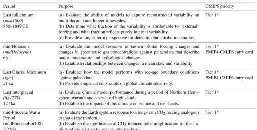
Table 1.Characteristics, purpose, and CMIP6 priority of the five PMIP4-CMIP6 experiments. All experiments can be run independently. Calendar ages are expressed in Common Era (CE) and geological ages are expressed in thousand years (ka) or million years (Ma) before present (BP), with present defined as 1950.
Period Purpose CMIP6 priority
Last millennium (past1000) 850–1849 CE
(a) Evaluate the ability of models to capture reconstructed variability on multi-decadal and longer timescales.
(b) Determine what fraction of the variability is attributable to “external” forcing and what fraction reflects purely internal variability.
(c) Provide a longer-term perspective for detection and attribution studies.
Tier 1*
mid-Holocene (midHolocene) 6 ka
(a) Evaluate the model response to known orbital forcing changes and changes in greenhouse gas concentrations against palaeodata that describe major temperature and hydrological changes.
(b) Establish relationships between changes in mean state and variability
Tier 1*
PMIP4-CMIP6 entry card
Last Glacial Maximum (lgm)
21 ka
(a) Evaluate how the model performs with ice-age boundary conditions against palaeodata.
(b) Provide empirical constraints on global climate sensitivity.
Tier 1*
PMIP4-CMIP6 entry card
Last Interglacial
(lig127k)
127 ka
(a) Evaluate climate model performance during a period of Northern Hemi-sphere warmth and a sea-level high stand.
(b) Establish the impacts of this climate on sea ice and ice sheets.
Tier 1*
mid-Pliocene Warm Period
(midPlioceneEoi400) 3.2 Ma
(a) Evaluate the Earth system response to a long-term CO2forcing analogous to that of the modern.
(b) Establish the significance of CO2-induced polar amplification for the sta-bility of the ice sheets, sea ice, and sea level.
Tier 1*
* It is not mandatory to perform all Tier 1 experiments to take part in PMIP4-CMIP6, but it is mandatory to run at least one of the PMIP4-CMIP6 entry cards.
(land area is expanded relative to present due to the lower sea level, Fig. 2), and lower atmospheric greenhouse gas concen-trations. It is a particularly relevant time period for under-standing near-future climate change because the magnitude of the forcing and temperature response from the LGM to present is comparable to that projected from present to the end of the 21st century (Braconnot et al., 2012).
Evaluation of the PMIP3-CMIP5 MH and LGM ex-periments has demonstrated that climate models simulate changes in the large-scale features that are governed by the energy and water balance reasonably well (Harrison et al., 2014, 2015; Li et al., 2013), including changes in land– sea contrast and high-latitude amplification of temperature changes (Izumi et al., 2013, 2015). These results confirm that the simulated relationships between large-scale patterns of temperature and precipitation change in future projec-tions are credible. However, the PMIP3-CMIP5 simulaprojec-tions of MH and LGM climates show a limited ability to predict reconstructed patterns of climate change overall (Hargreaves et al., 2013; Hargreaves and Annan, 2014; Harrison et al., 2014, 2015). At least in part, this likely arises from persistent problems in simulating regional climates. For example, state-of-the-art models cannot adequately reproduce the northward penetration of the African monsoon in response to the MH orbital forcing (Perez-Sanz et al., 2014; Pausata et al., 2016), which has been noted since PMIP1 (Joussaume et al., 1999).
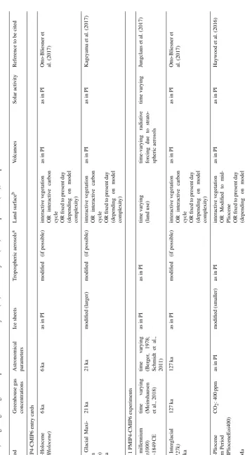
T able 2. Summary of the change in boundary conditions with respect to piContr ol (abbre viated as “PI”) for each PM IP4-CMIP6 experiment. Calendar ages are expressed in Common Era (CE) and geological ages are expressed in thousand years (ka) or million years (Ma) before present (BP), with present defined as 1950. Period Greenhouse g as concentrations Astronomical parameters Ice sheets T ropospheric aerosols a Land surf ace b V olcanoes Solar acti vity Reference to be cited PMIP4-CMIP6 entry cards
mid-Holocene (midHolocene
) 6 ka 6 ka 6 ka as in PI modified (if possible) interacti v e v egetation OR interacti v e carbon cycle OR fix ed to present day (depending on model comple xity) as in PI as in PI Otto-Bliesner et al. (2017) Last Glacial
Maxi-mum (lgm
) 21 ka 21 ka 21 ka modified (lar ger) modified (if possible) interacti v e v egetation OR interacti v e carbon cycle OR fix ed to present day (depending on model comple xity) as in PI as in PI Kage yama et al. (2017) T ier 1 PMIP4-CMIP6 experiments Last millennium ( past1000 ) 850–1849 CE time v arying (Meinshausen et al., 2018) time v arying (Ber ger , 1978; Schmidt et al., 2011) as in PI as in PI time v arying (land use) time-v arying radiati v e forcing due to strato-spheric aerosols time v arying Jungclaus et al. (2017) Last Inter glacial (lig127k) 127 ka 127 ka 127 ka as in PI modified (if possible) interacti v e v egetation OR interacti v e carbon cycle OR fix ed to present day (depending on model comple xity) as in PI as in PI Otto-Bliesner et al. (2017)
mid-Pliocene Warm
[image:5.612.126.476.78.726.2]140 135 130 125 120 115 Age (ka) 5 4 3 -40 0 40 80 180 200 220 240 260 280 300 400 500 600 700 July insolation (65°N) (Wm-2)
Carbon dioxide (ppm)
Methane (ppbv) LIG
(Difference from 1950 CE)
Benthic 18O (‰)
Sea level (m)
-40 0 40 80
1000 1200 1400 1600 1800 2000 Year CE -200 -160 -120 -80 -40 0 40 280 300 320 340 360 380 0 -5 -10 -15 -20 -25 -0.3 -0.2 -0.1 0 0.1 400 800 1200 1600 2000
Sea level (mm)
Volcanic radiative forcing (Wm )-2
Total solar irradiance (Wm )-2
(Differences from 1976–2006 mean) (Difference from 2000 CE)
LM H
3.25 3.2 3.15
Age (Ma) 5 4 3 -40 0 40 80 200 300 400 500 -140 -120 -100 -80 -60 -40 -20 0 20 40 60
(Range or ± 2.0 sd; 3.3–3.0 Ma) MPWP
25 20 15 10 5 0
Age (ka) -40 0 40 80 180 200 220 240 260 280 300 400 500 600 700 -120 -100 -80 -60 -40 -20 0 20 40 60
δ18O (‰) Sea level LGM MH (a) (b) (c) (d) (e) (f) (g) (h) (i)
(j) (k) (l)
(m) (n) (o)
(p)
[image:6.612.62.532.65.416.2](q)
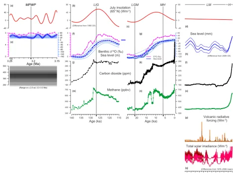
Figure 1.Context of the PMIP4 experiments (from left to right: mPWP, mid-Pliocene Warm Period; LIG, Last Interglacial; LGM, Last
Glacial Maximum; MH, mid-Holocene; LM, last millennium; H, CMIP6 historical simulation):(a–d)insolation anomalies (differences from 1950 CE), for July at 65◦N, calculated using the programs of Laskar et al. (2004, panela) and Berger (1978, panelsb–d);(e)δ18O (magenta, Lisiecki and Raymo, 2005, scale on the left), and sea level (blue line, Rohling et al., 2014; blue shading, a density plot of 11 mid-Pliocene sea-level estimates from Dowsett and Cronin, 1990; Wardlaw and Quinn, 1991; Krantz, 1991; Raymo et al., 2009; Dwyer and Chandler, 2009; Naish and Wilson, 2009; Masson-Delmotte et al., 2013; Rohling et al., 2014; Dowsett et al., 2016. Scale on the right);(f)and(g)
δ18O (magenta, Lisiecki and Raymo, 2005,δ18O scale on the left), and sea level (blue dots, with light-blue 2.5, 25, 75, and 97.5 percentile bootstrap confidence intervals, Spratt and Lisiecki, 2016; blue rectangle, LIG high-stand range, Dutton et al., 2015; dark blue lines, Lambeck et al., 2014, sea-level scale on the right in panelg),(h)sea level (Kopp, et al., 2016, scale on the right);(i)CO2for the interval 3.0–3.3 Ma shown as a density plot of eight mid-Pliocene estimates (Raymo et al., 1996; Stap et al., 2016; Pagani et al., 2010; Seki et al., 2010; Tripati et al., 2009; Bartoli et al., 2011; Seki et al., 2010; Kurschner et al., 1996);(j, k)CO2measurements (Bereiter et al., 2015, scale on the left);
(l)CO2measurements (Schmidt et al., 2011, scale on the right);(m, n)CH4measurements (Loulergue et al., 2008, scale on the left);(o) CH4measurements (Schmidt et al., 2011, scale on the right);(p)volcanic radiative forcing (Schmidt et al., 2012, scale on the right);(q)total solar irradiance (Schmidt et al., 2012, scale on the right).
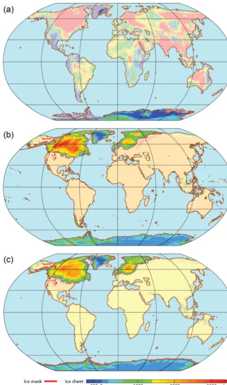
sheets at the Last Glacial Maximum remains. The protocol for the PMIP4-CMIP6lgmsimulations accounts for this un-certainty by permitting modellers to choose between the old PMIP3 ice sheet (Abe-Ouchi et al., 2015) or one of the two new reconstructions: ICE-6G_C (Argus et al., 2014; Peltier et al., 2015) and GLAC-1D (Tarasov et al., 2012; Briggs et al., 2014; Ivanovic et al., 2016). The impact of the ice sheet and dust forcings will specifically be tested in the lgm ex-periments by (i) using different ice sheet reconstructions for
Tier 1simulations (Fig. 2), (ii) performingTier 2dust sensi-tivity experiments (Sect. 3.2.1, Kageyama et al., 2017), and (iii) performingTier 2individual forcing sensitivity experi-ments (Sect. 3.2.2, Kageyama et al., 2017). The inclusion of dust forcing in these simulations is new for PMIP4.
2.2 The last millennium (past1000)
Figure 2.Changes in boundary conditions related to changes in ice sheets for themidPliocene-eoi400(a)andlgm(b: ICE-6G_C andc: GLAC-1D) experiments. Coastlines for the palaeo-period shown as brown contours. Ice sheet boundaries for each period shown as red contours. Bright shading: changes in altitude over regions covered by ice sheets during the considered palaeo-period. Faded shading: changes in altitude over ice-free regions.
2015) period of multi-decadal to multi-centennial changes in climate, with contrasting periods such as the Medieval Cli-mate Anomaly and the Little Ice Age. This interval was char-acterized by variations in solar, volcanic, and orbital forc-ings (Fig. 1), which acted under climatic background con-ditions similar to today. This interval provides a context for analysing earlier anthropogenic impacts (e.g. land-use changes) and the current warming due to increased atmo-spheric greenhouse gas concentrations. It also helps constrain the uncertainty in the future climate response to a sustained anthropogenic forcing.
The PMIP3-CMIP5past1000simulations show relatively good agreement with regional climate reconstructions for the Northern Hemisphere, but less agreement for the Southern Hemisphere. They also provided an assessment of climate variability on decadal and longer scales and information on predictability under forced and unforced condition experi-ments (Fernández-Donado et al., 2013). Single-model en-sembles have provided improved understanding of the im-portance of internal versus forced variability and of the in-dividual forcings when compared to reconstructions at both global and regional scales (Man et al., 2012, 2014; Phipps et al., 2013; Schurer et al., 2014; Man and Zhou, 2014; Otto-Bliesner et al., 2016). Other studies focused on the temper-ature difference between the warmest and coldest centen-nial or multi-centencenten-nial periods and their relationship with changes in external forcing, in particular variations in solar irradiance (e.g. Hind and Moberg, 2013).
The PMIP4-CMIP6past1000simulation (Jungclaus et al., 2017) builds on the DECK experiments, in particular the pre-industrial control (piControl) simulation as an unforced ref-erence, and thehistoricalsimulations (Eyring et al., 2016). Thepast1000simulations provide initial conditions for his-toricalsimulations that can be considered superior to the pi-Controlstate, as they integrate information from the forcing history (e.g. large volcanic eruptions in the early 19th cen-tury). It is therefore mandatory to continue thepast1000 sim-ulations into the historical period when running this simula-tion. The PMIP4-CMIP6past1000protocol uses a new, more comprehensive reconstruction of volcanic forcing (Sigl et al., 2015) and ensures a more continuous transition from the pre-industrial past to the future. The final decisions resulted from strong interactions with the groups producing the different forcing fields for the historical simulations (Jungclaus et al., 2017).
2.3 The Last Interglacial (lig127k)
The Last Interglacial (ca. 130–115 ka before present) was characterized by a Northern Hemisphere insolation seasonal cycle that was even larger than for the mid-Holocene (Otto-Bliesner et al., 2017). This resulted in a strong amplifica-tion of high-latitude temperatures and reduced Arctic sea ice. Global mean sea level was at least 5 m higher than now for at least several thousand years (e.g. Dutton et al., 2015). Both the Greenland and Antarctic ice sheets contributed to this sea-level rise, making it an important period for test-ing our knowledge of climate–ice sheet interactions in warm climates. The availability of quantitative climate reconstruc-tions for the Last Interglacial (e.g. Capron et al., 2014) makes it feasible to evaluate these simulations and assess regional climate changes.
Figure 3.Maps of dust deposition (g m−2a−1)simulated with the Community Earth System Model for the(a)PI (pre-industrial; Albani et al., 2016),(b)MH (mid-Holocene; Albani et al., 2015), and(c)LGM (Last Glacial Maximum; Albani et al., 2014). Maps of dust deposition (g m−2a−1)for the LGM,(d)simulated with the Hadley Centre Global Environment Model 2-Atmosphere (Hopcroft et al., 2015), and reconstructed from a global interpolation of palaeodust data (Lambert et al., 2015).
large differences between simulated and reconstructed mean annual surface temperature anomalies compared to present, particularly for Greenland and the Southern Ocean, and in the temperature trends in transient experiments run for the whole interglacial (Bakker et al., 2013; Lunt et al., 2013). Part of this discrepancy stems from the fact that the climate recon-structions comprised the local maximum interglacial warm-ing, and this was not globally synchronous, an issue which is addressed in the PMIP4-CMIP6 protocol.
The PMIP4-CMIP6 lig127kexperiment will help to de-termine the interactions between a warmer climate (higher atmospheric and oceanic temperatures, changed precipita-tion, and changed surface mass and energy balance) and the ice sheets (specifically, their thermodynamics and dy-namics). The major changes in the experimental proto-col for lig127k, compared to the pre-industrial DECK ex-periment, are changes in the astronomical parameters and greenhouse gas concentrations (Table 2 and Otto-Bliesner et al., 2017). Meaningful analyses of these simulations are now possible because of the concerted effort to synchro-nize the chronologies of individual records and thus pro-vide a spatial–temporal picture of Last Interglacial temper-ature change (Capron et al., 2014, 2017), and also to doc-ument the timing of the Greenland and Antarctic contribu-tions to sea level (Winsor et al., 2012; Steig et al., 2015). Re-gional responses of tropical hydroclimate and polar sea ice to the climate forcing can be assessed and compared to the
mid-Holocene. Outputs from thelig127kexperiment will be used by ISMIP6 to force stand-alone ice sheet experiments (lastIntergacialforcedism) in order to quantify the potential sea-level change associated with this climate.
2.4 The mid-Pliocene Warm Period (midPliocene-eoi400)
al., 2013; Masson-Delmotte et al., 2013). However, as is the case for the Last Interglacial, the PlioMIP simulations were not always performed using the same models that were used in PMIP3-CMIP5.
The PMIP4-CMIP6 midPliocene-eoi400 experiment (Haywood et al., 2016) is designed to elucidate the long-term response of the climate system to a concentration of atmospheric CO2 close to the present one: 400 ppm (long-term climate sensitivity or Earth system sensitivity). It will also be used to assess the response of ocean circu-lation, Arctic sea ice, modes of climate variability (e.g. El Niño–Southern Oscillation), the global hydrological cycle, and regional monsoon systems to elevated concentrations of atmospheric CO2. The simulations have the potential to be informative about which emission reduction scenarios are required to keep the increase in global annual mean temperatures below 2◦C by 2100 CE. Boundary conditions (Table 2) include modifications to global ice distributions (Fig. 2), topography/bathymetry, vegetation, and CO2 and are provided by the US Geological Survey Pliocene Research and Synoptic Mapping Project (PRISM4: Dowsett et al., 2016).
2.5 Palaeoclimatic and palaeoenvironmental data for the PMIP4-CMIP6 periods
The choice of the time periods for the PMIP4-CMIP6 sim-ulations has been made bearing in mind the availability of palaeoenvironmental and/or palaeoclimate reconstructions that can be used for model evaluation and diagnosis. Past en-vironmental and climatic changes are typically documented at specific sites, whether on land, in ocean sediments or in corals, or from ice cores. The evaluation of climate simu-lations such as those conducted for PMIP4-CMIP6 requires these palaeoclimatic and palaeoenvironmental data to be syn-thesized for specific time periods. A major challenge in building such syntheses is to synchronize the chronologies of the different records. There are many syntheses of infor-mation on past climates and environments. Table 3 lists some of the sources of quantitative reconstructions for the PMIP4-CMIP6 time periods, but it is not our goal to provide an ex-tensive review of these resources here.
Much of the information on palaeoclimates comes from the impact of climatic changes on the environment, such as on fires, dust, marine microfauna, and vegetation. Past climatic information is also contained in isotopic ratios of oxygen and carbon, which can be found in ice sheets, speleothems, or the shells of marine organisms. Ocean circu-lation can be documented by geochemical tracers in marine sediments from the sea floor (e.g.114C,δ13C,231Pa/230Th, εNd). The fact that these physical, chemical, or biological in-dicators are indirect records of the state of the climate system and can also be sensitive to other factors (for example, vege-tation is affected by atmospheric CO2concentrations) has to be taken into account in model–data comparisons.
Compar-isons with climate model output can therefore be performed from different points of view: either the climate model output can be directly compared to reconstructions of past climate variables or the response of the climatic indicator itself can be simulated from climate model output and compared to the climate indicator. Such “forward” models include dynami-cal vegetation models, tree ring models, or models comput-ing the growth of foraminifera, for which specific output is needed (cf. Sect. 4.3). Some palaeoclimatic indicators, such as meteoric water isotopes and vegetation, are computed by the climate model as it is running and are also examples of this forward modelling approach. Modelling the impacts of past climate changes on the environment is key to under-standing how climatic signals are transmitted to past climate records. It also provides an opportunity to test the types of models that are used in the assessment of the impacts of fu-ture climate changes on the environment.
3 Analysing the PMIP4-CMIP6 experiments
The community using PMIP simulations is very broad, from climate modellers and palaeoclimatologists to biolo-gists studying recent changes in biodiversity and archaeol-ogists studying potential impacts of past climate changes on human populations. Here, we highlight several topics of anal-yses that will benefit from the new experimental design and from using the full PMIP4-CMIP6 ensemble.
3.1 Comparisons with palaeoclimate and palaeoenvironemental reconstructions, benchmarking, and beyond
Model–data comparisons for each period will be one of the first tasks conducted after completion of these simulations. One new feature common to all periods is that we will make use of the fact that modelling groups must also run the his-toricalexperiment, in addition to thepiControlone. Indeed, existing palaeoclimate reconstructions have used different modern reference states (e.g. climatologies for different time intervals) for their calibration, and this has been shown to have an impact on the magnitude of changes reconstructed from climate indicators (e.g. Hessler et al., 2014). These re-constructed climatic changes were usually compared to sim-ulated climate anomalies w.r.t. a piControl simulation be-cause running thehistoricalsimulations was not systematic in previous phases of PMIP. This prevented investigation of the impact of these reference state assumptions on model– data comparisons. More precisely, understanding the impact of the reference states is important for quantifying the un-certainties in interpretations of climate proxies and hence for evaluating model results.
re-constructions, and thus identify possible model biases or other problems (e.g. Hopcroft and Valdes, 2015a). An en-semble of metrics has already been developed for the PMIP3-CMIP5 midHoloceneandlgmsimulations (e.g. Harrison et al., 2014). Applied to the PMIP4-CMIP6 midHoloceneand lgm “entry card” simulations, these will provide a rigorous assessment of model improvements compared to previous phases of PMIP. Furthermore, for the first time, thanks to the design of the PMIP4-CMIP6 experiments, we will be able to consider the impact of forcing uncertainties on simulated climate in the benchmarking. The benchmarking metrics will also be expanded to other periods and data sets so that sys-tematic biases for different periods and for the present day can be compared. Benchmarking the ensemble of the PMIP4-CMIP6 simulations for all the periods will therefore allow quantification of the climate-state dependence of the model biases, a topic which is highly relevant for a better assess-ment of potential biases in the projected climates in CMIP6. In addition, it will be possible to analyse the potential re-lationships between model biases in different regions and/or in different variables (such as temperature vs. hydrological cycle) across the PMIP ensemble, as well as for the recent climate. One further objective for the PMIP4-CMIP6 bench-marking will be to develop more process-oriented metrics, making use of the fact that palaeoclimatic data document different aspects of climate change. There are many aspects of the climate system that are difficult to measure directly, and which are therefore difficult to evaluate using traditional methods. The “emergent constraint” (e.g. Sherwood et al., 2014) concept, which is based on identifying a relationship with a more easily measurable variable, has been success-fully used by the carbon-cycle and modern climate commu-nities and holds great potential for the analysis of palaeo-climate simulations. Using multiple time periods to examine “emergent” constraints will ensure that they are robust across climate states.
3.2 Analysing the response of the climate system to multiple forcings
Multi-period analyses provide a way of determining whether systematic model biases affect the overall response and the strength of feedbacks independently of climate state. One challenge will be to develop new approaches to analyse the PMIP4-CMIP6 ensemble so as to separate the impacts of model structure (including choice of resolution, parameteri-zations, and complexity) on the simulated climate. Similarly, the uncertainties in boundary conditions will be addressed for periods with proposed alternative forcings.
Quantifying the role of forcings and feedbacks in creating climates different from today has been a focus of PMIP for many years. Many CMIP6 models will include representa-tions of new forcings, such as dust, or improved represen-tations of major radiative feedback processes, such as those related to clouds. This will allow a broader analysis of
feed-backs than was possible in PMIP3-CMIP5. We will evalu-ate the impact of these new processes and improved realiza-tions of key forcings on climates at global, large (e.g. polar amplification, land–sea contrast), as well as regional scales, together with the mechanisms explaining these impacts. A particular emphasis will be put on the modulation of the cli-mate response to a given forcing by the background clicli-mate state and how it affects changes in cloud feedbacks, snow and ice sheets (such as in e.g. Yoshimori et al., 2011), vegetation, and ocean deep water formation. Identification of similarities between past climates and future climate projections such as that found for land–sea contrast or polar amplification (Izumi et al., 2013, 2015; Masson-Delmotte et al., 2006), or for snow and cloud feedbacks for particular seasons (Braconnot and Kageyama, 2015), will be used to provide better understand-ing of the relationships between patterns and timescales of external forcings and patterns and timing of the climate re-sponses.
These analyses should provide new constraints on climate sensitivity. Previous attempts that used information about the LGM period have been hampered by the fact that there were too fewlgmexperiments to draw statistically robust conclu-sions (Crucifix et al., 2006; Hargreaves et al., 2012; Harrison et al., 2014; Hopcroft and Valdes, 2015b). These attempts also ignored uncertainties in forcings and boundary condi-tions. PMIP4-CMIP6 is expected to result in a much larger ensemble oflgmexperiments. The issue of climate sensitiv-ity and Earth system sensitivsensitiv-ity (PALEOSENS Project Mem-bers, 2012) will also be examined through joint analysis of multiple palaeoclimate simulations and climate reconstruc-tions from different archives.
The PMIP4-CMIP6 ensemble will allow new analyses of the impact of smaller (mPWP) or larger (LGM) ice sheets. The ocean and sea ice feedbacks will also be analysed. The representation of sea ice and Southern Ocean circula-tion proved to be problematic in previous simulacircula-tions of colder (LGM, Roche et al., 2012) and warmer climates (LIG, Bakker et al., 2013; Lunt et al., 2013) and we are eager to analyse improved models for this area which is key for atmosphere–ocean carbon exchanges. For the LGM, there is evidence of a shallower and yet active overturning circulation in the North Atlantic (e.g. Lynch-Stieglitz et al., 2007; Böhm et al., 2015). Understanding this oceanic circulation for the LGM and the other PMIP4 periods, as well as its links to sur-face climate, is a topic of high importance since the Atlantic Meridional Overturning Circulation could modulate future climate changes at least in regions around the North Atlantic. The PMIP4 multi-period ensemble, for which we require im-proved simulations in terms of spin-up, will strengthen the analyses for this particular topic compared to previous phases of PMIP (Marzocchi and Jansen, 2017).
forcings should provide a better understanding of changes in ENSO behaviour (Zheng et al., 2008; An and Choi, 2014) and help determine whether state-of-the-art climate models underestimate low-frequency variability (Laepple and Huy-bers, 2014). Analyses will focus on how models reproduce the relationship between changes in seasonality and interan-nual variability (Emile-Geay et al., 2016), the diversity of El Niño events (Capotondi et al., 2015; Karamperidou et al., 2015; Luan et al., 2015), and the stability of teleconnections within the climate system (e.g. Gallant et al., 2013; Batehup et al., 2015).
3.3 Interactions with other CMIP6 MIPs and the WCRP Grand Challenges
PMIP has already developed strong links with several other CMIP6 MIPs (Table 4). CFMIP includes an idealized experi-ment that allows the investigation of cloud feedbacks and as-sociated circulation changes in a colder versus warmer world. This will assist in disentangling the processes at work in the PMIP4 simulations. We have also required CFMIP-specific output to be implemented in the PMIP4-CMIP6 simulations so that the same analyses can be carried out for both the PMIP4 and CFMIP simulations. This will ensure that the simulated cloud feedbacks in different past and future cli-mates can be directly compared.
Interactions between PMIP and other CMIP6 MIPs have mutual benefits: PMIP provides (i) simulations of large cli-mate changes that have occurred in the past and (ii) evalua-tion tools that capitalize on extensive data syntheses, while other MIPs will employ diagnostics and analyses that will be useful for analysing the PMIP4 experiments. We are ea-ger to settle collaborations with the CMIP6 MIPs listed in Table 4 and have ensured that all the outputs necessary for the application of common diagnostics between PMIP and these MIPs will be available (see Sect. 4.3). Links with CFMIP and ISMIP6 mean that PMIP will contribute to the World Climate Research Programme (WCRP) Grand Chal-lenges on “Clouds, Circulation and Climate Sensitivity” and “Cryosphere and Sea Level” respectively. PMIP will provide input to the WCRP Grand Challenge on “Regional Climate Information”, through a focus on evaluating the mechanisms of regional climate change in the past.
4 Model configuration, experimental set-up, documentation, and required output.
To achieve the PMIP4 goals and benefit from other simula-tions in CMIP6, particular care must be taken with model versions and the implementation of the experimental proto-cols. Here we summarize the guidelines that are common to all the experiments, focusing on the requirements to ensure strict consistency between CMIP6 and PMIP4 experiments. These concern model complexity, forcings, and mineral dust,
which is a new feature in the PMIP4 experiments. This sec-tion also provides guidelines for the documentasec-tion and re-quired output. The reader is referred to the PMIP4 compan-ion papers on the specific periods for details of the set-up of each PMIP4-CMIP6 experiment.
4.1 Model version, set-up, and common design of all PMIP4-CMIP6 experiments
The climate models taking part in CMIP6 are very diverse: some represent solely the physics of the climate system, some include the carbon cycle and other biogeochemical cy-cles, and some include interactive natural vegetation and/or interactive dust cycle/aerosols. It is mandatory that the model version used for the PMIP4-CMIP6 experiments is exactly the same as for the DECK andhistorical simulations. It is highly preferable that it is also exactly the same as for any other CMIP6 experiments, for ease and robustness of com-parison between the MIPs. The experimental set-up for each simulation is based on the DECK pre-industrial control ( pi-Control) experiment (Eyring et al., 2016), i.e. thepiControl forcings and boundary conditions are modified to obtain the forcings and boundary conditions necessary for each PMIP4-CMIP6 palaeoclimate experiment (Table 2). No additional interactive component should be included in the model un-less it is already included in the DECK version. Such changes would prevent rigorous analyses of the responses to forc-ings across multiple time periods or between MIPs (Sect. 3) because the differences between the experiments could then arise from both the models’ characteristics and the response to changes in external forcings. Adding an interactive com-ponent usually affects the piControl simulation as well as simulations of past climates (Braconnot et al., 2007), so it is very important that experiments for PMIP4-CMIP6 and DECK are run with exactly the same model version.
Table 3.Examples of data syntheses for the PMIP4-CMIP6 periods. MAT: mean annual temperature; MAP: mean annual precipitation;α: ratio of the actual evaporation over potential evaporation; MTCO: mean temperature of the coldest month; MTWA: mean temperature of the warmest month; SST: sea-surface temperature.
Reference Variables Time period Comments Data available from
Mann et al. (2009) MAT 500–2006 CE Gridded data set (5◦) http://science.sciencemag.org/content/suppl/ 2009/11/25/326.5957.1256.DC1
PAGES 2k Consor-tium (2013)
MAT past 2000 years Individual sites;
Arctic data updated 2014
https://www.ncdc.noaa.gov/paleo-search/ study/12621
Bartlein et al. (2011) MAT, MAP,
α, MTCO,
MTWA
6000±500 yr; 21 000±1000 yr
Gridded data set (2◦) https://www.ncdc.noaa.gov/paleo/study/9897
MARGO Project
Members (2009)
Mean
an-nual, winter, summer SST
21000±2000 yr Gridded data set (5◦) http://www.ncdc.noaa.gov/paleo/study/ 12034
http://doi.pangaea.de/10.1594/PANGAEA. 733406
Turney and Jones (2010)
MAT, SST Maximum warmth
during LIG
Individual sites (100 terrestrial; 162 ma-rine)
http://onlinelibrary.wiley.com/store/ 10.1002/jqs.1423/asset/supinfo/JQS_ 1423_sm_suppInfo.pdf?v=1&s=
1726938c44b8762e15aaf17514fc076c855b8ed1
Capron et al. (2014, 2017)
MAT,
sum-mer SST
114–116, 119–121, 124–126, 126–128, 129–131 ka
47 high-latitude sites https://doi.org/10.1594/PANGAEA.841672
Dowsett et al. (2012) SST 3.264–3.025 Ma Further information available in Dowsett et al. (2016)
http://www.nature.com/nclimate/ journal/v2/n5/full/nclimate1455.html# supplementary-information
Salzmann et al. (2013)
MAT 3.3–3.0 Ma http://www.nature.com/nclimate/journal/v3/
n11/extref/nclimate2008-s1.pdf
Two experiments, lgm and midPliocene-eoi400, require modified ice sheets (Fig. 2), which also implies consistent modification of the coastlines, ocean bathymetry (if feasi-ble for midPliocene-eoi400), topography, and land surface types over the continents, and to ensure that rivers reach the ocean in order to close the global freshwater budget. The ini-tial global mean ocean salinity should be adjusted for these ice volume changes and modelling groups are advised to en-sure that the total mass of the atmosphere remains the same in all experiments.
For each experiment, the greenhouse gases and astronom-ical parameters should be modified from the DECK piCon-trolexperiment (Table 2). Spin-up procedures will differ ac-cording to the model and type of simulation, but the spin-up should be long enough to avoid significant drift in the anal-ysed data. Initial conditions for the spin-up can be taken from an existing simulation. The model should be run until the ab-solute value of the trend in global mean sea-surface temper-ature is less than 0.05 K per century and the Atlantic Merid-ional Overturning Circulation is stable. A parallel require-ment for carbon-cycle models and/or models with dynamic
vegetation is that the 100-year mean global carbon uptake or release by the biosphere is<0.01 Pg C yr−1.
4.2 A new feature of the PMIP simulations: mineral dust
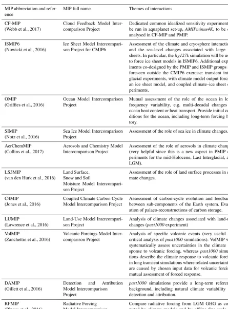
advis-Table 4.Interactions of PMIP and other CMIP6 MIPs.
MIP abbreviation and refer-ence
MIP full name Themes of interactions
CF-MIP
(Webb et al., 2017)
Cloud Feedback Model Inter-comparison Project
Dedicated common idealized sensitivity experiment to be run in aquaplanet set-up,AMIPminus4K, to be co-analysed in CF-MIP and PMIP.
ISMIP6
(Nowicki et al., 2016)
Ice Sheet Model Intercompari-son Project for CMIP6
Assessment of the climate and cryosphere interactions and the sea-level changes associated with large ice sheets. In particular, thelig127ksimulation will be used to force ice sheet models in ISMIP6. Additional exper-iments co-designed by the PMIP and ISMIP groups are foreseen outside the CMIP6 exercise: transient inter-glacial experiments, with climate model output forcing an ice sheet model, and coupled climate–ice sheet ex-periments.
OMIP
(Griffies et al., 2016)
Ocean Model Intercomparison Project
Mutual assessment of the role of the ocean in low-frequency variability, e.g. multi-decadal changes in ocean heat content or heat transport. Provide initial con-ditions for the ocean, including long-term forcing his-tory.
SIMIP
(Notz et al., 2016)
Sea Ice Model Intercomparison Project
Assessment of the role of sea ice in climate changes.
AerChemMIP (Collins et al., 2017)
Aerosols and Chemistry Model Intercomparison Project
Assessment of the role of aerosols in climate changes (very helpful since this is a new aspect in PMIP ex-periments for the mid-Holocene, Last Interglacial, and LGM).
LS3MIP
(van den Hurk et al., 2016)
Land Surface, Snow and Soil
Moisture Model Intercompari-son Project
Assessment of the role of land surface processes in cli-mate changes.
C4MIP
(Jones et al., 2016)
Coupled Climate Carbon Cycle Model Intercomparison Project
Assessment of carbon-cycle evolution and feedbacks between sub-components of the Earth system. Evalu-ation of palaeo-reconstructions of carbon storage.
LUMIP
(Lawrence et al., 2016)
Land-Use Model Intercompari-son Project
Analysis of climate changes associated with land-use changes (past1000experiment)
VolMIP
(Zanchettin et al., 2016)
Volcanic Forcings Model Inter-comparison Project
Analysis of specific volcanic events (very useful for critical analysis ofpast1000simulations). VolMIP will systematically assess uncertainties in the climate re-sponse to volcanic forcing, whereaspast1000 simula-tions describe the climate response to volcanic forcing in long transient simulations where related uncertainties are caused by chosen input data for volcanic forcing: mutual assessment of forced response.
DAMIP
(Gillett et al., 2016)
Detection and Attribution Model Intercomparison Project
past1000 simulations provide a long-term reference background, including natural climate variability for detection and attribution.
RFMIP
(Pincus et al., 2016)
Radiative Forcing Model Intercomparison Project
[image:13.612.73.519.96.699.2]able to test the atmosphere model behaviour before running the fully coupledlgmsimulation.
To allow experiments with prescribed dust changes, three-dimensional monthly climatologies of dust atmospheric mass concentrations are provided for thepiControl,midHolocene, andlgm. These are based on two different models (Albani et al., 2014, 2015, 2016; Hopcroft et al., 2015, Fig. 3) and modelling groups are free to choose between these data sets. Additional dust-related fields (dust emission flux, dust load, dust aerosol optical thickness, short- and long-wave radia-tion, surface and top of the atmosphere dust radiative forc-ing) are also available from these simulations. Implementa-tion should follow the same procedure as for the historical experiment. The implementation for thelig127kexperiment should use the same data set as for the midHolocene one. Since dust plays an important role in ocean biogeochem-istry (e.g. Kohfeld et al., 2005), three dust maps are pro-vided for the lgm experiment. Two of these are consistent with the climatologies of dust atmospheric mass concentra-tions; the other is primarily derived from palaeoenvironmen-tal observations (Lambert et al., 2015, Fig. 3). The modelling groups should use consistent data sets for the atmosphere and the ocean biogeochemistry. The Lambert et al. (2015) data set can therefore be used for models that cannot include the changes in atmospheric dust according to the other two data sets.
4.3 Documentation and required model output for the PMIP4-CMIP6 database
Detailed documentation of the PMIP4-CMIP6 simulations is required. This should include
– a description of the model and its components;
– information about the boundary conditions used, partic-ularly when alternatives are allowed;
– information on the implementation of boundary condi-tions and forcings. Figures showing the land–sea mask, land–ice mask, and topography as implemented in a given model are useful for the lgm and midPliocene-eoi400 experiments, while figures showing insolation are particularly important for the midHolocene and lig127kexperiments. Checklists for the implementation of simulations are provided in the PMIP4 papers, which give detailed information for each experiment; and – information about the initial conditions and spin-up
technique used. A measure of the changes in key vari-ables (Table 5) should be provided in order to assess remaining drift.
Documentation should be provided via the ESDOC website and tools provided by CMIP6 (http://es-doc.org/) to facilitate communication with other CMIP6 MIPs. This documenta-tion should also be provided for the PMIP4 website to
facili-tate linkages with non-CMIP6 simulations. The PMIP4 spe-cial issue, shared betweenGeoscientific Model Development andClimate of the Past, provides a further opportunity for modelling groups to document specific aspects of their sim-ulations. We also require the groups to document the spin-up phase of the simulations by saving a limited set of variables during this phase (Table 5).
The data stored in the CMIP6 database should be repre-sentative of the equilibrium climates of the MH, LGM, LIG, and mPWP periods, and of the transient evolution of climate between 850 and 1849 CE for thepast1000simulations. A minimum of 100 years’ output is required for the equilibrium simulations but, given the increasing interest in analysing multi-decadal variability (e.g. Wittenberg, 2009), modelling groups are encouraged to provide outputs for 500 years or more if possible. Daily values should also be provided and will allow the calendar issue to be accounted for (see Ap-pendix). The list of variables required to analyse the PMIP4-CMIP6 palaeoclimate experiments (https://wiki.lsce.ipsl.fr/ pmip3/doku.php/pmip3:wg:db:cmip6request) reflects plans for multi-time period analyses and for interactions with other CMIP6 MIPs. We have included relevant variables from the data requests of other MIPs, including the CFMIP-specific diagnostics on cloud forcing, as well as land surface, snow, ocean, sea ice, aerosol, carbon cycle, and ice sheet variables from LS3MIP, OMIP, SIMIP, AerChemMIP, C4MIP, and IS-MIP6 respectively. Some of these variables are also required to diagnose how climate signals are recorded by palaeocli-matic sensors via models of tree growth (Li et al., 2014), veg-etation dynamics (Prentice et al., 2011), or marine planktonic foraminifera (e.g. Lombard et al., 2011; Kageyama et al., 2013), for example. The only set of variables defined specif-ically for PMIP are those describing oxygen isotopes in the climate system. Isotopes are widely used for palaeoclimatic reconstruction and are explicitly simulated in several models. We have asked that mean annual cycles of key variables are included in the PMIP4-CMIP6 data request for equilibrium simulations, as these proved exceptionally useful for analy-ses in PMIP3-CMIP5.
5 Conclusions
The PMIP4-CMIP6 simulations provide a framework to compare current and future anthropogenic climate change with past natural variations of the Earth’s climate. PMIP4-CMIP6 is a unique opportunity to simulate past climates with exactly the same models as are used for simulations of the future. This approach is only valid if the model versions and implementation of boundary conditions are consistent for all periods, and if these boundary conditions are seamless for overlapping periods.
Table 5.Variables to be saved for the documentation of the spin-up phase of the models.
Atmospheric variables top of atmosphere energy budget (global and annual mean)
surface energy budget (global and annual mean)
northern surface air temperature (annual mean over the Northern Hemisphere) southern surface air temperature (annual mean over the Southern Hemisphere)
Oceanic variables Sea-surface temperatures (global and annual mean)
deep ocean temperatures (global and annual mean over depths below 2500 m) deep ocean salinity (global and annual mean over depths below 2500 m)
Atlantic Meridional Overturning Circulation (maximum overturning strength between 0 and 80◦N and below 500 m in depth)
Sea ice variables northern sea ice (annual mean over the Northern Hemisphere) southern sea ice (annual mean over the Southern Hemisphere)
Carbon-cycle variables Global carbon budget
amip
Historical CMIP6 entry card
PMIP4-CMIP6 entry card
midHolocene or lgm abrupt4xCO2
piControl
1pctCO2
PMIP4
past1000
lastInterglacial
midPlioceneEoi400
Quaternary Interglacials Deglaciation lgm sensitivity experiments
plioMIP
pre-Pliocene climates
Isotope modelling DECK
PMIP4-CMIP6 CMIP6
PMIP4-MIPs
and other CMIP6 MIPs VolMIP
CFMIP
AerChemMIP
ISMIP
LS3MIP
C4MIP
DAMIP
OMIP
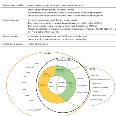
Figure 4.The PMIP4-CMIP6 experiments in the framework of CMIP6(a), with associated MIPs; and in the framework of PMIP4, with its
working groups(b).
climatic periods well documented by palaeoclimatic and palaeoenvironmental records, with climate and environmen-tal changes relevant for the study and projections of future climate changes: the millennium prior to the industrial epoch (past1000), 6000 years ago (midHolocene), the Last Glacial Maximum (lgm), the Last Interglacial (lig127k), and the mid-Pliocene Warm Period (midPliocene-eoi400).
The PMIP4-CMIP6 experiments will also constitute ref-erence simulations for projects developed in the broader PMIP4 initiative. The corresponding sensitivity experiments, or additional experiments, are embedded in the PMIP4 project and are described in the companion papers to this
relate to the CMIP6 DECK and some other CMIP6 MIPs. PMIP4-CMIP6 experiments have been designed to be anal-ysed by both communities.
The PMIP community anticipates major benefits from analysis techniques developed by the other CMIP6 MIPs, in particular in terms of learning about the processes of past cli-mate changes in response to forcings (e.g. greenhouse gases, astronomical parameters, ice sheet and sea-level changes) as well as the role of feedbacks (e.g. clouds, ocean, sea ice). PMIP4-CMIP6 has the potential to be mutually beneficial for the palaeoclimate and present/future climate scientists to learn about natural large climate changes and the mech-anisms at work in the climate system for climate states that are different from today, as future climate is projected to be.
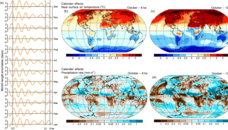
Appendix A: Justification of the requirement to save high-frequency output (daily and 6-hourly)
Figure A1.The calendar effect:(a)month-length anomalies, 140 ka to present, with the PMIP4 experiment times indicated by vertical lines. The month-length anomalies were calculated using the formulation in Kutzbach and Gallimore (1988).(b, c)The calendar effect on October temperature at 6 and 127 ka, calculated using Climate Forecast System Reanalysis near-surface air temperature (https://www.earthsystemcog. org/projects/obs4mips/), 1981–2010 long-term means, and assuming the long-term mean differences in temperature are zero everywhere.
(e, f) The calendar effect on October precipitation at 6 and 127 ka, calculated using the CPC Merged Analysis of Precipitation (CMAP)
Author contributions. MK, PB, and SH organized the main text. The text for each period was initially provided by the leaders of the companion papers, who collated and summarized the contribution of their groups: JJ for the last millennium, BOB for the interglacials, MK for the Last Glacial Maximum, and AH for the mid-Pliocene Warm Period. All authors agreed on the experimental design and contributed text on the background, forcing data sets, or topics in the analysis plan. In addition, the consistency of the forcing data sets for all periods was carefully checked by the contributors of the data sets. The Appendix was written and illustrated by PJB. The final text was refined by RI.
Competing interests. The authors declare that they have no conflict of interest.
Acknowledgements. Masa Kageyama and Qiong Zhang
ac-knowledge funding from French–Swedish project GIWA. Pascale Braconnot, Johann Jungclaus, and Sandy P. Harrison acknowl-edge funding from JPI-Belmont project “PAleao-Constraints on Monsoon Evolution and Dynamics (PACMEDY)” through their respective national funding agencies. Sandy P. Harrison also acknowledges funding from the Australian Research Council (DP1201100343) and from the European Research Council for “GC2.0: Unlocking the past for a clearer future”. Alan M. Hay-wood and Aisling Dolan acknowledge funding from the European Research Council under the European Union’s Seventh Framework Programme (FP7/2007–2013)/ERC grant agreement no. 278636 and the EPSRC-supported Past Earth Network. Ruza F. Ivanovic is funded by a NERC Independent Research Fellowship (no. NE/K008536/1). Steven J. Phipps’s contribution is supported under the Australian Research Council’s Special Research Initiative for the Antarctic Gateway Partnership (project ID SR140300001). Fabrice Lambert acknowledges support from CONICYT projects 15110009, 1151427, ACT1410, and NC120066.
Edited by: Julia Hargreaves
Reviewed by: Steven Sherwood and three anonymous referees
References
Abe-Ouchi, A., Saito, F., Kageyama, M., Braconnot, P., Harrison, S. P., Lambeck, K., Otto-Bliesner, B. L., Peltier, W. R., Tarasov, L., Peterschmitt, J.-Y., and Takahashi, K.: Ice-sheet configuration in the CMIP5/PMIP3 Last Glacial Maximum experiments, Geosci. Model Dev., 8, 3621–3637, https://doi.org/10.5194/gmd-8-3621-2015, 2015.
Albani, S., Mahowald, N. M., Perry, A. T., Scanza, R. A., Zen-der, C. S., Heavens, N. G., Maggi, V., Kok, J. F., and Otto-Bliesner, B. L.: Improved representation of dust size and op-tics in the CESM, J. Adv. Model. Earth Sy., 6, 541–570, https://doi.org/10.1002/2013MS000279, 2014.
Albani, S., Mahowald, N. M., Winckler, G., Anderson, R. F., Bradt-miller, L. I., Delmonte, B., François, R., Goman, M., Heavens, N. G., Hesse, P. P., Hovan, S. A., Kang, S. G., Kohfeld, K. E., Lu, H., Maggi, V., Mason, J. A., Mayewski, P. A., McGee, D., Miao, X., Otto-Bliesner, B. L., Perry, A. T., Pourmand, A., Roberts, H. M.,
Rosenbloom, N., Stevens, T., and Sun, J.: Twelve thousand years of dust: the Holocene global dust cycle constrained by natural archives, Clim. Past, 11, 869–903, https://doi.org/10.5194/cp-11-869-2015, 2015.
Albani, S., Mahowald, N. M., Murphy, L. N., Raiswell, R., Moore, J. K., Anderson, R. F., McGee, D., Bradtmiller, L. I., Del-monte, B., Hesse, P. P., and Mayewski, P. A.: Paleodust vari-ability since the Last Glacial Maximum and implications for iron inputs to the ocean, Geophys. Res. Lett., 43, 3944–3954, https://doi.org/10.1002/2016GL067911, 2016.
An, S.-I. and Choi, J.: Mid-Holocene tropical Pacific climate state, annual cycle, and ENSO in PMIP2 and PMIP3, Clim. Dynam., 43, 957–970, https://doi.org/10.1007/s00382-013-1880-z, 2014. Argus, D. F., Peltier, W. R., Drummond, R., and Moore, A. W.: The
Antarctica component of postglacial rebound model ICE-6G_C (VM5a) based on GPS positioning, exposure age dating of ice thicknesses, and relative sea level histories, Geophys. J. Int., 98, 537–563, https://doi.org/10.1093/gji/ggu140, 2014.
Bakker, P., Stone, E. J., Charbit, S., Gröger, M., Krebs-Kanzow, U., Ritz, S. P., Varma, V., Khon, V., Lunt, D. J., Mikolajewicz, U., Prange, M., Renssen, H., Schneider, B., and Schulz, M.: Last interglacial temperature evolution – a model inter-comparison, Clim. Past, 9, 605–619, https://doi.org/10.5194/cp-9-605-2013, 2013.
Bartlein, P. J. and Shafer, S. L.: The impact of the “calendar effect” and pseudo-daily interpolation algorithms on paleoclimatic data-model comparisons, available at: https://agu.confex.com/agu/ fm16/meetingapp.cgi/Paper/187186 (last access: 6 March 2018), 2016.
Bartlein, P. J., Harrison, S. P., Brewer, S., Connor, S., Davis, B. A. S., Gajewski, K., Guiot, J., Harrison-Prentice, T. I., Hender-son, A., Peyron, O., Prentice, I. C., Scholze, M., Seppä, H., Shu-man, B., Sugita, S., Thompson, R. S., Viau, A., Williams, J., and Wu, H.: Pollen-based continental climate reconstructions at 6 and 21 ka: a global synthesis, Clim. Dynam., 37, 775–802, 2011. Bartoli, G., Honisch, B., and Zeebe, R. E.: Atmospheric
CO2 decline during the Pliocene intensification of North-ern Hemisphere glaciations, Paleoceanography, 26, PA4213, https://doi.org/10.1029/2010PA002055, 2011.
Batehup, R., McGregor, S., and Gallant, A. J. E.: The influence of non-stationary teleconnections on palaeoclimate reconstructions of ENSO variance using a pseudoproxy framework, Clim. Past, 11, 1733–1749, https://doi.org/10.5194/cp-11-1733-2015, 2015. Bereiter, B., Eggleston, S., Schmitt, J., Nehrbass-Ahles, C., Stocker, T. F., Fischer, H., Kipfstuhl, S., and Chappellaz, J.: Revision of the EPICA Dome C CO2 record from 800 to 600 kyr before present, Geophys. Res. Lett., 42, 2014GL061957, https://doi.org/10.1002/2014GL061957, 2015.
Berger, A.: Long-term variations of daily insolation and quaternary climatic changes, J. Atmos. Sci., 35, 2362–2367, 1978. Böhm, E., Lippold, J., Gutjahr, M., Frank, M., Blaser, P., Antz,
B., Fohlmeister, J., Frank, N., Andersen, M. B., and Deininger, M.: Strong and deep Atlantic meridional overturning cir-culation during the last glacial cycle, Nature, 517, 73–76, https://doi.org/10.1038/nature14059, 2015.
Braconnot, P., Otto-Bliesner, B., Harrison, S., Joussaume, S., Pe-terchmitt, J.-Y., Abe-Ouchi, A., Crucifix, M., Driesschaert, E., Fichefet, Th., Hewitt, C. D., Kageyama, M., Kitoh, A., Loutre, M.-F., Marti, O., Merkel, U., Ramstein, G., Valdes, P., Weber, L., Yu, Y., and Zhao, Y.: Results of PMIP2 coupled simula-tions of the Mid-Holocene and Last Glacial Maximum – Part 2: feedbacks with emphasis on the location of the ITCZ and mid- and high latitudes heat budget, Clim. Past, 3, 279–296, https://doi.org/10.5194/cp-3-279-2007, 2007.
Braconnot, P., Harrison, S. P., Kageyama, M., Bartlein, P. J., Masson-Delmotte, V., Abe-Ouchi, A., Otto-Bliesner, B., and Zhao, Y.: Evaluation of climate models using palaeoclimatic data, Nat. Clim. Change, 2, 417–424, 2012.
Briggs, R. D., Pollard, D., and Tarasov, L.: A data-constrained large ensemble analysis of Antarctic evolu-tion since the Eemian, Quaternary Sci. Rev., 103, 91–115, https://doi.org/10.1016/j.quascirev.2014.09.003, 2014.
Caballero, R. and Huber, M.: Spontaneous transition to superrota-tion in warm climates simulated by CAM3, Geophys. Res. Lett., 37, L11701, https://doi.org/10.1029/2010GL043468, 2010. Capotondi, A., Wittenberg, A. T., Newman, M., Di Lorenzo, E., Yu,
J.-Y., Braconnot, P., Cole, J., Dewitte, B., Giese, B., Guilyardi, E., Jin, F.-F., Karnauskas, K., Kirtman, B., Lee, T., Schneider, N., Xue, Y., and Yeh, S.-W.: Understanding ENSO Diversity, B. Am. Meteorol. Soc., 96, 921–938, https://doi.org/10.1175/Bams-D-13-00117.1, 2015.
Capron, E., Govin, A., Stone, E. J., Masson-Delmotte, V., Mulitza, S., Otto-Bliesner, B., Rasmussen, T. L., Sime, L. C., Waelbroeck, C., and Wolff, E. W.: Temporal and spatial structure of multi-millennial temperature changes at high latitudes during the Last Interglacial, Quaternary Sci. Rev., 103, 116–133, 2014. Capron, E., Govin, A., Feng, R., Otto-Bliesner, B., and Wolff,
E. W.: Critical evaluation of climate syntheses to bench-mark CMIP6/PMIP4 127 ka Last Interglacial simulations in the high-latitude regions, Quaternary Sci. Rev., 168, 137–150, https://doi.org/10.1016/j.quascirev.2017.04.019, 2017.
Chen, G.-S., Kutzbach, J. E., Gallimore, R., and Liu, Z.: Calendar effect on phase study in paleoclimate transient simulation with orbital forcing, Clim. Dynam., 37, 1949–1960, 2011.
Collins, W. J., Lamarque, J.-F., Schulz, M., Boucher, O., Eyring, V., Hegglin, M. I., Maycock, A., Myhre, G., Prather, M., Shindell, D., and Smith, S. J.: AerChemMIP: quantifying the effects of chemistry and aerosols in CMIP6, Geosci. Model Dev., 10, 585– 607, https://doi.org/10.5194/gmd-10-585-2017, 2017.
Crucifix, M.: Does the Last Glacial Maximum constrain climate sensitivity?, Geophys. Res. Lett., 33, L18701, https://doi.org/10.1029/2006GL027137, 2006.
Dowsett, H. J. and Cronin, T. M.: High eustatic sea level during the middle Pliocene: Evidence from the southeastern U.S. Atlantic Coastal Plain, Geology, 18, 435–438, 1990.
Dowsett, H. J., Robinson, M. M., Haywood, A. M., Hill, D. J., Dolan, A. M., Stoll, D. K., Chan, W.-L., Abe-Ouchi, A., Chan-dler, M. A., and Rosenbloom, N. A.: Assessing confidence in Pliocene sea surface temperatures to evaluate predictive models, Nat. Clim. Change, 2, 365–371, 2012.
Dowsett, H., Dolan, A., Rowley, D., Moucha, R., Forte, A. M., Mitrovica, J. X., Pound, M., Salzmann, U., Robinson, M., Chan-dler, M., Foley, K., and Haywood, A.: The PRISM4
(mid-Piacenzian) paleoenvironmental reconstruction, Clim. Past, 12, 1519–1538, https://doi.org/10.5194/cp-12-1519-2016, 2016. Dutton, A., Carlson, A. E., Long, A. J., Milne, G. A.,
Clark, P. U., DeConto, R., Horton, B. P., Rahmstorf, S., and Raymo, M. E.: Sea-level rise due to polar ice-sheet mass loss during past warm periods, Science, 349, aaa4019, https://doi.org/10.1126/science.aaa4019, 2015.
Dwyer, G. S. and Chandler, M. A.: Mid-Pliocene sea level and con-tinental ice volume based on coupled benthic Mg/Ca palaeotem-peratures and oxygen isotopes, Philos. T. Roy. Soc. A, 367, 157– 168, 2009.
Emile-Geay, J., Cobb, K. M., Carré, M., Braconnot, P., Leloup, J., Zhou, Y., Harrison, S. P., Corrège, T., McGregor, H. V., Collins, M., Driscoll, R., Elliot, M., Schneider, B., and Tudhope, A.: Links between tropical Pacific seasonal, interannual and or-bital variability during the Holocene, Nat. Geosci., 9, 168–173, https://doi.org/10.1038/ngeo2608, 2016.
Epstein, E. S.: On obtaining daily climatological values from monthly means, J. Climate, 4, 365–368, 1991.
Eyring, V., Bony, S., Meehl, G. A., Senior, C. A., Stevens, B., Stouffer, R. J., and Taylor, K. E.: Overview of the Coupled Model Intercomparison Project Phase 6 (CMIP6) experimen-tal design and organization, Geosci. Model Dev., 9, 1937–1958, https://doi.org/10.5194/gmd-9-1937-2016, 2016.
Fernández-Donado, L., González-Rouco, J. F., Raible, C. C., Am-mann, C. M., Barriopedro, D., García-Bustamante, E., Jungclaus, J. H., Lorenz, S. J., Luterbacher, J., Phipps, S. J., Servonnat, J., Swingedouw, D., Tett, S. F. B., Wagner, S., Yiou, P., and Zorita, E.: Large-scale temperature response to external forcing in simu-lations and reconstructions of the last millennium, Clim. Past, 9, 393–421, https://doi.org/10.5194/cp-9-393-2013, 2013. Flato, G., Marotzke, J., Abiodun, B., Braconnot, P., Chou, S. C.,
Collins, W., Cox, P., Driouech, F., Emori, S., Eyring, V., For-est, C., Gleckler, P., Guilyardi, E., Jakob, C., Kattsov, V., Rea-son, C., and Rummukainen, M.: Evaluation of climate models, in: Climatic Change 2013: The Physical Basis, Contribution of Working Group I to the Fifth Assessment Report of the Intergov-ernmental Panel on Climate Change, edited by: Stocker, T. F., Qin, D., Plattner, G.-K., Tignor, M., Allen, S. K., Boschung, J., Nauels, A., Xia, Y., Bex, V., and Midgley, P. M., Cambridge Uni-versity Press, Cambridge, United Kingdom and New York, NY, USA, 2013.
Gallant, A. J. E., Phipps, S. J., Karoly, D. J., Mullan, A. B., and Lor-rey, A. M.: Non-stationary Australasian teleconnections and im-plications for paleoclimate research, J. Climate, 26, 8827–8849, https://doi.org/10.1175/JCLI-D-12-00338.1, 2013.
Gillett, N. P., Shiogama, H., Funke, B., Hegerl, G., Knutti, R., Matthes, K., Santer, B. D., Stone, D., and Tebaldi, C.: The Detection and Attribution Model Intercomparison Project (DAMIP v1.0) contribution to CMIP6, Geosci. Model Dev., 9, 3685-3697, https://doi.org/10.5194/gmd-9-3685-2016, 2016. Griffies, S. M., Danabasoglu, G., Durack, P. J., Adcroft, A. J.,