Markov Influence Diagrams.

This is a repository copy of

Markov Influence Diagrams.

.

White Rose Research Online URL for this paper:

http://eprints.whiterose.ac.uk/113372/

Version: Accepted Version

Article:

Díez, F.J., Yebra, M., Bermejo, I. et al. (4 more authors) (2017) Markov Influence

Diagrams. Medical Decision Making, 37 (2). pp. 183-195. ISSN 0272-989X

https://doi.org/10.1177/0272989X16685088

[email protected] https://eprints.whiterose.ac.uk/

Reuse

Unless indicated otherwise, fulltext items are protected by copyright with all rights reserved. The copyright exception in section 29 of the Copyright, Designs and Patents Act 1988 allows the making of a single copy solely for the purpose of non-commercial research or private study within the limits of fair dealing. The publisher or other rights-holder may allow further reproduction and re-use of this version - refer to the White Rose Research Online record for this item. Where records identify the publisher as the copyright holder, users can verify any specific terms of use on the publisher’s website.

Takedown

If you consider content in White Rose Research Online to be in breach of UK law, please notify us by

To appear in Medical Decision Making.

Markov influence diagrams a graphical

tool for cost

-

effectiveness analysis

1

Dept. Artificial Intelligence, UNED, Madrid, Spain.

2

Centre for Biomedical Technology, Technical University of Madrid, Spain.

3

School of Health and Related Research, University of Sheffield, UK.

4

Computer Science Department. National Institute for Astrophysics, Optics and Electronics, Tonantzintla, Puebla, Mexico.

Abstract

Markov influence diagrams (MIDs) are a new type of probabilistic graphical models that extend influence diagrams in the same way as Markov decision trees extend decision trees. They have been designed to build state-transition models, mainly in medicine, and perform

cost-effectiveness analysis. Using a causal graph that may contain several variables per cycle, MIDs can model various features of the patient without multiplying the number of states; in particular, they can represent the history of the patient without using tunnel states. OpenMarkov, an open-source tool, allows the decision analyst to build and evaluate MIDs—including

cost-effectiveness analysis and several types of deterministic and probabilistic sensitivity analysis— with a graphical user interface, without writing any code. This way, MIDs can be used to easily build and evaluate complex models whose implementation as spreadsheets or decision trees would be cumbersome or unfeasible in practice. Furthermore, many problems that previously required discrete event simulation can be solved with MIDs, i.e., within the paradigm of state-transition models, in which many health economists feel more comfortable.

1

Introduction

Several types of computational models are available for medical decision making. Decision trees1 are the most popular, but they are suitable only for small problems because their size grows exponentially with the number of decisions and chance variables.

A probabilistic graphical model (PGM) consists of a set of variables, a graph in which every node represents a variable, a set of probability distributions and, in some cases, value functions. Those probabilities represent a joint conditional probability distribution that satisfies some properties of independence—for example, the assumption that the results of two tests are conditionally independent both in the presence and in the absence of a disease—dictated by the graph.

2

probabilistic independencies. These advantages make it easier to build and maintain large decision models.

Cost-effectiveness analysis (CEA) with decision trees is complicated in problems that involve several decisions. Noticeably, embedded decision nodes—i.e., those that are not the root of the tree—may lead to wrong results.3 Having only one decision node (at the root of the tree)

representing all the possible strategies, as recommended by Kuntz and Weinstein,4 usually leads to huge decision trees even for small problems.3,5 An algorithm proposed recently can perform CEA on trees with embedded decision nodes,5 but still the size of problems that can be

represented is very limited. In contrast, IDs can solve very complex problems: using an adapted version of that algorithm, we could perform CEA on two IDs whose equivalent decision trees would contain millions of branches.6

CEA is even more difficult when time must be modelled explicitly. The most common approach is to build state-transition models,7-9 which allocate members of a population into one of several categories, or health states, and discretise time into a set of fixed length intervals, called cycles, such that transitions between states can occur only at a certain moment in every cycle. Markov decision trees, originally called Markov cycle trees,10 were the first representation used to implement state-transition models; other implementations use spreadsheets, discrete event simulation or computer programs, usually written in C++, R or BUGS;11 each approach has pros and cons, as we discuss in Section 4.

In this paper we introduce Markov influence diagrams (MID) as an extension of IDs, in the same way as Markov decision trees extend decision trees. The main difference is that IDs only contain atemporal variables—for example, the patients’ gender—while MIDs also contain temporal variables, whose value evolves over time—for example, the age or the health state.

Due to the computational cost, MIDs containing temporal decisions can only be evaluated for very short horizons, as explained below. For this reason we will assume that all decisions are atemporal, i.e., they are made at the beginning of the process; they may be conditioned on future events (for example, “do the test when the symptom is present”), but the policy is the same for all cycles. This way it is possible to evaluate MIDs with large horizons. To our knowledge, this restriction to atemporal decisions is also present in all models for CEA, including cohort models, patient-level simulation and discrete event simulation. An important difference, however, is that cohort models usually represented the patient’s state with a single variable, taking on a limited number of values (states), and consequently often need to multiply the number of states—for example, to represent the patient history—while patient-level simulation, discrete event simulation and MIDs can use several variables to model different features of the health state. The main difference of IDs and MIDs with respect to the other types of models for CEA is the explicit use of a causal graph that represents all the variables and the relations among them. This graph facilitates the construction, debugging and maintenance of the model and the communication with experts—for example, with health technology assessment agencies.

Several example MIDs for medical problems are available on the Internet.a They were built with OpenMarkov,b an open-source software package for MIDs that enables the user to perform

3

effectiveness analysis and several types of sensitivity analysis with a graphical user interface, without writing any code.

2

Definition of MID

An MID, like any other PGM, consists of a graph and a set of potentials. The graph depicts the causal relations between the variables, while the potentials encode the numerical parameters. In this section we describe both elements of MIDs using as an example a model designed by Chancellor et al.12 to compare the cost-effectiveness of two anti-HIV therapies: lamivudine plus zidovudine (combination therapy) vs. zidovudine alone (monotherapy). These therapies are now obsolete, but the model is still useful for didactic purposes.c

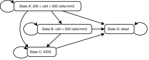
In this model the clinical condition of the patient is described by four possible states. State A, the least severe disease state, means that the CD4 count is between 200 and 500 cells/mm3. State B means less than 200 cells/mm3. State C represents AIDS and the final state, D,

represents death. The possible transitions are depicted as arrows in Figure 1. The cycle length is one year. The effectiveness is measured as life duration, without taking into account the quality of life.

Figure 1. Transition diagram for the HIV model.12

2.1

Qualitative information: structure of the model

A graph consists of nodes and links. MIDs, like decision trees and influence diagrams, have three types of nodes: decision, chance and value. If a node represents the value in the i-th cycle of a temporal variable, we write i between square brackets, as in Figure 2.

c

An Excel version of this model can be found on the web site for the book by Briggs et al.7:

www.herc.ox.ac.uk/downloads/supporting-material-for-decision-modelling-for-health-economic-evaluation/ex47sol.xls.

State A: 200 < cd4 < 500 cells/mm3

State C: AIDS

4

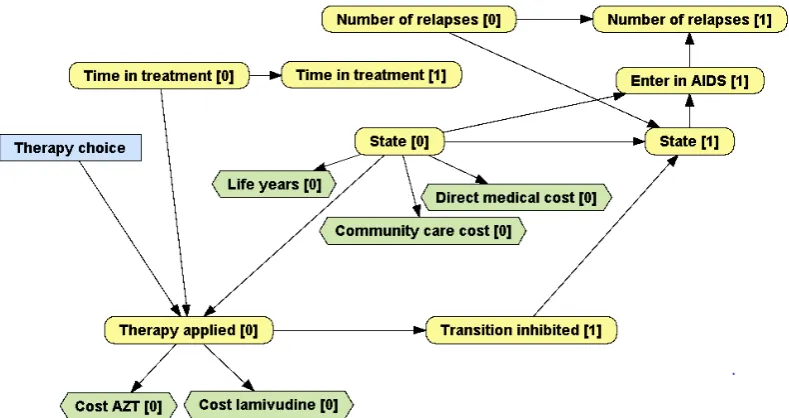
Figure 2. The first two cycles of an MID for the HIV example.

Decision nodes represent choices available to the decision maker. They are drawn as rectangles. In Figure 2, the decision node Therapy choice represents the selection of one of the two

therapies under evaluation. This node has no index because, as said above, we assume that all the decisions are atemporal.

Chance nodes, drawn as rounded rectangles, represent all the properties that are not under the decision maker’s control. In medical PGMs, they represent the patient’s features, such as sex, age and health condition at a certain moment.d Figure 2 contains 7 chance variables. State [0] represents the state of the patient in cycle 0 (start of therapy), with four values, one for each health state: A, B, C and D. State [1] represents the state of the patient in cycle 1 (one year later) and has the same domain as State [0]. Time in treatment [0] and Time in treatment [1] are numeric variables that represent, for each cycle, how much time the patient has been receiving treatment. Therapy applied [i] represents the therapy applied in the i-th cycle, which can be combination therapy, monotherapy or, if the patient is dead, none. Transition inhibited [1] indicates whether the addition of lamivudine has prevented a transition that would have occurred if the patient had received zidovudine (AZT) alone.

Value nodes represent the decision maker’s payoffs, such as costs and health outcomes. They are drawn as hexagons. In Figure 2, Life years [0] and Life years [1] represent effectiveness, while the other value nodes represent economic costs.

Nodes in an MID are connected by directed links. When there is a link , we say that is a parent of . These links usually denote causal influence. For example, Therapy applied [i] depends on Therapy choice, on State [i] (because dead patients do not receive any therapy) and on Time in treatment [i] (because combination therapy is applied for a maximum of two years and then all patients receive monotherapy). State [1] depends on State [0] and on whether the transition has been inhibited. The effectiveness (Life years [i]), the direct medical costs and the community care costs depend on the current state, while the cost of drugs depends on the therapy applied.

d_{This is a difference with decision trees, which do not represent patients’ baseline characteristics (for}

5

2.2

Quantitative information: numerical parameters

An MID, like any other PGM for decision analysis, contains two types of numeric parameters: probabilities and values. Each chance or value node has an associated potential, i.e., a function that assigns a real number to each configuration of a set of variables. The potential for a chance node is a probability distribution for that variable conditioned on its parents in the graph. The potential for a value node is a function that indicates how this value depends on its parents.

A potential defined on a set of n discrete variables can be encoded as an n-dimensional table. (In this context, discrete is synonymous of categorical or finite-states. A numeric variable can be discretised by defining a finite set of intervals.) In our example, the probability distribution for node State [0], which has no parents in the graph, depends on no variable, i.e., it is the a priori probability P(State [0]). In a cohort interpretation of the model, this probability represents the proportion of individuals in each state at the beginning of the treatment. As this variable has 4 states, the probability can be represented by a one-dimensional matrix (a vector) of 4 non-negative numbers, whose sum must be 1. The assumption that all the patients are initially in state A is encoded by setting the probability to 1 for this state and 0 for the others.

The probability of State [1] conditioned on its parents, State [0] and Transition inhibited [1], can be represented by a three-dimensional matrix, as shown in Figure 3.

Figure 3. Probability table for State [1], conditioned on State [0] and Transition inhibited [1]. The leftmost column lists the parents of State [1] and the four possible values of this variable. When the transition has been inhibited, the patient remains in the same state as in the previous cycle. A red triangle denotes second-order uncertainty; in this example there are three columns having each an associated Dirichlet distribution, which can be edited in a specific dialog.

6

Figure 4. A tree for P(Therapy applied [0] | State [0], Therapy choice, Time in treatment [0]). Even if the

therapy choice is “combination therapy”, the treatment reverts to monotherapy after the two first cycles.

The probability distribution for Time in treatment [0] is a Dirac delta because we know with certainty that the value of this variable is 0. Time in treatment [1] depends deterministically on its only parent, Time in treatment [0]; these two variables are related by a potential of type “cycle length shift”, so that the value of Time in treatment [1] is the value of Time in treatment [0] plus the cycle length.

The variable Transition inhibited [1] represents the effect of combination therapy, which in Chancellor’s model reduces the transition rate independently of the state of departure. Its probability is also represented by a table.

In the same way as every chance node has an associated conditional probability, every value node has a function that indicates how that value (the effectiveness or the cost) depends on its parents in the graph. In our example these functions can be represented by tables because they are all defined on discrete variables.

3

Building MIDs in practice

3.1

The process of building MIDs

An MID can be built by first drawing it on paper and then implementing it in a general programming language, such as C++, R or MATLAB. However, it is much easier to build it using a dedicated software package, such as OpenMarkov, because its graphical user interface facilitates the construction of the graph and the encoding of the potentials and because this tool offers efficient evaluation algorithms, as explained below.

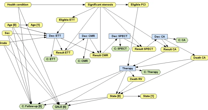
The first step in the construction of an MID is selecting the variables and assigning a domain to each decision and each chance variable. The next one is to draw links among the

nodes/variables, as explained in Section 2.1. Figure 5 and 6 show two MIDs containing two decisions (one about a test and one about a treatment) and several chance nodes that represent the patient’s personal characteristics, the health state, several symptoms, test results and

7

value nodes that represent effectiveness (quality of life) and economic costs. Please note that all the links represent either causality or functional dependence.

Figure 5. An MID for analysing the cost-effectiveness of the HPV vaccine, based on Callejo et al.13

8

The last step, the most difficult one, consists of assigning the potentials, especially those that contain numeric parameters. In Section 2.2 we have mentioned three types of potentials: table, tree and cycle length shift. There are two technical reports15,16 that describe in detail these and other types of relations and may serve as a guide for selecting the most appropriate

representation for each potential depending on the type of variables involved, on the data available and, sometimes, on the modeller’s preferences.

OpenMarkov’s tutorial (www.openmarkov.org/docs/tutorial) and ProbModelXML’s website (www.probmodelxml.org/networks) contain several examples that may be useful for both beginners and advanced modellers.

3.2

R

epresenting the patient s history

in MIDs

This section illustrates with two examples the use of memory variables in MIDs to represent the patient’s history without multiplying the number of states.

3.2.1 First example: Duration of stay in a certain state

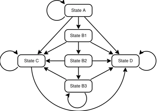
In some medical problems the transition probabilities depend on how long the patient has been in a certain state. For example, the longer an HIV patient has had a low CD4 count (state B), the higher the probability of developing AIDS (state C) or dying (state D). Therefore, Chancellor’s model can be refined by subdividing state B into three sub-states: B1, B2 and B3, such that B1 means that the patient has just entered state B, B2 that he entered state B in the previous cycle and B3 that he has been in state B for at least two cycles. States B1 to B3 are called tunnel states because they can be visited only in a fixed sequence,10 as shown in Figure 7.

Figure 7. A refined transition diagram for the HIV model (compare it with Figure 1). Sub-states B1, B2 and B3, called tunnel states because they can be visited only in a fixed sequence, indicate how long the patient has been in state B.

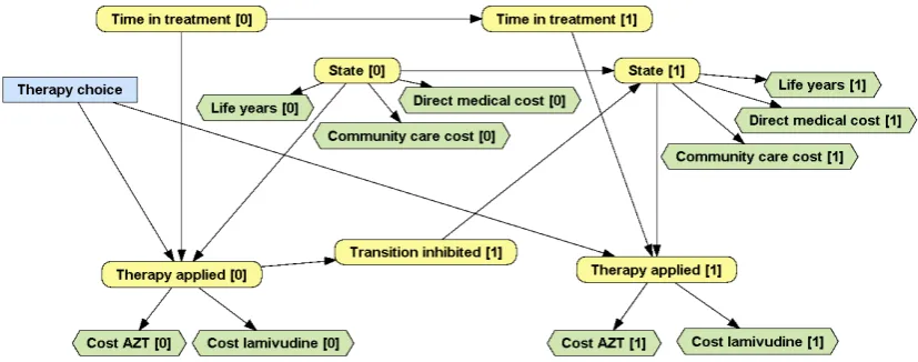
An alternative to using tunnel states is to represent the “state” with two variables: one for the clinical state—with four possible states: A, B, C and D, as in the original model—and another one for indicating how long the patient has been in the current state, as shown in Figure 8. The auxiliary variable State change [1] tracks whether there has been a transition in cycle 1. The link from Time in current state [0] to State [1] means that when the patient is in state B, the

State A

State B1

State B3

State B2 State D

9

transition probabilities to C and to D do not only depend on Therapy choice, but also on the time spent in B.

Figure 8. A refinement of the MID in Figure 2. The transition probabilities between State [0] and State [1] now depend on how many cycles the patient has spent in the current state. By definition, Time in current state [0] = 0. If State [1] takes the same value as State [0] , then State change [1] = false and Time in current state [1] = Time in current state [0] + 1; otherwise, State change [1] = true and Time in current state [1] is reset to 0.

The variables that summarise the history of the patient, such as Time in treatment [i] and Time in current state [i], are called memory variables. This way the transition probabilities may depend on the past without (explicitly) multiplying the number of states. Therefore, if State [i] has 4 values, Time in treatment [i] has m values and Time in current state [i] has n, this MID is equivalent to having 4· m·n states, but its construction and maintenance is much easier than building a traditional model with lots of states, because the user does not need to think of all the possible combinations of the variables that jointly represent the patient’s “state”.

3.2.2 Second example: Modelling relapses

In some cases the transition probabilities depend on the patient’s entire history. For example, a more up-to-date model for HIV should allow backward transitions from state C (AIDS) to A or B, due to the efficacy of modern treatments; the probabilities of these transitions depend on how many times the patient has had AIDS.

10

Figure 9. An alternative refinement of the HIV model that includes backward transitions. The subindex of a state indicates the number of relapses, i.e., the number of times the patient has entered state C; subindex 2 means that the patient has had AIDS at least twice.

An alternative approach would be to have one variable representing the clinical state and another one representing the number of relapses, as in Figure 10.

Figure 10. An MID accounting for the number of relapses in AIDS. When the patient transitions from states A or B into C, Enter in AIDS takes the value true and Number of relapses [1] = Number of relapses [0] + 1; otherwise Enter in AIDS = false and Number of relapses [1] = Number of relapses [0]. The transition probabilities from State [0] to State [1] depend on Time in treatment [0] and on Number of relapses [0] .

4

Algorithms for MIDs

An MID can be converted into an ordinary ID by expanding it to the desired horizon and then evaluated with the standard algorithms for IDs. For example, an MID containing only discrete variables—and numeric variables whose value is known with certainty, as in the HIV model— can be evaluated with the algorithm by Arias and Díez,6 which computes the incremental

cost-D

A0 A1 A2

C0 C1 C2

11

effectiveness ratios (ICERs) and the optimal strategy for each value of the willingness-to-pay.e If the MID has only one decision, this algorithm performs essentially the same operations as cohort evaluation, but it can also evaluate models containing several decisions, such as the examples in Figure 5 and 6. However, some MIDs having numerical variables may require patient-level simulation.

Similarly, it is possible to use variable elimination, a well-known algorithm for Bayesian networks and influence diagrams,17 to compute and display graphically the temporal evolution of a variable, as shown in see Figure 11. It is also possible to modify the parameters of the model and perform the same types of deterministic and probabilistic sensitivity analysis as with other types of models.

Given that the optimal policy for a decision depends on all the variables known when making it, the complexity of these algorithms grows exponentially with the horizon for MIDs containing temporal decisions, while it grows only linearly when all the decisions are atemporal. For this reason the MIDs presented in this paper and those available at

www.probmodelxml.org/networks only have atemporal decisions; all of them can be evaluated with OpenMarkov in less than 10 seconds.

Figure 11. Temporal evolution of different variables in the HIV model. a) Probability of each state of the variable State for combination therapy. b) Probability that the patient is alive, given by the sum of the probabilities of the states A, B and C of the variable State. c) Instantaneous value of Cost of drug, with 3.5% discount. d) Cumulative value of Life years, with 3.5% discount.

e

12

5

Comparison of MIDs with other representation techniques

5.1

MIDs vs. spreadsheet models

The most common tool for implementing state-transition models is Excel, at least in Europe,11 probably because this program is available in almost all computers, which avoids the need to buy dedicated software, and because it is relatively easy to write formulae in Excel. However, the more complex the model, the more Excel skills are needed, and sensitivity analysis is usually implemented by Visual Basic macros, which requires some knowledge of programming.

For a modeller, the main drawback is the need to encode the logic of the model in the form of sheets and formulae, which cannot be reused from other models. Additionally, in Excel models the state must be represented by a single variable because spreadsheets cannot deal with multidimensional matrices in a natural way. The only possibility of representing the patient’s history is to subdivide the states, as explained in Section 3.2 (Figure 7 and 9), and the more states in the model, the more difficult it is to build and maintain it. For this reason, when Hawkins et al.18 built a Markov model for the treatment of epilepsy, which needed to keep track of the time spent in the current state, they used R instead of Excel. In contrast, MIDs can represent the patient’s history with one or several memory variables, without multiplying the number of states.

The problem of Excel models is not only the effort required to write the formulae, but also the difficulty of uncovering the possible mistakes, because those formulae are more difficult to understand and debug than a piece of code written in a programming language. In fact, we detected minor bugs in four of the five Excel models that we translated into MIDs, even though their authors were in general experienced decision analysts. Fortunately, the impact of those bugs was irrelevant, but in other fields of scientific research there are notorious examples of Excel bugs that led to wrong conclusions.19-21In contrast, OpenMarkov’s code is periodically tested using modern software-engineering techniques and tools, and the probability that the modeller makes a mistake when building a model with a graphical user interface is much smaller than when writing formulae and macros that mingle the model with the inference algorithm.

For an evaluation agency, the main advantage of a model implemented as a spreadsheet is that the same file contains the model, the code and all the numerical results of its evaluation, thus making it possible to trace its execution step by step. However, the presence of complex

13

5.2

MIDs vs. Markov decision trees

Both decision trees and IDs, as well as their Markov extensions, are based on graphs containing three types of nodes: chance, decision and value; Markov decision trees have a fourth type of node, called Markov node. The main difference is that in (Markov) decision trees the links outgoing from a node represent the states of the corresponding variable, while links in IDs and MIDs represent causal relations. In general every variable appears several times in a decision tree, and the number of branches grows exponentially with the number of variables, which makes (Markov) decision trees inadequate for building large models. In contrast, in an MID each variable can appear at most twice (once for each of the first two cycles), and it is therefore much more compact than the equivalent Markov decision tree, in the same way as every ID is much more compact than the equivalent decision tree. The reader can appreciate the difference by trying to mentally build a Markov decision tree for the MIDs in Figure 5 and 6. For this reason, (M)IDs can solve much larger problems than (Markov) decision trees.

Additionally, when the dynamics of a model depends on the patient’s history, Markov decision trees have only two possibilities: to multiply the number of states, as in Figure 7 and 9, or to use so-called tracker variables. The first option leads to cumbersome models, just as when using Excel. The second requires patient-level simulation to evaluate the model, which often takes much longer than cohort analysis. In contrast, many MIDs containing memory variables, including all the examples shown in this paper, can be efficiently evaluated with the algorithm by Arias and Díez.6 Additionally, (M)IDs containing more than one decision are equivalent to (Markov) decision trees with embedded decision nodes, which cannot be evaluated with standard algorithms.3 These are other reasons for which Markov decision trees are inadequate for large problems.

With respect to software tools, the main package for building (Markov) decision trees and performing cost-effectiveness analysis is TreeAge Pro, a mature commercial product. Older programs, such as WinDM and SMLTREE, are no longer available. OpenMarkov, in contrast, is still a research prototype, but in addition to supporting MIDs and other types of probabilistic graphical models, has the key advantage of being open-source, which implies that it can be used for free, and also that its code can be inspected and extended to address the user’s needs.

Currently TreeAge Pro offers many features not available in OpenMarkov, but the latter has more and more features not available in the former.

5.3

MIDs vs. programming languages

Some state-transition models for cost-effectiveness analysis have been implemented in C++, MATLAB, R or a language in the BUGS family, such as WinBUGS, OpenBUGS or JAGS. The main advantage of this approach is the possibility of implementing virtually any model and any evaluation algorithm. The drawback is that, as in the case of Excel, the model is mingled with the algorithm and everything must be programmed by the decision analyst, from the

combination of transition probabilities to the sensitivity analysis and the graphical display of results.

14

From the point of view of an evaluation agency, assessing the validity of a model encoded as a computer program may be difficult, especially if the code lacks a good design, clear in-line comments and sufficient additional documentation.

Finally, we should mention that BUGS is especially suited for health technology assessment based on clinical trials because of its ability to integrate statistical inference and cost-effectiveness analysis, but building and evaluating a model is much harder than when using OpenMarkov. We have begun researching the integration of these tools, in order to combine the statistical power of the former with the facilities for model building and analysis of the latter; our goal is to use OpenMarkov to build the model, estimate its parameters from data (by connecting to some of the software packages in the BUGS family) and then perform cost-effectiveness and sensitivity analysis with the graphical user interface, without writing any code.

5.4

MIDs vs. discrete event simulations

Discrete event simulation (DES) is commonly used to model many entities that interact between them and with the environment;24 for example, several individuals that can transmit an

infectious disease to one another, or several beds in an emergency service to be occupied by patients who arrive randomly.

In the field of economic evaluation, some experts have argued that when a problem involves numeric variables or requires several variables to model the evolution of the patient DES is more appropriate than a state-transition model.24-29 However, we have shown that MIDs can easily address those problems without abandoning the paradigm of state-transition models. Additionally, many MIDs—including all those mentioned in this paper—can be evaluated with cohort analysis, which is in many cases more efficient than patient-level simulation.

The main limitation of MIDs is the assumption of discrete time, while in DES time can be either discrete or continuous, but it is unlikely that this difference may affect the conclusions of an economic evaluation.24

In summary, some problems that were previously supposed to require DES can be analysed with MIDs, thus maintaining all the advantages of state-transition models, which, according to a panel of experts, “may be simple to develop, debug, communicate, and analyze, and they readily accommodate the evaluation of parameter uncertainty”.30

6

Conclusions

Markov influence diagrams (MIDs) are a new type of probabilistic graphical model especially designed for cost-effectiveness analysis with state-transition models. They extend influence diagrams in the same way as Markov decision trees extend decision trees.

We have argued that most state-transition models implemented as spreadsheets or Markov decision trees can be built much more easily using MIDs. In particular, MIDs can use memory variables to summarise the patient’s history without multiplying the number of states.

15

of DES. Therefore MIDs can implement complex models that by far exceed the expressive power of spreadsheets without abandoning the paradigm of state-transition models, in which many health economists feel more comfortable.

For a decision analyst, building an MID and evaluating it with OpenMarkov is much easier and faster than implementing it as a spreadsheet, a Markov decision tree or a computer program, especially because its graphical user interface saves a lot of time and reduces the probability of making mistakes. Additionally, MIDs containing several decisions, such as the example in Figure 6, can be evaluated with the algorithm by Arias and Díez,8 which is difficult to implement in R or in another programming language, and virtually impossible in Excel or in patient-level simulation. However, there are other types of problems for which DES or dynamic transmission models are more adequate.

For an evaluation agency, understanding and assessing the correctness of an MID is much easier than for other types of models, for two reasons: because every MID is based on a causal graph that summarises the structure of the model, and because it can be inspected separately from the software code used to evaluate it.

Most of the advantages of MIDs depend on the availability of software with a graphical user interface for building and evaluating them. The only one currently available is OpenMarkov, an open-source package. Therefore in practice the applicability of MIDs is limited by the facilities offered by this tool, which is still a research prototype. It already offers a wide range of

potentials—including, for example, Weibull distributions and generalised linear models with fractional polynomials—and several types of deterministic and probabilistic sensitivity analysis; but if a problem required a feature not available in this tool, it would be impossible to build the model as an MID until that option is available. However, new features are constantly added to OpenMarkov, and other software packages might support MIDs in the future.

Acknowledgements

F.J.D., M.Y. and I.B. spent three months each at the Centre for Health Economics of the University of York, invited by Prof. Mark Sculpher. We thank him, Marta Soares and Claire Rothery for many comments and suggestions about this manuscript, and Susan Griffin, Paul Revill, Máirín Ryan, Quentin Summerfield and Simon Walker for sharing their models with us.

I.B. received a predoctoral grant from UNED. J.P. was financed by MED-EL GmbH and by a predoctoral FPU grant of the Ministry of Education, Science and Sport. The stays at the University of York were financed by a Santander Bank–UNED mobility grant (F.J.D.), the Ministry of Science and Technology (M.Y.) and UNED (I.B.). Our work was supported by the Spanish Ministry of Education and Science (grant TIN2006-11152), the Ministry of Science and Technology (TIN2009-09158), FONCICYT (no. 95185), the 7th Frame Programme (no. 262266 and FP7-PEOPLE-2012-IAPP-324401), the Health Institute Carlos III of the Spanish

16

References

1. Raiffa H. Decision Analysis. Introductory Lectures on Choices under Uncertainty. Reading, MA: Addison-Wesley; 1968.

2. Howard RA, Matheson JE. Influence diagrams. In: R. A. Howard, J. E. Matheson, eds. Readings on the Principles and Applications of Decision Analysis. Menlo Park, CA: Strategic Decisions Group; 1984:719-762.

3. Arias M, Díez FJ. The problem of embedded decision nodes in cost-effectiveness decision trees. Pharmacoeconomics 2014;32:1141-1145.

4. Kuntz KM, Weinstein MC. Modelling in Economic Evaluation. In: Drummond MF, McGuire A, eds. Economic Evaluation in Health Care. New York: Oxford University Press;

2001:141-171.

5. Arias M, Díez FJ. Cost-effectiveness analysis with sequential decisions. Technical report CISIAD-11-01. Madrid: UNED; 2011.

6. Arias M, Díez FJ. Cost-effectiveness analysis with influence diagrams. Methods of Information in Medicine 2015;54:353-358.

7. Briggs A, Claxton K, Sculpher M. Decision Modelling for Health Economic Evaluation. New York: Oxford University Press; 2006.

8. Gray AM, Clarke PM, Wolstenholme J, Wordsworth S. Applied Methods of Cost-Effectiveness Analysis in Healthcare. New York: Oxford University Press; 2011.

9. Siebert U, Alagoz O, Bayoumi A, et al. State-transition modeling: A report of the ISPOR-SMDM Modeling Good Research Practices Task Force-3. Medical Decision Making 2012;32:690-700.

10. Sonnenberg FA, Beck JR. Markov models in medical decision making: A practical guide. Medical Decision Making 1993;13:322-339.

11. Tosh J, Wailoo A. Review of software for decision modelling. Sheffield, UK: University of Sheffield; 2008.

12. Chancellor JV, Hill AM, Sabin CA, Simpson KN, Youle M. Modelling the cost effectiveness of lamivudine/zidovudine combination therapy in HIV infection. Pharmacoeconomics 1997;12:54-66.

13. Callejo D, Lopez-Polin A, Blasco J. Cost utility of human papilloma virus vaccine in Spain. Value in Health. 2010;13:A258-A258.

14. Walker S, Girardin F, McKenna C, et al. Cost-effectiveness of cardiovascular magnetic resonance in the diagnosis of coronary heart disease: An economic evaluation using data from the CE-MARC study. Heart 2013;99:873.

15. Díez FJ, Druzdzel MJ. Canonical probabilistic models for knowledge engineering. Technical report CISIAD-06-01. Madrid: UNED; 2006.

16. Arias M, Díez FJ, Palacios-Alonso MA, Bermejo I. ProbModelXML. A format for encoding probabilistic graphical models. Technical report CISIAD-11-02. Madrid: UNED; 2011.

17. Luque M, Díez FJ. Variable elimination for influence diagrams with super-value nodes. International Journal of Approximate Reasoning 2010;51:615-631.

17

19. Baggerly KA, Coombes KR. Deriving chemosensitivity from cell lines: Forensic bioinformatics and reproducible research in high-throughput biology. Annals of Applied Statistics 2009;3:1309-1334.

20. Herndon T, Ash M, Pollin R. Does high public debt consistently stifle economic growth? A critique of Reinhart and Rogoff. Cambridge Journal of Economics 2013;38:257-279.

21. Reinhart C, Rogoff K. Reinhart, Rogoff admit Excel mistake, rebut other critiques. Wall Street Journal Apr 17 2013.

22. Rennie D. Cost-effectiveness analyses: Making a pseudoscience legitimate. Journal of Health Politics, Policy and Law 2001;26:383-386.

23. Hill S, Mitchell A, Henry D. Problems with the interpretation of pharmacoeconomic analyses - A review of submissions to the Australian pharmaceutical benefits scheme. JAMA. 2000;283:2116-2121.

24. Karnon J. Alternative decision modelling techniques for the evaluation of health care technologies: Markov processes versus discrete event simulation. Health Economics 2003;12:837-848.

25. Davies R. An assessment of models of a health system. Journal of the Operational Research Society 1985;36:679-687.

26. Siebert U. When should decision-analytic modeling be used in the economic evaluation of health care? European Journal of Health Economics 2003;4:143-150.

27. Caro JJ. Pharmacoeconomic analyses using discrete event simulation. Pharmacoeconomics 2005;23:323-332.

28. Caro JJ, Getsios D, Möller J. Regarding probabilistic analysis and computationally expensive models: Necessary and required? Value in Health 2007;10:317-318.

29. Caro JJ, Briggs AH, Siebert U, Kuntz KM. Modeling good research Practices—Overview: A report of the ISPOR-SMDM Modeling Good Research Practices Task Force–1. Medical Decision Making. 2012;32(5):667-677.

30. Roberts M, Russell LB, Paltiel AD, et al. Conceptualizing a model: A report of the ISPOR-SMDM Modeling Good Research Practices Task Force–2. Medical Decision Making 2012;32:678-689.

31. Hazen GB. Dynamic influence diagrams: Applications to medical decision modeling. In: Brandeau ML, et al., eds. Operations Research and Health Care. Boston, MA: Kluwer Academic Publishers; 2004:613-638.