This is a repository copy of Evaluation of the integration of the Wind-Induced Flutter Energy Harvester (WIFEH) into the built environment: Experimental and numerical analysis.
White Rose Research Online URL for this paper: http://eprints.whiterose.ac.uk/121815/
Version: Accepted Version
Article:
Aquino, A.I., Calautit, J.K. and Hughes, B.R. (2017) Evaluation of the integration of the Wind-Induced Flutter Energy Harvester (WIFEH) into the built environment: Experimental and numerical analysis. Applied Energy. ISSN 0306-2619
https://doi.org/10.1016/j.apenergy.2017.06.041
Article available under the terms of the CC-BY-NC-ND licence (https://creativecommons.org/licenses/by-nc-nd/4.0/).
[email protected] https://eprints.whiterose.ac.uk/
Reuse
This article is distributed under the terms of the Creative Commons Attribution-NonCommercial-NoDerivs (CC BY-NC-ND) licence. This licence only allows you to download this work and share it with others as long as you credit the authors, but you can’t change the article in any way or use it commercially. More
information and the full terms of the licence here: https://creativecommons.org/licenses/
Takedown
If you consider content in White Rose Research Online to be in breach of UK law, please notify us by
The short version of the paper was presented at ICAE2016 on Oct 8-11, Beijing, China. This paper is a substantial extension of the short version of the conference paper.
1
Abstract 2
With the ubiquity of low-powered technologies and devices in the urban environment
3
operating in every area of human activity, the development and integration of a
low-4
energy harvester suitable for smart cities applications is indispensable. The multitude
5
of low-energy applications extend from wireless sensors, data loggers, transmitters
6
and other small-scale electronics. These devices function in the microWatt-milliWatt
7
power range and will play a significant role in the future of smart cities providing power
8
for extended operation with little or no battery dependence. This study thus aims to
9
investigate the potential built environment integration and energy harvesting
10
capabilities of the Wind-Induced Flutter Energy Harvester (WIFEH) – a microgenerator
11
aimed to provide energy for low-powered applications. Low-energy harvesters such as
12
the WIFEH are suitable for integration with wireless sensors and other small-scale
13
electronic devices; however, there is a lack in study on this type of technology’s
14
building integration capabilities. Hence, there is a need for investigating its potential
15
and optimal installation conditions.
16 17
This work presents the experimental investigation of the WIFEH inside a wind tunnel
18
and a case study using Computational Fluid Dynamics (CFD) modelling of a building
19
integrated with a WIFEH system. The experiments tested the WIFEH under various
20
wind tunnel airflow speeds ranging from 2.3 to 10 m/s to evaluate the induced
21
electromotive force generation capability of the device. The simulation used a
gable-22
roof type building model with a 27˚ pitch obtained from the literature. The atmospheric 23
boundary layer (ABL) flow was used for the simulation of the approach wind. The work
2
investigates the effect of various wind speeds and WIFEH locations on the
25
performance of the device giving insight on the potential for integration of the harvester
26
into the built environment. The WIFEH was able to generate an RMS voltage of 3 V,
27
peak-to-peak voltage of 8.72 V and short-circuit current of 1 mA when subjected to
28
airflow of 2.3 m/s. With an increase of wind velocity to 5 m/s and subsequent
29
membrane retensioning, the RMS and peak-to-peak voltages and short-circuit current
30
also increase to 4.88 V, 18.2 V, and 3.75 mA, respectively. For the CFD modelling
31
integrating the WIFEH into a building, the apex of the roof of the building yielded the
32
highest power output for the device due to flow speed-up maximisation in this region.
33
This location produced the largest power output under the 45˚ angle of approach, 34
generating an estimated 62.4 mW of power under accelerated wind in device position
35
of up to 6.2 m/s. For wind velocity (UH) of 10 m/s, wind in this position accelerated up
36
to approximately 14.4 m/s which is a 37.5% speed-up at the particular height. This
37
occurred for an oncoming wind 30˚ relative to the building facade. For UH equal to 4.7 38
m/s under 0° wind direction, airflows in facade edges were the fastest at 5.4 m /s
39
indicating a 15% speed-up along the edges of the building.
40
Keywords 41
Aero-elastic flutter; Buildings; Computational Fluid Dynamics (CFD); energy
42
harvesting; wind tunnel
43
1. Introduction 44
In this day and age, buildings are attributed for 20-40% of total world power
45
consumption. This is a figure greater than the consumptions of industry and transport
46
sectors [1]. Thus, new technologies that can mitigate the building sector power demand
47
are increasingly being advanced; one significant advancement being wind energy
48
technology. An important value of building-integrated wind energy harvesting is
49
bringing the power plant closer to the power consumers. With the public having better
50
power generation capabilities, people can also expect better energy efficiency and
51
reduced dependence to power companies, lower carbon footprint and general
52
stimulation of the economy. Moreover, this shift will decrease the load of the grid,
53
dependence on diesel generators in events of power outage and lower transmission
54
costs.
55 56
However, urban and suburban locations present problems for conventional
building-57
mounted turbines. There is the issue of significant turbulence in these areas, impeding
58
the turbines from harnessing laminar wind flow. In these conditions wind turbine
59
installers face insufficiency in analysing the more complex wind conditions. This leads
60
to problems of unfavourable turbine site selection leading to deficient power
61
production. Another issue that conventional rotational turbines face is the hazard of
62
having blades flying loose. These aspects add to the anxiety of turbine installation
63
among building owners, residents and stakeholders. However, perhaps the biggest
64
issue to building-integrated wind turbines (BIWT) is their cost-effectiveness. Smaller
65
wind turbines suitable for urban installations when installed onto buildings allow for a
66
higher cost-to-energy-production ratio.
67 68
A novel and emerging alternative to the conventional turbines are wind-induced flutter
69
energy harvesters. In this day and age, low-energy power generation devices have
70
been gathering increased attention because of their potential integration with
3
powered micro-devices and wireless sensor networks especially in the urban setting.
72
This is a primary motivation for this study. The power produced by these
73
microgenerators is sufficient to run light-emitting diodes, stand-alone wireless sensor
74
nodes and small liquid crystal displays [2]–[4]. Such devices like the Wind-Induced
75
Flutter Energy Harvester (WIFEH) as shown in Figure 1 can be in a form of a
small-76
scale wind generator that takes advantage of the flutter effect. Unlike turbine-based
77
generators, the WIFEH is a small-scale, light and inexpensive direct-conversion energy
78
harvester which does not use any gears, rotors or bearings. Wind flowing into and
79
around a tensioned membrane or belt causes it to flutter causing connected permanent
80
magnets to vibrate relative to a set of coils. This motion induces a current flowing in
81
the coil, thereby generating electric power.
82 83
Fig 1. Schematic diagram of a quad (4-coil arrangement) Wind-Induced Flutter
84
Energy Harvester (WIFEH)
85 86
The phenomenon of aero-elastic flutter describes self-feeding oscillations in which the
87
aerodynamic forces on a structure couple with its natural mode of oscillation thereby
88
producing rapid periodic movements. Flutter can occur to any structure exposed to
89
strong fluid flow, under the condition that a positive feedback response results between
90
the structure’s natural vibration and the acting aerodynamic forces [8].
91 92
Flutter on itself can be severely disastrous. Historic examples of flutter are the collapse
93
of Tacoma Narrows Bridge and that of Brighton Chain Pier. The structures failed due
94
to span failure caused by aero-elastic flutter [5]. However, this seemingly violent nature
95
of flutter can also be the foundation of its power when its potential for energy
96
harnessing is investigated. Flutter is classified under flow-induced vibrations, which is
97
an umbrella category that includes flutter-induced vibrations (FIV) [6]–[8] and
vortex-98
induced vibrations (VIV) [9]–[11].
99 100
Regular wind turbines generally don’t scale down well into smaller scales.
101
Nevertheless, flutter-based generators like the WIFEH can be designed to be suitable
102
for lighter applications. Low-energy flutter-based generators can operate in the range
103
of milliWatt to microWatt power generation. Although the power output is low, it has its
104
advantages compared to traditional wind turbines. The WIFEH is small, compact,
105
modular and suitable for turbulent flow, making it appropriate for partnering with
106
wireless sensor technologies – a field which has the greatest application potential for
107
this energy harvester [12]. Flutter energy harvesting is also not limited to
108
electromagnetic transduction, but can also be taken advantage of through the use
109
flexible piezoelectric membranes as demonstrated with an inverted flag harnessing
110
ambient wind to power a temperature sensor [13].
111 112
Recent world demand for wireless sensors is growing particularly in applications of
113
equipment supervision and monitoring focused on energy expenditure, usage, storage
114
and remote manipulation. The principal difficulties to what we call the “deploy
-and-115
forget” nature of wireless sensor networks (WSNs) are their restricted power capacity
116
and their batteries’ unreliable lifetimes. To surmount these problems, the area of
117
energy harvesting of ambient energy resources like air flow, water flow, vibrations, and
118
even radio waves has developed to be an encouraging new field. These and several
4
other types of ambient energy sources have been harnessed through various
120
technologies like thermomechanical, thermoelectric, photovoltaic and wind harvesting
121
technology [14]. There are even initiatives to develop micro-energy harvesters that can
122
harness both physical and chemical energies of the human body to power implanted
123
biomedical devices [15]. Along with developments in microelectronics, power
124
requirements for wireless sensor nodes keep on falling, varying presently from
125
microWatts to a few milliWatts [12].
126 127
In the year 2011, more than 1 million units of harvester modules were bought around
128
the world for building applications alone. This was mainly attributed to the expansive
129
network of wireless switches dedicated for lighting, air conditioning and sensors
130
detecting resident presence and determining ambient room conditions such as
131
humidity and temperature, mostly realised in commercial buildings. Running the
132
market growth of energy harvesters are the significant savings in installation costs and
133
maintenance-free operability due to little or no wire installation requirement [16].
134
Hence, novel methods should be established to further assess and optimise energy
135
harvester integration into the built environment. It has been shown that simple
136
configuration, low production cost and fast prototyping coupled with 3D-printing
137
technology all contribute to demonstrate practical applications of mini airflow-driven
138
energy harvesters in the urban setting [17].
139 140
In this paper, the evaluation of the energy harnessing potential of the WIFEH is
141
discussed. The evaluation is done two-fold: (i) through experimental investigation of
142
the harvester prototype conducted inside a wind tunnel; and (ii) through CFD analysis
143
relating external conditions and harvester location to harvester power generation
144
capabilities. The experimental analysis will assess a constructed WIFEH prototype’s
145
performance when subjected to different wind tunnel airflow velocities. The prototype
146
will be centrally mounted with the membrane allowed to flutter in the wind thereby
147
inducing relative motion between fastened permanent magnets and a fixed conducting
148
coil. This motion in turn induces an electromotive force (voltage) in the conducting coil.
149
The (root-mean-square) RMS and peak-to-peak voltages and current readings will be
150
recorded through a memory-enabled digital oscilloscope and afterwards analysed and
151
discussed.
152 153
Brief review of previous works on the WIFEH exposed that several authors have
154
assessed the performance of the device in uniform flows in the laboratory or wind
155
tunnel but did not investigate the effect of buildings on its performance. Therefore it is
156
evident that there exists the necessity of investigating the integration of the WIFEH into
157
buildings using CFD analysis.
158 159
The CFD analysis will investigate the effect of various external conditions and device
160
locations on the performance of the WIFEH. The simulation will use a gable-roof type
161
building model with a 27˚ pitch. The atmospheric boundary layer (ABL) flow will be 162
used for the simulation of the approach wind. The three-dimensional
Reynolds-163
averaged Navier-Stokes (RANS) equations along with the momentum and continuity
164
equations will be solved using ANSYS FLUENT 16 for obtaining the velocity and
165
pressure field. Sensitivity analyses for the grid resolutions of the CFD simulations will
166
be performed for verification of modelling. In addition, the results of the flow around the
5
buildings and surface pressure coefficients will be validated with previous experimental
168
work. Figure 2 shows the overview of how this study is organised.
169 170
Fig. 2. General organisation of the study
171
Section 1 introduces the overview of the project, the motivation, challenges, a brief
172
background of the technology and the direction of the research. Section 2 presents the
173
review of related literature. Section 3 discusses the experimental aspect of the study
174
evaluating the technology prototype inside a wind tunnel, while Section 4 presents the
175
results of CFD analysis of the device integration into buildings. Section 5 highlights the
176
key findings.
177
2. Literature Review 178
In this section, various relevant energy harvester technologies for flow-induced flutter
179
focusing on the electromagnetic generation principle are reviewed.
180 181
Pimentel et al. [18] investigated the operation of a wind flutter harvester via
182
experimental testing. The evaluated device was 50-cm long and supported by a
183
Plexiglass frame, with a tensioned Mylar membrane installed with bolts on its ends.
184
This membrane had one side that is smooth while the other side was rough. This is
185
analogous to a simple aerofoil. The generator had an electromagnetic transducer
186
integrated in one end of the membrane. This transducer utilised two small neodymium
187
(NdFeB) magnets and a static coil situated adjacent to the magnets. Based on the
188
investigators’ experimental results the minimum power output was 5 mW at wind speed
189
of 3.6 m/s and load resistance of 10 Ω; the maximum power output was 171 mW under
190
airflow of 20 m/s, 110 Ω resistance and 38.1 N membrane tension.
191 192
Several parameters that affect the wind flutter harvester performance like membrane
193
tension, membrane length, magnet position and number of magnets were investigated
194
by Arroyo et al. [19] using experimental methods. The study highlighted the optimal
195
values for the key parameters, focusing on low wind speeds ranging from 1 to 10 m/s
196
but with powerful vibration acceleration. Dinh Quy et al. [20] studied a wind flutter
197
harvester with the magnet positioned centrally along the flexible membrane made of a
198
type of kite fabric called ripstop nylon fabric. The single unit micro generator was able
199
to produce power in the range of 3 - 5 mW. Five larger versions of these
200
microgenerators were combined to produce a “windpanel”, which altogether were able
201
to deliver 30 to 100 mW of power at wind speeds less than 8 m/s. At low wind speeds
202
between 3 to 6 m/s, the output current is approximately 0.2 to 0.5 mA, the generated
203
voltage is between 2 to 2.5 V, and the generated power is about 2 to 3 mW, under
204
membrane oscillation frequency of approximately 5 Hz.
205 206
The earlier generations of flutter generators encountered practical problems as
207
identified by Fei et al. [21]. One example was the physical contact of the vibrating
208
membrane with the coils when its vibration amplitude is at an extreme high during
209
powerful winds. The placing of the magnets on the membrane should be thoroughly
6
tested to guarantee optimised magnetic flux undergone by the coils, which was also
211
addressed by Dinh Quy et al. [20].
212 213
To deal with these challenges and at the same time increase the efficiency of energy
214
harvesting by a fluttering belt, a novel variety of flutter-based resonant system was
215
proposed in [21] which involves of a shaft that acts as a support, an electromagnetic
216
resonator, a power management circuit, a super-capacitor for storage of charge and a
217
spring. A belt with dimensions 1 m long, 25 mm wide and 0.2 mm thick polymer was
218
used as the oscillating membrane. The electromagnetic resonator was positioned
219
close to the end of the membrane. This was the selected placement because of a
220
higher bending stiffness of the membrane close to the secured ends. This configuration
221
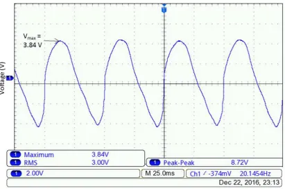
permitted a heavier magnet to be supported by the vibrating membrane [21]. The
222
super-capacitor is simply replaceable.
223 224
Dibin Zhu et al. [22] studied a device with an aerofoil linked to a beam which was
225
located next to a bluff body. This energy harvester worked under relatively low airflow
226
speed of 2.5 m/s and produced power of 470 W. The investigators found that a 227
drawback of this system was the factor that an initial displacement of the aerofoil was
228
required in order to be activated. Wang et al. [23] demonstrated a type of
EMG-229
resonant-cavity wind energy harvester integrated with dual-branch reed and tuning fork
230
vibrator. Their study emphasised the harvester’s magnetic circuit being able to 231
increase the rate of change of magnetic flux. The tuning-fork mechanism of the
232
harvester was able to reduce system losses. Apex power output was measured to be
233
56 mW corresponding to a wind speed of 20.3 m/s with efficiency of energy conversion
234
of 2.3% at wind speed of 4 m/s. The experimental tests verified that the harvester can
235
operate in a wide range of wind speeds.
236 237 238
Two types of electromagnetic energy harvesters were investigated by Kim et al. [24]
239
which utilise direct airflow energy conversion to mechanical vibration - (i) a
240
wind-belt-like oscillatory linear energy collector specially for powerful air streams and
241
(ii) a harvester involving a Helmholtz resonator concentrated on harvesting energy
242
from weaker airflow like those found in environmental air streams. The moving part of
243
the harvester was made up of an oscillating membrane with secured permanent
244
magnets, positioned in the centre of the airflow. The second energy collector utilised a
245
Helmholtz resonator as an apparatus for concentrating oncoming wind flow. The
wind-246
belt-like oscillatory energy collector offered a peak-to-peak amplitude AC voltage of 81
247
mV at frequency of 530 Hz, generating this from an input of 50 kPa of pressure. The
248
Helmholtz-resonator-centred harvester provided a peak-to-peak amplitude AC voltage
249
of 4 mV at frequency of 1400 Hz, from 0.2 kPa pressure input, which corresponded to
250
5 m/s or 10 mph airflow speed.
7
It was demonstrated by Munaz et al. [25]that the energy generation of electromagnetic
253
energy harvester can be amplified by several factors through the introduction of
254
numerous magnets as the moving mass despite the fact that all other experimental
255
parameters were fixed. The harvester generated power of 224.72 µW in rectified DC
256
already, while having a load resistance of 200 Ω for a five-magnet setup. This
257
electromagnetic energy harvester operated at a low resonance frequency of 6 Hz,
258
which was envisioned by the investigators to be suitable for handheld devices and
259
remote sensing applications.
260 261
Energy harvesting through vibrations caused by the Karman vortex street through an
262
electromagnetic harvester was investigated by Wang et al. [6], with a device able to
263
produce instantaneous power of 1.77 µW when exposed to the vortex street. The open
264
circuit peak-to-peak voltage induced in the coil was measured to be approximately 20
265
mV. In the same investigation the researchers acknowledged that the vibrations from
266
other fluid flow can also be harnessed such as river currents, air flow from tire or fluids
267
inside machinery.
268 269
Kwon et al. performed an investigation for energy harvesting devices that use
270
T-shaped cantilever intended to accelerate the occurrence of aero-elastic flutter for low
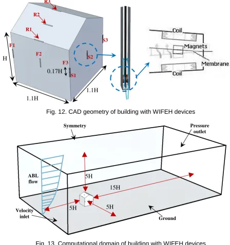
271
wind speeds. The investigators studied two device types – one working through
272
piezoelectric effect while the other operates under electromagnetic induction principle.
273
For the electromagnetic energy converter the cantilever is permitted to undergo flutter
274
thereby causing the motion of magnets with respect to coils, producing electricity in the
275
conducting coils. The devices were tested inside a wind tunnel and it was observed
276
that the electromagnetic converter was able to generate a maximum of 1.2 mW of
277
power under 10 m/s wind speed, while the piezoelectric device provided 1.5 mW
278
maximum power[26].
279 280
Park et al. investigated a technology with a funnel that was intended to contract wind
281
flowing towards the energy harvester. The study noted that aero-elastic flutter
282
phenomenon only starts when airflow speed reaches a specific flutter onset speed and
283
when airflow is nearly perpendicular to the harvester. The investigators’ solution was
284
to introduce a wind-flow-contracting funnel conceived to channel airflow to the flutter
285
energy converter and accelerate the airflow. The authors compared the device
286
performance under varying incident angles of wind and its effect on the voltage
287
generation for the device versions with funnel and without funnel. With the funnel, the
288
harvester produced almost a constant voltage even when the incident wind flow angle
289
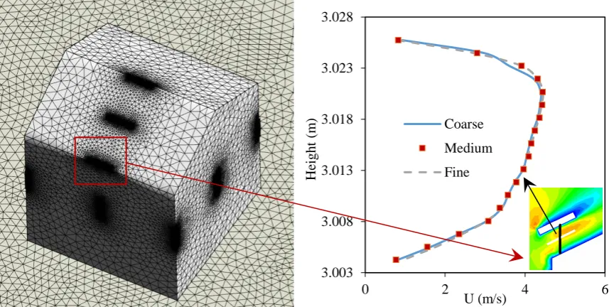
varied. The initial CFD and wind tunnel results also exhibited that the funnel can
290
accelerate airflow speed by an estimated 20% within an incident angle of 30º [27].
291 292
In another study by Arroyo et al. two significant parameters namely the critical flutter
293
frequency and the critical wind speed as functions of the ribbon dimensions and
294
material properties were focused on through utilising both theoretical modelling and
8
experiments. The important finding was that from both simulation and experiments, the
296
critical speed increased when the dimensions were reduced. Therefore a device
297
designed for low-speed airflow has to take into account this increase through
298
marginally decreasing the ribbon tension since the higher the ribbon tension is, the
299
greater the airflow speed required to start fluttering [28].
300 301
No previous work reviewed the integration of low-energy flutter-induced harvesting
302
devices in buildings or structures. Most studies for these energy harvesters were
303
carried out in laboratory environments. There is also a lack in numerical investigations
304
about these energy harvesting technologies. There is a deficiency in research about
305
the applications of these harvesters in the urban environment. Most theoretical studies
306
employ unrealistic boundary conditions like the use of uniform flows. This study will
307
address this by conducting an urban flow simulation of a small building integrated with
308
low-energy wind-induced flutter energy harvester devices and evaluate the impact of
309
varying outdoor wind conditions.
310 311
Prior investigations about the building environment’s potential for wind energy
312
harvesting underlined the necessity for detailed and precise analysis of wind flow
313
around buildings. To exploit the effect of wind acceleration above or around buildings
314
and to be able to determine the applicable type of wind energy technology to be
315
installed, appropriate integration analysis has to be conducted. In addition, there exists
316
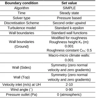
the challenge of analysing the optimum placement of the wind energy harvesters.
317
Thorough simulations will lead to more data that can result to better installation
318
decisions [29].
319
3. Performance evaluation of WIFEH prototype using wind tunnel testing 320
To characterise the effect of various wind speeds to the harvester’s performance, a 321
prototype was constructed and tested inside the wind tunnel. The prototype was tested
322
under varying wind tunnel airflow speeds to enable the measurement of RMS voltage,
323
peak-to-peak voltage and short-circuit current generated by the harvester in response
324
to the different wind velocities.
325 326
A full scale model of the WIFEH prototype was used in the experimental study. The
327
investigation was conducted in a low-speed closed-loop wind tunnel detailed in [30].
328
The wind tunnel had a test section with the dimensions of 0.5, 0.5, and 1 m (see
329
Figure 3). The variable intensity axial fan is capable of supplying wind speeds between
330
2.3 to 12 m/s. The flow in the wind tunnel was characterised prior to experimental
331
testing to indicate the non-uniformity and turbulence intensity in the test-section which
332
was 0.6% and 0.49% and according to the recommended guidelines [30].
333 334
Fig. 3. (a) Side view of the closed-loop wind tunnel (b) WIFEH prototype with one coil
335
configuration showing flutter motion at 2.3 m/s
336 337
The WIFEH system with one coil and eight stacked 1.5 mm-thick 10 mm-diameter
338
magnets was tested for preliminary experimental results inside the wind tunnel. The
339
prototype was positioned in a vertical orientation with terminals, as shown in Figure 4.
9
For data gathering, the system was connected to the digital oscilloscope positioned
341
outside the wind tunnel. It was ensured that the wind tunnel did not contain anything
342
except the WIFEH. The wind speed inside the tunnel was varied from the wind tunnel
343
minimum of 2.3 m/s to maxima of (i) 8 m/s without belt retensioning and (ii) 10 m/s with
344
belt retensioning. It should be noted that without retensioning, the performance of the
345
belt did not improve beyond 8 m/s. Without membrane retension there was observed
346
self-sustained but unstable oscillations leading to irregular voltage signal readings.
347 348
Fig. 4. Schematic of WIFEH prototype in the wind tunnel test section
349 350
The WIFEH was then connected to the Tektronix Oscilloscope to measure, display and
351
record the system’s AC (Alternating Current) voltage output. This is depicted in
352
Figure 5. The voltage waveform relevant characteristics such as the maximum value,
353
peak-to-peak voltage, root-mean-square (RMS) voltage and frequency could be
354
observed instantaneously in the 7-inch WVGA TFT colour display monitor. The
355
Tektronix TBS1052B Digital Storage Oscilloscope model is capable of up to 1 GS/s
356
sampling rate, bandwidths of 50 - 200 MHz and has a dual channel frequency counter.
357
The instrument has 3% vertical (voltage) measurement accuracy permitting the user
358
to see all signal details and obtain the stated real-time sampling rate on all channels
359
all the time with at least 10X over sampling; sampling performance is not reduced when
360
changing the horizontal (time) scale. The oscilloscope has two probes that were
361
attached to the two ends of the coils of the energy harvester, with one probe also
362
connected to the ground, to measure the potential difference between two points at
363
each specific time. Measurements were taken uninterruptedly producing a continuous
364
waveform that is displayed in oscilloscope’s LCD monitor and were recorded in a 365
storage device connected to the oscilloscope USB port.
366 367
Fig. 5. Schematic of the coil connections to the oscilloscope
368 369
The WIFEH model used for the wind tunnel testing was partially constructed using 3D
370
printing. The schematic diagram of the two-coil prototype system is shown in Figure 6.
371
The copper wire used to make the conducting coil is enamelled copper wire 40 SWG
372
(Standard Wire Gauge) with 0.125 mm diameter. It is packaged as grade 1 enamelled
373
copper wire in a roll of 250 grams and is suitable for coil forming. This copper wire is
374
tested based on the standards of IEC 851/5/4 having a threshold energy transfer rate
375
of 7 kVA (kilovolt-Amperes). The circular casing was 3D-printed using HP Designjet
376
3D Printer. The outer diameter of the casing is 54 mm and the inner diameter (hole
377
diameter) is 12.5 mm, with outer thickness of 20 mm and inner spacing for the coil
378
winding of 12 mm. The two ends of the coil wire were soldered onto insulated jumper
379
lead wires for more convenient connections to the load (LED) for initial testing of
380
generation, circuit board or testing apparatus. Approximately 2500 turns were looped
381
to produce the coil. The internal resistance of the coil is 1150 Ohms.
382 383
The flexible membrane is made of a two layer construction: a weather-resistant outer
384
shell and reinforced fabric backing. It resists moisture, UV rays and extreme
385
temperature. The backing material provides strength due to the tight weave. It adheres
386
to metallic objects well. It is highly suitable to hold the magnets in place, sturdy but light
387
and highly flexible allowing flutter to occur. In the tests it has not let the magnets fall
388
off in any trial done. A 1 cm wide section of the tape material of which 0.5 m in length
389
was exposed to airflow was used for the harvester. These dimensions were observed
10
to be suitable for the flutter occurrence to be initiated with the given load of the magnets
391
while keeping the use of the tape material economically, thereby reducing its weight.
392 393
Neodymium N52 type disk magnets were used to generate the magnetic fields that are
394
going to interact with the conducting coils. The magnets have a diameter of 10 mm and
395
a thickness of 1.5 mm. N52 is the highest grade for magnets that are widely available.
396
In a size for size comparison an N52 grade magnet will have approximately 35% more
397
pull power than the same sized N35 grade magnet. This type of magnet is axially
398
magnetised through the thickness producing one surface as the North pole and the
399
other surface being the south pole. Each unit weighs 0.09 g and has a coating of
Ni-400
Cu-Ni layers (Nickel-Copper-Nickel). The calculated maximum vertical hold of each
401
magnet is 206 g, having a theoretical maximum pull of 1033 g. The maximum operating
402
temperature of this type of magnet is 80°C, beyond which it will start to lose pa rt of its
403
magnetisation. Four units of the 1.5 mm thick magnets were stacked together which
404
are then attached to the adhesive side of the belt. It was estimated that four stacked
405
magnets will possess sufficient magnetic field strength strong enough to generate
406
substantial induction in the coils but at the same time not too heavy to hinder the belt
407
flutter motion. To balance the four magnets on one side, another four were attached
408
on the other side of the membrane with the opposite pole facing the first magnets stack
409
so that the magnetic attraction kept the two magnet groups in place.
410 411
Fig. 6. Schematic and dimensions of 3D-printed WIFEH prototype
412 413
The AC Voltage waveform produced by the WIFEH system when subjected to a
414
constant airflow of 2.3 m/s is shown in Figure 7, forming a regular pattern of sinusoidal
415
wave. This first trial corresponds to the initial and minimum flow velocity of the wind
416
tunnel. The root-mean-square (RMS) voltage was measured to be 3.00 V. The RMS
417
voltage is the effective value of a varying voltage source such as the WIFEH. The rated
418
output of most power supplies are expressed in RMS AC voltage (e.g. 110 / 230 V wall
419
socket output is RMS value). The maximum voltage reading was 3.84 V while the
peak-420
to-peak voltage was 8.72 V.
421 422
Fig. 7. Open-circuit voltage of the Wind-Induced Flutter Energy Harvester (WIFEH)
423
without membrane retensioning under 2.3 m/s flow velocity
424 425
Without prior retensioning the membrane, the wind tunnel airflow speed was increased
426
to 5 m/s and the AC voltage signal was again observed and recorded as shown in
427
Figure 8. The waveform is not as regular as for the previous case and we can observe
428
more occurrences of sharper turns with resemblance to sawtooth signals, with
429
decreasing magnitude of the negative peaks of the signal. The recorded RMS for 5
430
m/s wind speed is 4.16 V with peak-to-peak value 18.4 V and maximum value of 8.8 V.
431 432
Fig. 8. Electrical signal open-circuit voltage of the Wind-Induced Flutter Energy
433
harvester (WIFEH) without membrane retensioning under 5m/s flow velocity
434 435
The membrane of the WIFEH was then retensioned while maintaining the wind tunnel
436
airflow speed of 5 m/s. The AC Voltage waveform produced by the harvester system
437
when subjected to a constant airflow was again recorded. A regular pattern of
438
sinusoidal wave with minor and major peaks was again observed. Under this wind
11
condition, the microgenerator generated an RMS voltage of 4.88 V with maximum of
440
9.20 V and peak-to-peak value of 18.2 V. This is shown in Figure 9.
441 442
Fig. 9. Electrical signal open-circuit voltage of the Wind-Induced Flutter Energy
443
Harvester (WIFEH) with membrane retensioning under 5 m/s flow velocity
444 445
Incremental increases of 1 m/s airflow speed were also conducted for two cases: (i)
446
without belt retensioning (see Figure 10) and (ii) with belt retensioning (see Figure 11),
447
starting from 2.3 m/s. The open-circuit voltage and short-circuit current were then
448
observed using a digital multimeter after each incremental increase. The digital
449
multimeter used was the Proster VC99. It is an auto-ranging digital multimeter capable
450
of measuring AC/DC voltage and current, resistance, frequency and duty cycle, which
451
provides an LCD display.
452 453
It can be observed that for the case without belt retensioning the maximum open-circuit
454
voltage and short-circuit current both occurred for 6 m/s airflow speed, beyond which
455
there was a significant drop in both variables. This was due to the observation that
456
beyond said airflow speed the belt started to perform less stable oscillations compared
457
to cases of lower wind speeds. This unstable flutter greatly influences the
magnets-458
coil relative dynamic positioning, therefore affecting the induced voltage and current in
459
the conducting coil. Thus the relationship between airflow speed and open-circuit
460
voltage or short-circuit current was not observed to be linear (Figure 9). However, with
461
retensioning of the belt the linear relationship between airflow and voltage / current
462
resumed as can be seen in Figure 10. The trend continued even up to 10 m/s airflow
463
speed.
464 465
Fig. 10. Electrical output performance of the WIFEH without retensioning under
466
various flow velocities: (a) Open-circuit voltage (b) Short-circuit current
467 468 469
Fig. 11. Electrical output performance of the WIFEH with retensioning under various
470
flow velocities: (a) Open-circuit voltage (b) Short-circuit current
471 472
4. Computational Fluid Dynamics (CFD) analysis of WIFEH integration into 473
buildings 474
The basic assumptions for the numerical simulation include a three-dimensional, fully
475
turbulent, and incompressible flow. The flow was modelled by using the standard
476
k-epsilon turbulence model, which is a well-established method in research on wind
477
flows around buildings [31], [32]. The CFD code was used with the Finite Volume
478
Method (FVM) approach and the Semi-Implicit Method for Pressure-Linked Equations
479
(SIMPLE) velocity-pressure coupling algorithm with the second order upwind
480
discretisation. When the flow is not aligned with respect to the grid, more accurate
481
results are generally obtained by using the second order discretisation, especially
482
when dealing with complex flows. The general governing equations include the
483
continuity, momentum and energy balance for each individual phase. The standard
k-484
e transport model was used to define the turbulence kinetic energy and flow dissipation
485
rate within the model. The governing equations for the mass conservation (eqn. 1),
486
momentum conservation (eqn. 2), energy conservation (eqn. 3), turbulent kinetic
487
energy (TKE) (eqn. 4) and energy dissipation rate (eqn. 5) are summarised below:
12 489
(eqn.1)
where is density, t is time and u is fluid velocity vector.
490
(eqn.2)
where p is the pressure, g is vector of gravitational acceleration, is molecular dynamic
491
viscosity and is the divergence of the turbulence stresses which accounts for
492
auxiliary stresses due to velocity fluctuations.
493
(eqn.3)
where e is the specific internal energy, keff is the effective heat conductivity, T is the air
494
temperature, hi is the specific enthalpy of fluid and ji is the mass flux.
495
(eqn.4)
(eqn.5)
where is the source of TKE due to average velocity gradient, is the source of TKE
496
due to buoyancy force, and are turbulent Prandtls numbers, , and are
497
empirical model constants.
498
The geometry (Figure 12) was created using commercial CAD software and then
499
imported into ANSYS Geometry (pre-processor) to create a computational model. The
500
shape of the building was based on [32], which is a gable roof type building with a roof
501
pitch of 26.6°. The overall dimension of the building was 3.3 m (L) x 3 .3 m (W) x 3 m
502
(H). To create a computational domain, the fluid volume was extracted from the solid
503
model as shown in Figure 13. The fluid domain consisted of an inlet on one side of the
504
domain, and an outlet on the opposing boundary wall. The simulations were completed
505
using parallel processing on a workstation with two Intel Xeon 2.1 GHz processors and
506
16 GB fully-buffered DDR2 memory.
507 508
Fig. 12. CAD geometry of building with WIFEH devices
509
The computational domain size and location of model were based on the guideline of
510
COST 732 [33] for environmental wind flow studies. According to the guidelines, for a
511
single building with the height H, the horizontal distance between the sidewalls of the
512
building and side boundaries of the computational domain should be 5H. Similarly, the
513
vertical distance between the roof and the top of domain should also be 5H. In the flow
514
direction, the distance between the inlet and the façade of the building should be 5H
515
while for the leeward side and outlet, it should be 15H to allow the flow to re-develop
516
behind the wake region, as fully developed flow is normally assumed as the boundary
517
condition in steady RANS calculations [33] .
518 519
Fig. 13. Computational domain of building with WIFEH devices
520
.1
+
×
= 0
+ × = p + g + × ×
× ×
+ × = × ×
1 + × = × + +
.1 + × = × + 1 + 3 2
2
+ + +
13 521
4.1 Mesh design and verification 522
Due to the complexity of the model, a non-uniform mesh was applied to volume and
523
surfaces of the computational domain [34], [35]. The generated computational mesh
524
of the building model is shown in Figure 14. The grid was modified and refined
525
according to the critical areas of interests in the simulation such as the WIFEH. The
526
size of the mesh element was extended smoothly to resolve the areas with high
527
gradient mesh and to improve the accuracy of the results. The inflation parameters
528
were set according to the complexity of the geometry face elements, in order to
529
generate a finely resolved mesh normal to the wall and coarse parallel to it [36].
530 531
Fig. 14. (a) Computational grid (b) Sensitivity analysis
532 533
In this study, Grid Convergence Method (GCI) method was used to verify the
534
computational modelling of the building integrated with the WIFEH. The computational
535
grid was based on a sensitivity analysis which was performed by conducting additional
536
simulations with same domain and boundary conditions but with various gird sizes.
537
The process increased the number of elements between 2.44 (coarse), 3.8 million
538
(medium) and 4.90 million (fine). The computational time associated with running the
539
simulations (converged) with coarse, medium and fine mesh were 5 hours, 8 hours
540
and 10 hours, respectively.The grid resolution was determined taking into account an
541
acceptable value for the wall y+. The log-law, which is valid for equilibrium boundary
542
layers and fully developed flows, provides upper and lower limits of the acceptable
543
distance between the near-wall cell centroid and the wall. The distance is usually
544
measured in the dimensionless wall units, y+. The average y+ values over the
545
windward and the leeward roofs were about 70 and 25 for the coarser grid, and about
546
35 and 15 for the finer grid, respectively. The Grid Convergence Method (GCI) method
547
(based on the Richardson extrapolation method) was selected to estimate the
548
uncertainty due to discretisation [37]–[39]. The procedure detailed in [38] was followed
549
and is summarised below:
550
The first step is to define a representative grid size h.
551
(eqn.6)
where C is the total number of cells used for the 3D computations and is the
552
volume.
553
The next step is to select three significantly different set of grids, C and run simulations
554
to determine the values of key variables, . In this case, the average value of the
555
airflow velocity in the vertical line in the R1 device was selected as the variable. The
556
size of the grids were C1 (5.90 million), C2 (3.50 million) and C3 (2.00 million), giving
557
r values of 1.30 and 1.32.
558
= 1 (
=1
)
1/3
1 (
=1
)
14
The next step is to calculate the apparent order, p of the method using the next
559
equation. The equation was solved using fixed point iteration, with the initial guess
560
equal to the first term [38].
561
(eqn.7)
(eqn.8)
where = and = .
562
Finally, the approximate relative error , extrapolated relative error and fine-grid
563
convergence index (eqn.10) are calculated.
564
Table 1 shows examples of the calculation procedure for the three selected grids.
565
According to Table 1, the numerical uncertainty in the fine-grid solution for the velocity
566
at 3.012m was 2.68% which corresponded to ± 0.10 m/s.
567
Table 1. Sample calculations of discretisation error using the GCI method
568
Figure 15 (a) shows the vertical velocity profiles (line with 18 equally distributed points)
569
drawn from the R1 device, which was based on the three set grids. In addition, the
570
extrapolated values, are also plotted and was calculated using the following
571
equation:
572
(eqn.9)
The local order of accuracy p ranged from 0.95 to 16.1. The average apparent order
573
of accuracy was used to assess the GCI index values in eqn.11, which is plotted in
574
the form of error bars, as shown in Figure 4b. Based on the fine-grid convergence
575
index, the maximum discretisation uncertainty was 5.87%. The discretisation
576
uncertainty value ranged from 0.31% to 6.61%, with a global average of 1.52%.
577
(eqn.10)
Fig. 15. Grid verification using the Grid Convergence (GCI) method. (a) plot of the
578
velocity profiles drawn from a line in the R1 device; (b) fine grid solution, with
579
discretisation error bars computed using the GCI index.
580
4.2 Boundary conditions 581
The boundary conditions were specified according to the AIJ guidelines [40]. The
582
profiles of the airflow velocity U and turbulent kinetic energy (TKE) were imposed at
583
the inlet which were based on [32], with the stream-wise velocity of the approaching
584
flow obeying the power law with an exponent of 0.25 which corresponds to a sub-urban
585
terrain (See Figure 16). The values of for the k-epsilon turbulence model were
586
acquired by assuming local equilibrium of Pk = [32]. The standard wall functions [41]
587
were applied to the wall boundaries except for the ground, which had its wall functions
588
adjusted for roughness [42]. According to [42], this should be specified by an equivalent
589
= 1
ln( 21) 32 21
+ ( )
( ) = 21 1 × 32 21
32 1 × 32 21
) 32 213 2 21 2 1
21 21
21
21
21 =1.25 21
15
sand-grain roughness height ks and a roughness constant Cs. The horizontal non
590
homogeneity of the ABL was limited by adapting sand-grain roughness height and
591
roughness constant to the inlet profiles, following the equation of [43] :
592
(eqn.11)
593
where z is the aerodynamic roughness length of the sub-urban terrain. The values
594
selected for sand-grain roughness height and a roughness constant 1.0 mm and 1.0
595
[32]. The sides and the top of the domain were set as symmetry, indicating zero normal
596
velocity and zero gradients for all the variables at the side ant top wall. For the outlet
597
boundary, zero static pressure was used. The boundary conditions for the CFD model
598
are summarised in Table 2.
599 600 601
Fig. 16. (a) Velocity profile (b) TKE profile of approach wind flow [32] 602
603 604
Table 2. Summary of the CFD model boundary conditions
605 606 607
The convergence of the solution and relevant variables were monitored and the
608
solution was completed when there were no changes between iterations. In addition,
609
the property conservation was also checked if achieved. This was carried out by
610
performing a mass flux balance for the converged solution. This option was available
611
in the FLUENT flux report panel which allows computation of mass flow rate for
612
boundary zones. For the current simulation, the mass flow rate balance was below the
613
required value or <1% of smallest flux through domain boundary (inlet and outlet).
614
4.3 Method verification and validation 615
Figure 17 shows a comparison of the result of different turbulence model (k-epsilon
616
standard, k-epsilon realizable and k-omega) for the velocity profile drawn from the
617
vertical line in the R1 device. It can be observed that the k-epsilon standard curve lies
618
between the plots of k-epsilon realizable and k-omega, which is especially noticeable
619
between the heights of 3.005 and 3.015 m. It is obvious that there is an occurring
620
speed-up within the interior zone of the WIFEH device regardless of the turbulence
621
model used, as can be observed from Figure 17 (b). Although shifting to the k-omega
622
model could potentially affect the performance results of the WIFEHs located in the
623
leeward side of the building; a higher set of velocity results could be generated leading
624
to greater output for the devices in case of k-omega model.
625
As observed in Figure 17 (a), a very similar trend can be noticed for different turbulence
626
models particularly the k-epsilon standard and realizable with an average error of 3.9%
627
between the points. The average error between k-epsilon standard and k-omega was
628
6.44. From the velocity contours shown in Figure 17 (b) it can be noticed that the
629
k-epsilon standard model also displays mode distinguishable and more evenly
630
distributed velocities at a lower speed at the wake of the flow behind the structure,
631
compared to the k-omega model. The k-epsilon model provides the standard, mostly
632
accepted results and is more suitable when studying free-shear layers and wake zones
633
while the standard k-omega model is more suitable in the near wall boundary regions.
16 636
637
Fig. 17. Sensitivity analysis of turbulence model (a) velocity profile in R1 (b) velocity
638
contours
639 640
Figure 18 (a) and (b) show a comparison between the experimental PIV results of [32]
641
and the current modelling results of the velocity distribution around the building model.
642
The results of the airflow velocity close to the windward wall seem to be at a lower
643
speed in the model compared to the PIV results, however a similar pattern was
644
observed for most areas particularly close to the roof. Figure 18 (c) and (d) show a
645
comparison between the prediction of the current model and [32] of the pressure
646
coefficient distribution around the building model. It is to be noted that the contour of
647
Figure 18 (a) also apply to that of (b), while that of Figure 18 (c) apply to (d).
648 649
Fig. 18. (a) PIV measurements of velocity [32] (b) velocity distribution in the current
650
model (c) pressure coefficient result [32] (d) pressure coefficient distribution in the
651
current model
652
4.4 CFD results and discussion 653
The system of the aero-elastic belt energy harvester integrated into a building was
654
modelled using CFD through ANSYS Fluent simulating the airflow pattern, velocity
655
magnitude and distribution around the building and within and surrounding the energy
656
harvester. This was conducted to allow for optimisation of the positioning of the energy
657
harvester throughout the various building sections. This investigation simulated a
658
gentle breeze, which is category 3 in the Beaufort wind force scale.
659 660
Figure 19 shows the velocity contours of a side view cross-sectional plane inside the
661
computational domain representing the airflow distribution around the building
662
integrated with WIFEH. The left hand side of the plot shows the scale of airflow velocity
663
in m/s. The contour plot in the fluid domain is colour coded and related to the CFD
664
colour map, ranging from 0 to 5.9 m/s. As observed, the approach wind profile entered
665
from the right side of the domain and the airflow slowed down as it approached the
666
building and lifted up. Separation zones were observed on the lower windward side of
667
the building and also at the leeward side of the building and roof. Zoomed in views of
668
the velocity distribution around the WIFEH devices R1, R2 and R3 are shown on top
669
of the diagram. The results showed that the shape and angle of the roof had a
670
significant impact on the performance of the WIFEH. In the diagram, it is clear that
671
locating the device at the leeward side of the roof will result in little to no energy
672
generation due to the low wind speeds in this area. However, it should be noted that
673
this was not the case for other wind angles, for example when the wind is from the
674
opposite direction. Therefore, location surveying, wind assessment and detailed
675
modelling are very important when installing devices in buildings. At wind velocity (UH)
676
4.7 m/s and 0° wind direction, the airflow speed in R1 was the highes t at 4.5 m/s while
677
the lowest was observed for the R2 WIFEH located at the centre of the roof.
678 679
Fig. 19. Contours of velocity magnitude showing a cross-sectional side view of the
680
building
17
Figure 20 displays the velocity contours of a top view cross-sectional plane inside the
683
computational domain representing the airflow distribution around the building
684
integrated with WIFEH. The approach wind profile entered from the right side of the
685
domain and the airflow slowed down as it approached the building and accelerated as
686
it flowed around the corners. Separation zones were observed on the leeward side of
687
the building and also the sides. Zoomed in views of the velocity distribution around the
688
WIFEH devices F1-F3 and S1-S3 are shown on top and right side of the diagram. At
689
wind velocity (UH) 4.7 m/s and 0° wind direction, the airflow speed in F1 and F3 were
690
the highest at 5.4 m/s while the lowest was observed for the S2 and F2 WIFEH located
691
at the airflow recirculation zones.
692
Fig. 20. Contours of velocity magnitude showing a cross-sectional top view of the
693
building
694
Figure 21 compares the maximum air velocity speed measured at the belt location for
695
roof installations R1, R2 and R3 at various wind directions. These setups behaved in
696
a trend similar to each other, but the notable highest velocities were attained from the
697
R3 or apex installation. These setups had peak velocity values occurring at the region
698
between 30˚ to 60˚ orientation, with the maximum value obtained at 30˚. There was 699
significant speed decrease after 60˚ that could be attributed to the belt frame corners
700
which impeded the wind from flowing through the belt region and therefore would
701
reduce its performance or not allow the belt to flutter
702
Fig. 21. Effect of wind direction on the wind speed at WIFEH located on the roof for
703
various wind angle of approach with outdoor wind UH = 10 m/s
704
705
Figures 22 and 23 compare the maximum air velocity speed measured at the device
706
location for the windward and side installations, respectively at various wind directions.
707
When comparing the two figures it was observed that the plot of F3 had a similar trend
708
with the S1 device which showed a significant performance drop in terms of velocity
709
between 20-60˚. This was also due to the frame of the WIFEH which impeded the wind
710
from flowing through the belt region and therefore would reduce its performance or not
711
allow the belt to flutter.
712 713
While the plot of F1 was a mirrored of S3, and F2 was mirrored S2. There is some
714
symmetry that can be expected as observing the locations in Figure 12. It is not a
715
perfect symmetry due to the roof shape having some effect on airflow. Looking at the
716
location with highest velocity values for the front side of the building, there was a
717
significant decrease in velocity from 10˚ to 40˚, accounting for approximately 83% 718
speed reduction, and same increase in speed was observed from 40˚ to 70˚. For the 719
side installation S1 the tipping point was at 50˚ where the change in angle exposure
720
past this point marked significant increase in velocity. From the results it was clear that
721
both the location of the device and wind direction had a significant effect on the air
722
speed achieved at the device location. Therefore a complete detailed analysis of these
723
factors should be carried out when integrating WIFEHs to buildings to ensure that the
724
performance is optimised.
18
Fig. 22. Effect of wind direction on the wind speed at WIFEH located on the windward
726
side of building with outdoor wind at UH = 10 m/s
727
Fig. 23. Effect of wind direction on the wind speed at WIFEH located on the side of
728
building with outdoor wind at UH = 10 m/s
729
730
Figure 24 illustrates the effect of different outdoor wind speed UH values of 2, 4, 6, 8,
731
and 10 m/s at 0° wind direction on the air speed achieved at the de vice location. Similar
732
trend was observed for all the curves with the highest speed achieved in R1 and F3
733
and lowest speed achieved in F2 and S2. The increase in the velocity profile
734
corresponded to a proportional increased for the wind speed for all the device
735
locations.
736 737
Fig. 24. Wind speeds gathered at WIFEH position for various mounting locations for
738
0° wind angle of approach
739 740
Figure 25 depicts velocity results for 90° wind angle approach. At this angle the output
741
of the roof installations were overtaken by those in the front and side, most notably by
742
F3, S1 and S3 mainly because of the geometry of the device frame. The frame restricts
743
airflow in the perpendicular direction to the device. Therefore for locations with this
744
type of prevailing wind direction it will be better for the WIFEH to be integrated through
745
the front and side edges of the building.
746 747
Fig. 25. Wind speeds gathered at WIFEH position for various mounting locations for
748
90° wind angle of approach
749 750
Figure 26 compares the estimated output of the device at various locations and wind
751
directions of 0 to 90˚, in increments of 10 degrees while maintaining a uniform outdoor 752
wind velocity (UH = 10 m/s). F1, F2 and F3 represent the WIFEH devices mounted on
753
the front face of the building; S1, S2 and S3 represent those on the side face, while
754
R1, R2 and R3 are those for the roof locations. As observed, the highest power output
755
comes from location R3 – the apex of the building – with an estimated output of 15.2
756
V, resulting from wind speed that accelerated up to approximately 14.4 m/s,
757
approximately 37.5% speed-up at the particular height. This occurred for an incoming
758
wind 30˚ relative to the building facade. 759
760
Depending on prevailing wind direction of the area, the installation location of the
761
device can be determined. The green trendline represents the power output trend for
762
R3, the location with the highest total power generation summed over 0 to 90 degrees.
763
The brown trendline shows the trend for S2, the location with the lowest summed power
764
generation over the same angular range.
765 766
Secondary to the building apex, locations on the edge also provide well above-average
767
power output. Based on the simulated conditions, locations S3, F1 and R1 should be
768
optimum locations for building integration of the WIFEH, considering the power
769
averages for 0, 45 and 90-degree orientations.
770 771
The last locations an installer would want to put an WIFEH on are the central areas of
772
the building’s faces (illustrated by F2 and S2). Taking into account angular averages
19
these locations provided the least amount of power, with no power generated at all for
774
some cases due to the wind speed not being able to make it to the WIFEH’s cut-in
775
wind speed for generation. This finding can be considered by some to be a
776
counterintuitive result, considering these locations are directly hit by the oncoming
777
wind.
778
Fig. 26. Sample calculation of estimated voltage output based on WIFEH
(2-magnet-779
coil system)
780
781
Figure 27 compares the estimated output of the device located in the three locations
782
F3, S3 and R3 at various outdoor wind speeds. Among these three locations, at 30°
783
wind direction, R3 provided the highest output ranging between 2.5 to 15.2 V, while F3
784
showed the lowest output.
785 786
Fig. 27. Impact of various outdoor wind speeds (UH) on the estimated output of the
787
WIFEH for locations F3, S3 and R3
788
789
From the results it was clear that both the location of the device and wind direction had
790
significant effects on the air speed achieved at the belt locations. Therefore a complete
791
and detailed analysis of these factors should be carried out when integrating
aero-792
elastic belts to buildings to ensure that the performance is optimised. Certain changes
793
in angle exposure past certain critical values marked significant increase in velocity
794
and consequently, power generation.
795
5. Conclusions and future works 796
The Wind-Induced Flutter Energy Harvester is valuable for low-energy wind harvesting
797
in the built environment due to its low cost and modularity. The following points
798
encapsulate the important findings of the study:
799
With increasing airflow speed came increases in open-circuit voltage and
short-800
circuit current produced by the WIFEH. Regular sinusoidal waveform voltage
801
signals were observed through a digital oscilloscope for wind tunnel airflow
802
speeds of 2.3 m/s and 5 m/s with the belt retensioned.
803
The RMS (effective) voltages recorded were 3.0 V and 4.88 V with maximum
804
values of 3.84 V and 9.20 V for 2.3 m/s and 5 m/s wind tunnel airflow speeds,
805
respectively.
806
The simulation used a gable-roof type building model with a 27˚ pitch obtained
807
from the literature. The atmospheric boundary layer (ABL) flow was used for the
808
simulation of the approach wind. At wind velocity (UH) 4.7 m/s and 0° wind
809
direction, the airflow speed in R1 was the highest for the roof section at 4.5 m/s.
810
At wind velocity (UH) 4.7 m/s and 0° wind direction, the airflow speed in F1 and
811
F3 were the highest for the façade and side sections at 5.4 m/s.
812
The overall highest power output comes from location R3 – the apex of the
813
building – with an estimated output of 15.2 V, resulting from wind speed that
814
accelerated up to approximately 14.4 m/s, approximately 37.5% speed-up at
815
the particular height. This occurred for an incoming wind 30˚ relative to the 816
building facade.


![Fig. 16. (a) Velocity profile (b) TKE profile of approach wind flow [29]](https://thumb-us.123doks.com/thumbv2/123dok_us/7727310.161981/36.595.99.499.52.320/fig-velocity-profile-tke-profile-approach-wind-flow.webp)
