This is a repository copy of
Consumer surplus for random regret minimisation models
.
White Rose Research Online URL for this paper:
http://eprints.whiterose.ac.uk/125762/
Version: Accepted Version
Article:
Dekker, T orcid.org/0000-0003-2313-8419 and Chorus, CG (2018) Consumer surplus for
random regret minimisation models. Journal of Environmental Economics and Policy, 7 (3).
pp. 269-286. ISSN 2160-6544
https://doi.org/10.1080/21606544.2018.1424039
(c) 2018 Journal of Environmental Economics and Policy Ltd. This is an Accepted
Manuscript of an article published by Taylor & Francis in Journal of Environmental
Economics and Policy on 17 Jan 2018, available online:
https://doi.org/10.1080/21606544.2018.1424039
[email protected] https://eprints.whiterose.ac.uk/ Reuse
Items deposited in White Rose Research Online are protected by copyright, with all rights reserved unless indicated otherwise. They may be downloaded and/or printed for private study, or other acts as permitted by national copyright laws. The publisher or other rights holders may allow further reproduction and re-use of the full text version. This is indicated by the licence information on the White Rose Research Online record for the item.
Takedown
If you consider content in White Rose Research Online to be in breach of UK law, please notify us by
1
Consumer surplus for random regret minimisation models
1
Thijs Dekker* 2
Institute for Transport Studies, University of Leeds 3
36-40 University Road, Leeds, LS2 9JT, United Kingdom 4
[email protected] ; 0044-1133435330 5
Caspar G. Chorus 6
Transport and Logistics Group, Delft University of Technology 7
Jaffalaan 5, 2628BX, Delft, the Netherlands 8
[email protected], 0031-152788546 9
* Corresponding author 10
Abstract
11
This paper is the first to develop a measure of consumer surplus for the Random Regret Minimisation 12
(RRM) model. Following a not so well-known approach proposed two decades ago, we measure 13
(changes in) consumer surplus by studying (changes in) observed behaviour, i.e. the choice probability, 14
in response to price (changes). We interpret the choice probability as a well-behaved approximation of 15
the probabilistic demand curve and accordingly measure the consumer surplus as the area underneath 16
this demand curve. The developed welfare measure enables researchers to assign a measure of consumer 17
surplus to specific alternatives in the context of a given choice set. Moreover, we are able to value 18
changes in the non-price attributes of a specific alternative. We illustrate how differences in consumer 19
surplus between random regret and random utility models follow directly from the differences in their 20
behavioural premises. 21
22
Key words: Random Regret Minimisation; Consumer Surplus; welfare; probabilistic demand function; 23
2
1. Introduction
1
McFadden (1981), Small and Rosen (1981), and Hanemann (1984) were amongst the first to establish 2
the theoretical connection between discrete choice modelling, specifically the Random Utility 3
Maximisation (RUM) model, and welfare economics. Batley and Ibanez (2013a) provide a 4
comprehensive overview of this literature, but more importantly also provide five assumptions under 5
which the indirect utility function is consistent with economic theory. Additive Income RUM (AIRUM; 6
McFadden 1981), for which the indirect utility function is linear in prices and income, adheres to these 7
five assumptions and provides discrete choice modellers with its most well-known monetary measure 8
of consumer surplus, i.e. the LogSum (e.g. Cochrane, 1975; De Jong et al. 2007). 9
10
In discrete choice models, (changes in) choice probabilities are an appropriate way to reflect (changes 11
in) behaviour in response to price or quality (changes). When demand is restricted to unity and the Batley 12
and Ibanez (2013a) assumptions are fulfilled, then the choice probability can be interpreted as a 13
probabilistic demand curve. Williams (1977) and Ben-Akiva and Lerman (1985) accordingly calculate 14
(changes in) the area underneath the demand curve to derive a Marshallian measure of consumer surplus 15
which coincides with the Hicksian LogSum measure under AIRUM (e.g. McConnell 1995). 16
17
The five assumptions put forward by Batley and Ibanez (2013a) are, however, conflicting with many of 18
the behavioural phenomena observed in recent empirical studies, such as compromise effects (e.g. Boeri 19
et al. 2012), cost damping (e.g. Batley 2016), heterogeneity in cost sensitivities across goods (e.g. Hess 20
et al. 2007) and non-linear income effects (e.g. Dagsvik and Karlström 2005) to name a few. By relaxing 21
some of the aforementioned assumptions we may be able to better explain empirically observed 22
behaviour. However, the resulting functional form for the choice probabilities can no longer be 23
interpreted as probabilistic demand functions since they no longer provide a solution to what is known 24
in the economic literature as the ‘integrability problem’ (e.g. Deaton and Muellbauer 1980). As a result,
25
welfare analysis based on such inconsistent indirect utility functions is limited; or sometimes argued to 26
3 Relaxing some of the aforementioned assumptions requires giving up the notion of a fully rational 1
consumer. This is a direct result of incorporating elements of irrationality, such as compromise effects 2
as done by the Random Regret Minimisation (RRM) model (Chorus 2010), in the deterministic part of 3
the ‘indirect utility’ function used to estimate discrete choice models. This is in line with the notion that
4
not all irrational behaviour would be captured by the existence of an error term in the RUM model. A 5
potential solution emerges when one follows a line of reasoning proposed by McConnell (1995), who 6
states that “If there is a change in behaviour, there is also most likely a change in welfare”. In other 7
words, if one is willing to accept that a model is viable representation of (potentially irrational) choice 8
behaviour, this opens a door towards meaningful welfare analysis, albeit – as we will show below – in 9
a limited number of cases. 10
11
The perspective we adopt is simple. Although for the behavioural phenomena described above choice 12
probabilities are still well-defined and they behave consistently and in a predictable fashion with respect 13
to price and quality changes, these choice probabilities can no longer be interpreted as probabilistic 14
demand functions. However, if we treat them ‘as if they were’, we are able to develop a monetary
15
analogue to the traditional Marshallian consumer surplus. Such an approximation will be inherently 16
imperfect and reflects the price paid for adopting a behavioural economics approach. We will discuss 17
its limitations in more detail in Section 5. The developed measure allows evaluating, in monetary terms, 18
the existence value of environmental goods and welfare implications of changes in these environmental 19
goods. 20
21
In this paper, we particularly focus on the Random Regret Minimisation (RRM) model (Chorus 2010). 22
It is well-known for its ability to take compromise effects in individual decision-making into account 23
(e.g. Guevara and Fukushi 2016). The compromise effect arises in the RRM since bad performance on 24
one environmental attribute (e.g. water quality) can hardly be compensated by a very good performance 25
on another attribute (e.g. easy access).1 The incorporation of RRM in the NLOGIT and Latent GOLD
26
1 Some readers may be familiar with Regret Theory (Loomes and Sugden 1982). The RRM model is distinctively
4 software packages (EconometricSoftware 2012; Vermunt and Magidson 2014), and its inclusion in the 1
second edition of the Applied Choice Analysis textbook (Hensher et al. 2015), can be considered 2
evidence of the growing interest in RRM among scholars and practitioners, including those in the field 3
of environmental economics (e.g., Thiene et al., 2012; Boeri et al., 2012; Adamowicz et al., 2014). This 4
provides a context for exploring to what extent meaningful welfare measures can be derived for RRM 5
models, something which is especially important in the field of environmental economics. Our approach 6
extends to more recently proposed generalizations of RRM (e.g., van Cranenburgh et al., 2015), as well 7
as to other choice models incorporating attributes of competing alternatives in an alternative’s value 8
function (e.g., Chorus and Bierlaire 2013; Leong and Hensher 2015; Guevara and Fukushi 2016). 9
10
Section 2 defines the challenges arising when measuring consumer surplus for the RRM and other non-11
utility theoretic models. Section 3 sets out to meet these challenges and Section 4 illustrates our approach 12
with an empirical application. Not surprisingly, the behavioural properties of the RRM model have a 13
direct impact on the derived welfare measures. Differences between RUM and RRM welfare measures 14
can be substantial, and can be easily be traced back to the shape of the regret function. Section 5 15
discusses the interpretation and limitations of the obtained welfare measures. The proposed measure is 16
most relevant when applied to choice situations with a well-defined set of choice alternatives, such as 17
mode or route choice alternatives. Section 6 concludes and provides directions for future research. 18
19
2. A brief introduction into consumer surplus and random regret
20
2.1 Welfare effects for utility functions linear in price
21
For ease of exposition, we start by adopting an AIRUM indirect utility function Ui for alternative i in
22
(1) which is linear in price pi and income Y. Its deterministic component Vi also comprises a function
23
5 of non-price attributes Xi characterising the alternative. is the vector of parameters relating Xi to
1
Vi through . Furthermore, i captures the unobserved elements of the utility function independent of
2
price, income and quality. The latter is typically defined as a random variable. We assume i to be
3
identically and independently distributed and to take the form of a Type I Extreme Value Distribution 4
such that choice probabilities can be described in the form of the multinomial logit model (e.g. Train 5
2009). 6
7
(1)
8
9
In this indirect utility function, it can be observed that represents both the marginal disutility of price 10
and the marginal utility of income. It can be easily verified that the above specification satisfies all five 11
assumptions described in Batley and Ibanez (2013a). As such, the behaviour described by (1) is 12
consistent with a consumer maximising his direct utility subject to a monetary budget constraint Y. Using 13
the properties of duality, i.e. the possibility of rewriting the utility maximisation problem as a 14
expenditure minimisation problem, the Slutsky equation allows separating demand responses to price 15
(or quality changes) in so-called income and substitution effects. This separation is important in 16
understanding the difference between Hicksian and Marshallian consumer surplus measures. 17
Marshallian consumer surplus embodies both income and substitution effects as it is related to observed 18
changes in demand. Because of including income effects, the Marshallian welfare measure can be 19
subject to the issue of path dependency (e.g. Batley and Ibanez 2013b). The Hicksian compensating 20
variation filters out the income effect by looking into how much income can be taken away from (or has 21
to be given to) a consumer after a price or quality change has taken place to make him indifferent 22
between the original and new situation. Following Herriges and Kling (1999) we can define the 23
compensating variation CV in (2) where J refers to the choice set and the superscripts ‘0’ and ‘1’ 24
respectively define the utility before and after the change.2 Due to the unobserved nature of , the
25
2 The Hicksian equivalent variation (EV) takes the new utility level as the point of departure and examines how
6 compensating variation is a random variable for which typically the expected value is derived for the 1
purpose of social welfare analysis. 2
3
max max (2)
4
5
It turns out that for the adopted AIRUM indirect utility function the CV in (3) is defined by the difference 6
in the expected maximum utility before and after the improvement divided by , i.e. the marginal utility 7
of income (e.g. Small and Rosen 1981). For the multinomial logit model the expected maximum utility 8
is defined by the ‘LogSum’ (e.g. Cochrane, 1975; De Jong et al. 2007). Note that the unknown constant
9
C in (3) drops out when identifying changes in expected maximum utility. 10
11
(3) 12
13
Williams (1977) provides an interesting perspective on obtaining the Marshallian consumer surplus, 14
also discussed by Ben-Akiva and Lerman (1985). Here, the choice probability i for alternative i is
15
viewed as the observed probabilistic demand function for alternative i. A change in environmental policy 16
will have an impact on the vector of indirect utilities V. Accordingly, the change in consumer surplus 17
arising from a change in environmental policy improving alternative i can be defined by (4). As 18
described by Ben-Akiva and Lerman (1985), the integral is defined in utility terms and a common money 19
metric, in our case , is required to translate this utility surplus into monetary terms.3
20
21
(4) 22
23
The implemented linear relationship between income (price) and utility ensures that the Marshallian 24
consumer surplus following any order of price changes is path independent, i.e. does not exhibit income 25
7 effects (Batley and Ibanez 2013b).4 As a result, the Marshallian consumer surplus, the Hicksian
1
compensating variation and the equivalent variation measures are identical. Welfare calculations are 2
possible for choice models with more flexible error specifications. For example, the family of 3
Multivariate Extreme Value models have closed form solutions that are reformulations of the LogSum 4
formula. Finally, ‘translational variance’ allows ignoring Y in (1) during estimation without influencing 5
choice probabilities and welfare estimates.5 The inclusion of Y here is illustrative as it makes explicit
6
that consumers derive additional utility from spending their residual income on the numeraire good. 7
8
2.2 The restrictiveness of the economic framework
9
Section 2.1 illustrates that a well-defined economic framework governs the use of the LogSum as a 10
measure of consumer welfare. The underlying assumptions significantly restrict the scope for 11
introducing flexible indirect utility functions in estimation. Violations of the Batley and Ibanez (2013a) 12
assumptions may arise quicker than one may expect. If such violations occur, the labelling of U as an 13
indirect utility function, is incorrect as the connection with a rational consumer maximising his or her 14
direct utility subject to a budget constraint no longer holds. This poses choice modellers with a trade-15
off between behavioural relevance and the possibility of conducting meaningful welfare analysis. 16
Behavioural relevance allows researchers to exploit the wide range of econometrically possible 17
formulations of the ‘indirect utility function’, i.e. the regression equation defining the attractiveness of
18
a specific alternative. Batley and Dekker (2017), mathematically and graphically show that in the context 19
of a discrete choice models, where demand is restricted to unity, non-linear income effects are not 20
consistent with economic theory. Any additional income must be spent on the numeraire good which by 21
definition has to be path independent, i.e. not subject to an income effect. 22
23
4 Technically, if the absolute value of prices affect the choice probabilities, then this is an indication of an income
effect (Jara-Diaz and Videla 1989).
5Adding to every alternative in the choice set does not affect choice probabilities since choice probabilities
8
2.3 The RRM model - attribute level differences and non-linearity
1
We set out to develop an approximation of the Marshallian consumer surplus for the Random Regret 2
Minimisation (RRM) model as presented in equation (5). A detailed description of the RRM model is 3
provided in Chorus (2010), and a review of the model’s core properties and empirical comparisons
4
between RRM and RUM models can be found in Chorus et al. (2014). 5
6
ln exp ln exp (5)
7
8
The RRM model in (5) is particularly interested in differences in attribute levels across alternatives. 9
That is, regret R (alternatively interpretable as the negative of (decision) utility) arises when alternative 10
i is outperformed by alternative j on attribute m. The consumer is assumed to select the alternative with 11
the lowest level of regret and is a parameter to be estimated for attribute m. The RRM treats attribute 12
level differences in a non-linear fashion such that the marginal regret of being outperformed by another 13
alternative on attribute m is increasing in the level of the attribute level difference. The behavioural 14
justification for this non-linearity can be found in extremeness aversion (Simonson and Tversky 1992) 15
where people are argued to dislike extremely ‘bad’ attribute level performance and in loss aversion in
16
riskless choice contexts (Tversky and Kahneman 1991) where losses with respect to a reference point 17
(in this case: another alternative’s attribute level) weigh heavier than gains. As a result of this model
18
specification, the RRM model is able to account for choice set composition effects and tends to predict 19
higher market shares for so-called compromise alternatives with an intermediate performance on every 20
attribute (e.g. Chorus and Bierlaire 2013, Guevara and Fukushi 2016).6 The RRM model clearly
21
represents a decision model based in behavioural decision theory (Edwards 1961; Slovic et al. 1977; 22
Einhorn and Hogarth 1981) rather than economics. 23
24
6 The non-linear specification of the RRM model enables estimation of a dispersion parameter in the logit
9 Unlike the AIRUM model, the RRM model does not exhibit a connection between income and utility. 1
It is not a valid indirect utility function as it offers no opportunity to reflect a reduction in regret 2
achieved by spending residual income on the numeraire good. In effect, it lacks a common money 3
metric to transform changes in regret into monetary welfare measures. Formally, if we assume 4
then for any income level the binary regret function reduces to 5
ln exp ln exp . Regret arising from
6
differences in disposable income between any pair of alternatives remains solely determined by the 7
underlying price differences between these two alternatives. A lump-sum increase in income will 8
therefore have no impact on regret. 9
10
Note that the specification of the regret function in terms of non-linear attribute level differences is 11
significantly different from the non-linear in price utility functions considered in e.g. Dagsvik and 12
Karlström (2005); Herriges and Kling (1999); Karlström and Morey (2001); McFadden (1995). The 13
referred papers have explored methods to derive the (Hicksian) compensating variation in the presence 14
of income effects. Typically, simulation methods are required, but Dagsvik and Karlström (2005) and 15
de Palma and Kalani (2011) provide analytical formulae. These Hicksian measures, however, appear 16
not to be utility theoretic per the work of Batley and Dekker (2017) and Batley and Ibanez (2013a, 17
2013b). 18
19
A distinguishing feature of the RRM model which poses challenges for the derivation of consumer 20
surplus, is that a deterioration in attribute xim increases the regret of alternative i, but simultaneously
21
decreases the regret of all other alternatives j ≠ i. Hence, not only the current users of (or those who 22
switch to) alternative i are affected by the change in xim.
23
24
In the next section, we use the regret function in (5) to develop three specific cases of the RRM-based 25
analogue of the Marshallian consumer surplus. First, it defines the welfare effects of changing the price 26
10
set. Third, based on McConnell’s method we are able to value changes in non-price attributes. The
1
approach allows researchers to extract additional welfare information from RRM models that have 2
already been estimated. 3
4
3.
Consumer surplus in the RRM model
5
3.1 Changing the price of a single alternative
6
As mentioned in the introduction section, we acknowledge that RRM-based choice probabilities are not 7
consistent with the economic definition of a Marshallian (i.e. observed) probabilistic demand function. 8
We only interpret it as such since choice probabilities provide the best information available on changes 9
in behaviour in response to price and quality changes. We initially focus on the welfare effect of a change 10
in the price of alternative i. By focusing on a price change, our approximation of the Marshallian 11
consumer surplus is directly expressed in monetary terms. Where Ben-Akiva and Lerman (1985) take 12
the integral over changes in indirect utility resulting from the price change, we take the integral with 13
respect to the change in prices. Please note the resemblance with standard micro-economics (Neuberger 14
1971; Harris and Tanner 1974) which also measures the Marshallian consumer surplus as the area 15
underneath the uncompensated demand curve with respect to price. In line with the law of demand 16
choice probabilities i(pi) are expected to fall in prices. Equation (6) describes the change in consumer
17
surplus as a result of the change in pi.
18
19
(6)
20
21
Choice probabilities are well-defined in the RRM model and typically take the multinomial logit form 22
(e.g. Chorus 2010; Chorus et al. 2014), but do not comply with the Independence of Irrelevant 23
Alternatives axiom even when random errors are i.i.d. Appendix A confirms that RRM-based choice 24
probabilities are monotonically decreasing in pi such that the probabilistic demand function for
25
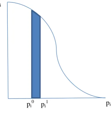
11 Figure 1 illustrates the reduction in monetary consumer surplus arising from an increase in pi. Note that
1
in the RRM model the change in choice probability is not only caused by an increase in the regret of 2
alternative i, but also by a simultaneous reduction in regret of all other alternatives j ≠ i. Changes in pi
3
might have a minor impact on Ri, but the change in Rj may be large such that i is still affected. By
4
focusing on changes in probability rather than compensating for changes in regret our approach 5
significantly differs from the indifference based approach to marginal welfare measurement in the RRM 6
model discussed by Dekker (2014). 7
pi
i
pi0 pi1
[image:12.595.120.309.260.451.2]8
Figure 1: Reduction in consumer surplus as a result of a price increase in pi
9 10
3.2 Value of having an alternative in the choice set
11
McConnell (1995) points out that the preceding logic can also be used to determine the value of having 12
(access to) a particular alternative in the choice set (up to a constant). Namely, by increasing the price 13
of an alternative (by means of introducing a hypothetical tax ti or alternative price levy) the associated
14
choice probability i reduces to zero. The consumer surplus Ci of having alternative i in the choice set
15
(within either a RUM or RRM model) is then defined by the integral over all possible positive values of 16
ti , i.e. the price increase, and denotes the amount of money that can be collected from the individual
17
before demand reduces to zero. 18
19
(7)
12 McConnell (1995) showed that for the AIRUM model the integral in (7) has a closed form solution equal 1
to , where again represents the marginal utility of income and
i0 the probability of2
selecting alternative i in the original situation 0. In practice, this is an alternative mathematical 3
formulation of the LogSum. Integrating down to zero demand as McConnell (1995) suggests, assumes 4
that the estimated model is valid at extremely low choice probabilities. The corresponding price levels, 5
however, may lie outside the normal range over which models are estimated. The inclusion of a choke 6
price (e.g. Morkbak et al. 2010) might address this problem in order to avoid making assumptions about 7
model behaviour in unobserved areas. The latter is an empirical rather than a theoretical matter and is 8
not restricted to the RRM model. 9
10
The differences between the linear-in-all-attributes RUM and the RRM model manifest themselves 11
when J > 2.7 First, they provide a different starting point, i.e. choice probability, to (7). Second, the
12
shape of the probabilistic demand function varies between the two models. The marginal change in the 13
RUM-based choice probability due to levying a tax is given by (8). This change in iRUM is largest when 14
0.5
RUM i
due to entropy. For the RRM model, the corresponding derivative is given by (9). For large 15
ti, the derivative approaches lim
1
1
i
RRM
RRM RRM i
i i M
t i J t
from below since limi 0
j t i R t and
16 lim i i M t i R t
. The size difference between and (J-1) M then determines whether the choice
17
probability in the linear-in-attributes RUM or RRM has a fatter tail. Faster convergence to a zero choice 18
probability reduces the consumer surplus of an alternative. 19
20
1
0 for 0RUM RUM RUM i i i i t
(8)
21
1
0RRM
j
RRM RRM RRM
i i
i j i
j i
i i i
R R
t t t
(9)22
13
3.3 Valuing changes in the attributes of a single alternative
1
Now moving to our third type of consumer surplus: changes in consumer surplus (i.e., the change in 2
existence value of the alternative) as a result of changing the attribute levels of alternative i. When 3
introducing changes in the non-price attributes of alternative i, the probabilistic demand curve in Figure 4
1 shifts rather than that a change along the probabilistic demand curve is made. Accordingly, the change 5
in consumer surplus cannot be simply obtained by integrating over the change in price. McConnell 6
(1995) shows that the probabilistic demand function can, however, still be applied to derive this 7
particular change in value. Equation (10) then measures the difference in existence value between the 8
new and original situation as denoted by the superscripts ‘1’and ‘0’ respectively. This formulation can
9
be applied to RUM, RRM and other well-behaved specifications of the choice model. 10
11
1 0
0 0
i i i i i i i
CS t dt t dt
(10)12
13
McConnell shows that for the AIRUM model, the change in consumer surplus is then given by 14
1
0
1 0 ln 1 i ln 1 i i i i
CS C C
, where the 0 and 1 refer to respectively the value before and 15
after the change in attribute levels of alternative i. Not surprisingly, this is a simple reformulation of the 16
difference in the LogSum between the two situations. 17
4.
Empirical illustration
18
To illustrate our concepts of consumer surplus in the RRM model, we use a dataset on route choice as 19
discussed in Chorus and Bierlaire (2013). Section 4.1 discusses the dataset and estimates a linear-in-20
parameters and attributes RUM and an RRM model. Section 4.2 derives the value of having access to a 21
particular route. Section 4.3 derives the welfare implications of improving or deteriorating the travel 22
time on a particular route. The welfare calculations for the RUM model have a closed form solution as 23
discussed in Section 3. For the RRM model this is also the case, but we prefer to numerically 24
14 too much scope for programming error. MATLAB’s built in integral() function is used for the purpose 1
of numerical approximation. 2
4.1 The Chorus and Bierlaire (2013) route choice dataset
3
The Chorus and Bierlaire (2013) datasets comprises 390 respondents, all members of a Dutch internet 4
panel maintained by IntoMart. All respondents owned a car, were employed and over 18 years old. The 5
sampling strategy was designed to ensure that the sample was representative for the Dutch commuter in 6
terms of gender, age and education level. The response rate was approximately 71 % and the data were 7
collected in April 2011. 8
9
Each respondent was presented with nine choice tasks in which they were requested to choose between 10
three different routes for their commute that differed in terms of the following four attributes, with three 11
levels each: average door-to-door travel time (45, 60, 75 min), percentage of travel time spent in traffic 12
jams (10, 25, 40 %), travel time variability (5,15, ± 25 min), and total costs (5.5, 9, €12.5).
13
The choice tasks were then generated using a ‘optimal orthogonal in the differences’ design (Street et
14
al. 2005). 15
16
Table 1 provides an overview of the estimated model parameters for a linear-in-parameters RUM model 17
and the RRM model. All parameters are of the expected sign and it can be observed that > 2 M such
18
that for very expensive alternatives the choice probability in the RRM model is decreasing more rapidly 19
than in the RUM model, in the context of this dataset. In Sections 4.2 and 4.3 we will focus on two 20
specific choice tasks (see Table 2), one with and one without a clear compromise alternative. We expect 21
that in the case of the former differences between the welfare effects between the RUM and RRM model 22
are larger due RRM’s possibility to capture compromise effects.
23
15
Table 1: Estimation results for a basic RUM and RRM MNL model
1
Linear RUM model RRM model
Parameter estimate t-value Parameter estimate t-value
Average travel time -0.0673 -35.02 -0.0468 -33.31
Percentage of travel time in congestion -0.0273 -17.17 -0.0181 -16.68
Travel time variability -0.0316 -12.04 -0.0210 -12.00
Travel costs -0.173 -20.64 -0.1128 -19.79
Observations 3,510 3,510
Loglikelihood -2,613 -2,605
[image:16.595.60.526.80.212.2]2
Table 2: Examples of choice-tasks featuring a compromise alternative and one without
3
Task: Alternative B acts as a compromise alternative Route A Route B Route C
Average travel time (minutes) 45 60 75
Percentage of travel time in congestion (%) 10% 25% 40%
Travel time variability (minutes) ±5 ±15 ±25
Travel costs (€) €12.5 €9 €5.5
YOUR CHOICE
Task: no clear compromise alternative Route A Route B Route C
Average travel time (minutes) 60 75 45
Percentage of travel time in congestion (%) 10% 25% 40%
Travel time variability (minutes) ±15 ±25 ±5
Travel costs (€) €5.5 €12.5 €9
YOUR CHOICE
4
4.2 Existence value of particular route
5
The model parameters and attribute levels are combined to derive the model specific choice probabilities 6
(see Table 3), which serve as starting points for (7). The compromise alternative, Route B in the first 7
choice set, as expected receives a market share bonus in the RRM model compared to the RUM model. 8
Consequently, the other alternatives comprising more extreme attribute levels are assigned a lower 9
choice probability in the RRM model. Choice probabilities are more comparable between RUM and 10
RRM in the second choice set, in the absence of a clear compromise alternative. These differences in 11
starting points are also reflected in the alternative specific CS measures presented in Table 3. In the first 12
choice set, Routes A and C are valued higher in the RUM model than in the RRM model as a result of 13
their higher choice probabilities. Since alternative A is the most expensive alternative in the choice set, 14
its RRM-based CS is particularly low due to the high level of marginal regret caused by price increases 15
[image:16.595.68.523.230.428.2]16 due to being a compromise alternative. The additional popularity of Route B results in a €0.14 increase 1
in consumer surplus (existence value). Despite being cheap, alternative C is not very popular in both the 2
RUM and RRM model and is therefore assigned a rather low consumer surplus in both models. 3
[image:17.595.60.525.197.371.2]4
Table 3: Value of the alternatives in the two choice sets presented in Table 1 (in euros)
5
Choice set 1 Observed RUM RRM
Choice share
i E(CS) Std. 2.5% 97,5% i E(CS) Std. 2.5% 97,5%
Route A 68% 70% 7.00 0.49 6.09 8.03 67% 5.51 0.43 4.72 6.42 Route B 27% 23% 1.49 0.08 1.35 1.65 27% 1.63 0.07 1.49 1.78
Route C 5% 7% 0.44 0.04 0.37 0.52 6% 0.38 0.03 0.32 0.45
Choice set 2 RUM RRM
Choice share
i E(CS) Std. 2.5% 97,5% i E(CS) Std. 2.5% 97,5%
Route A 54% 51% 4.14 0.22 3.73 4.59 53% 4.49 0.22 4.08 4.94
Route B 2% 3% 0.16 0.02 0.12 0.20 2% 0.12 0.02 0.09 0.16 Route C 44% 46% 3.61 0.27 3.12 4.16 45% 3.36 0.24 2.92 3.88 * Standard deviations and confidence intervals obtained using the Krinsky and Robb (1986,1990) method with 10,000 draws from the original variance covariance matrix of parameter estimates.
6
Also for the second choice set the consumer surplus measures differ across alternatives and behavioural 7
models. For example, having access to Route A is valued €4.14 by the RUM model and €4.49 by the 8
RRM model. The higher value of Route A in the RRM model can be explained by its higher choice 9
probability and good performance in terms of price (implying a low marginal regret for marginal price 10
increases caused by the tax levy). Again, this results in lower choice probabilities, and hence access 11
values, for the other two routes relative to the RUM model. 12
13
4.3 Changes in the travel time on a route
14
We illustrate the use of (10) by respectively improving and deteriorating (see Tables 4 and 5) the average 15
travel time of the routes presented in Table 2 by five minutes.8 The non-linearity of (10) with respect to
16
average travel time implies that the obtained welfare effects are alternative and choice set specific 17
8 We treat changes in travel time in isolation. That is, we reduce (or increase) the travel time of alternative A by
17 irrespective of the selected model. We start by comparing the size of welfare gains and losses within the 1
RUM, respectively the RRM model. Then differences between the size of welfare gains predicted by 2
the two models are discussed, and we conclude by making the same comparison for welfare losses which 3
result from deteriorations in travel time. 4
5
As expected, strict welfare gains and losses are observed as a result of improving, respectively 6
deteriorating the average travel time of the considered alternative. Tables 4 and 5 also confirm the 7
theoretical expectation that for the RUM model welfare gains are larger than welfare losses associated 8
with respectively an improvement and equivalent deterioration in average travel time. In general and for 9
all cases presented in Tables 4 and 5, our data also display this size difference for the RRM model. The 10
latter is, however, not theoretically guaranteed but after evaluating the entire design we only find two 11
out of twenty-seven cases where the predicted welfare loss is larger than the predicted welfare gain in 12
the RRM model.9 In those two cases the altered alternative is already fast, cheap and also performs top
13
notch on the other attributes. Improvements then only induce an incremental change in choice 14
probability, while the RRM model starts putting more weight on deteriorations in attribute performance 15
due to increasing levels of marginal regret. 16
17
The convexity of the regret function explains why differences between the welfare gains predicted by 18
the RUM and RRM model are largest when alternatives are improved on attributes on which they are 19
already well performing. For example, the welfare gain for alternative A in choice set 1 predicted the 20
RUM model is about 49% larger than its RRM model counterpart (see Table 4). Similarly, Route C 21
obtains a 32% higher welfare gain in the RUM model in the second choice set (see Table 5). Note that 22
the 95% confidence intervals for the RUM and RRM model are non-overlapping in these two examples. 23
The RRM model tempers these welfare gains, because performing extremely well is not valued much 24
higher than performing well, i.e. marginal regret approaches zero for good performing attributes. These 25
9 In the design nine unique choice cards are included. Each of the choice cards includes three alternatives which
18 differences between the RUM and RRM model are amplified even further when the altered alternative 1
already has a high choice probability in the original situation, as the other alternatives in the choice set 2
will then turn out to be somewhat irrelevant in defining welfare impacts. 3
4
The differences in welfare gains between the RUM and RRM model reduce in magnitude when an 5
alternative other than the fastest one is improved in terms of travel time. It can even be the case that 6
RRM predicts a higher welfare gain than the RUM model, although such differences are non-significant 7
in our data, when the slowest alternative is improved. Route C in the first choice set is an example of 8
such an alternative. Again, this is a direct result of the convexity of the regret function, which puts much 9
emphasis on not performing worse than competing alternatives, on a given attribute. 10
19
Table 4: Change in CS for choice set 1 after reducing/increasing travel time by 5 minutes (in €)
1
t=-5 RUM RRM
Differences in CS
Mean Std. 2.5% 97.5% Mean Std. 2.5% 97.5% Ratio RUM- RRM
Route A 1,43 0,09 1,27 1,61 0,96 0,06 0,85 1,09 1.49
Route B 0,50 0,02 0,47 0,54 0,48 0,02 0,45 0,52 1.04
Route C 0,17 0,01 0,15 0,19 0,17 0,01 0,15 0,20 0.97
t=+5 RUM RRM
Differences in CS
Mean Std. 2.5% 97.5% Mean Std. 2.5% 97.5% Ratio RUM- RRM Route A -1,30 0,08 -1,46 -1,14 -0,91 0,06 -1,04 -0,80 1.42
Route B -0,39 0,01 -0,42 -0,36 -0,40 0,01 -0,43 -0,37 0.97
Route C -0,12 0,01 -0,14 -0,11 -0,12 0,01 -0,14 -0,11 1.00
* Standard deviations and confidence intervals obtained using the Krinsky and Robb (1986,1990) method with 10,000 draws from the original variance covariance matrix of parameter estimates.
[image:20.595.69.524.87.295.2]2
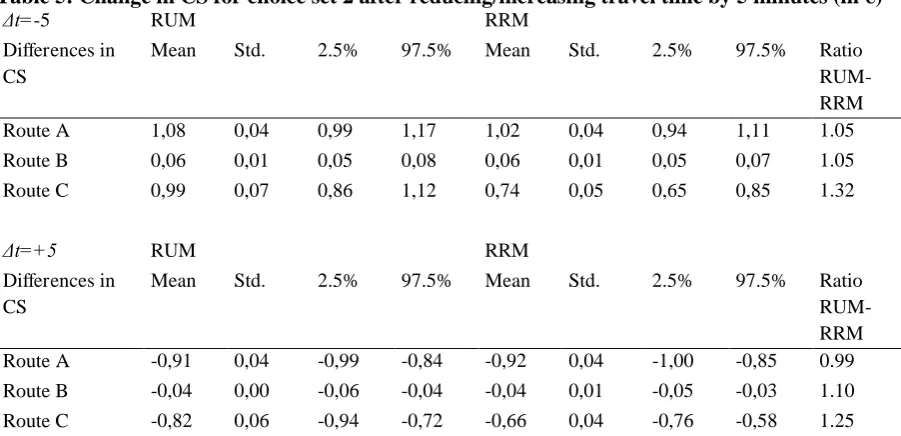
Table 5: Change in CS for choice set 2 after reducing/increasing travel time by 5 minutes (in €)
3
t=-5 RUM RRM
Differences in CS
Mean Std. 2.5% 97.5% Mean Std. 2.5% 97.5% Ratio RUM- RRM
Route A 1,08 0,04 0,99 1,17 1,02 0,04 0,94 1,11 1.05
Route B 0,06 0,01 0,05 0,08 0,06 0,01 0,05 0,07 1.05
Route C 0,99 0,07 0,86 1,12 0,74 0,05 0,65 0,85 1.32
t=+5 RUM RRM
Differences in CS
Mean Std. 2.5% 97.5% Mean Std. 2.5% 97.5% Ratio RUM- RRM Route A -0,91 0,04 -0,99 -0,84 -0,92 0,04 -1,00 -0,85 0.99
Route B -0,04 0,00 -0,06 -0,04 -0,04 0,01 -0,05 -0,03 1.10
Route C -0,82 0,06 -0,94 -0,72 -0,66 0,04 -0,76 -0,58 1.25
* Standard deviations and confidence intervals obtained using the Krinsky and Robb (1986,1990) method with 10,000 draws from the original variance covariance matrix of parameter estimates.
4
The tendency of the RRM model to put more weight on (relatively) bad attribute performances also 5
explains why we typically observe that the ratio of welfare effects of the RUM over the RRM model 6
decreases when switching from welfare gains to welfare losses. Route C in choice set one and Route B 7
in the second choice set are exceptions where we observe an increase in the ratio after deteriorating the 8
performance of the slowest alternative. 9
[image:20.595.73.524.344.562.2]20 Route C in choice set one and Route B in the second choice set are already associated with a low choice 1
probability, where the RRM provides an additional `penalty’ for bad attribute performance (see Table
2
3). Further deteriorating the performance of these two routes does not affect choice probabilities that 3
much, since both routes remain very unpopular in both RUM and RRM. However, the higher initial 4
choice probability for RUM allows for a larger welfare effect. 5
6
It can be considered remarkable that differences in welfare predictions between the RUM and RRM 7
model particularly arise in extreme scenarios. That is, RUM predicts larger welfare effects than RRM 8
when improving popular alternatives on attributes which are already outperforming those of the other 9
alternatives; RRM shows larger (negative) welfare effects when relatively popular alternatives are 10
deteriorated in the one or few attribute(s) on which they are already performing poorly. Despite the 11
subtleness – especially when applied in the context of RRM models – of the consumer surplus measure, 12
these patterns can be traced back to the properties (i.e. convexity) of the regret function and the implied 13
preference for middle-of-the-road, as opposed to extreme, attribute performance. Noteworthy is that 14
welfare implications of small changes in the attributes of compromise alternatives, which receive a 15
higher choice share in RRM models (and have been shown in the previous section to have a higher 16
existence value for regret minimisers), are comparable between the RUM and RRM model. This is a 17
result of the fact that the implications of the asymmetric regret function are less pronounced at 18
intermediate attribute levels. 19
20
As a final note, and before we discuss limitations of the proposed approach, it is worth emphasizing here 21
that the differences between RUM and RRM in terms of the value of alternatives and in the welfare 22
effects of changes in attribute values, are larger than what might be expected given the small difference 23
in model fit between the two models. This finding is in line with the more general observation (e.g., 24
Chorus et al. 2014) that despite the fact that RRM and RUM often differ hardly in terms of model fit, 25
application of the two models can lead to markedly different policy implications10.
26
10 The recently proposed muRRM model (van Cranenburgh et al. 2015) does potentially lead to larger differences
21
5. Limitations of RRM-based consumer surplus
1
Section 4 illustrated that the proposed method can be successfully applied to derive a measure of 2
(changes in) the consumer surplus (existence value) of specific alternatives within a specific choice 3
context. A direct result of using a different behavioural model is that the differences in welfare and 4
welfare effects between the linear-in-parameters-and-attributes RUM and RRM model can be 5
substantial. These differences can be traced back to differences in the core behavioural properties of the 6
RRM and RUM model. Despite these promising results, there are, however, issues regarding the 7
interpretation of the obtained RRM welfare measures, and limitations regarding the applicability of the 8
proposed method. Both will be discussed in this section. 9
10
5.1 Total surplus and aggregation bias
11
The proposed measure for changes in consumer surplus (following changes in attribute levels of an 12
alternative) that was put forward in Section 3.3 entirely focus on the existence value of alternative i. For 13
the RUM model this is inconsequential, since only the utility of alternative i is affected by changes in 14
its attribute levels. Therefore, (10) also represents the change in total consumer surplus (i.e., at the choice 15
set level) for the RUM model. In the RRM model, the attribute levels of alternative i, however, also 16
enter the regret function of the other alternatives in the choice set. Accordingly, (10) does not capture 17
changes in the existence value of the other alternatives in the choice set. Without looking into the 18
relevant equations, we already know that changes in xim bydefinition have an opposite effect on Ri and
19
Rj. Improvements in xim translate into a reduction in Ri and an increase in Rj. Hence, when CSi> 0 (i.e.,
20
when a single attribute of alternative i is improved) the proposed measure of the (change in) consumer 21
surplus for the altered alternative represents an upper bound on the change in the total surplus in the 22
choice set, since the decrease in existence value of the other alternatives is not taken into account 23
Similarly, when CSi< 0 (i.e., when a single attribute is deteriorated) a lower bound on the total welfare
24
effects in the choice set is attained. Note that the change in consumer surplus of alternative i in (10) 25
22 deteriorations implies that in absolute terms the welfare loss in the choice set will be smaller than the 1
obtained bound, i.e. closer to zero.11
2
3
McConnell (1995) derives the total surplus associated with a choice set by sequentially eliminating all 4
alternatives from the set, by means of repeatedly levying taxes in the way described before. After having 5
established the value for alternative i the price of a second (arbitrary) alternative can be gradually raised 6
to derive the consumer surplus of this particular alternative.12 The process can be repeated until all but
7
one arbitrarily selected alternatives are removed from the choice set. The inability of McConnell’s 8
method to value the only remaining alternative in the choice set introduces an aggregation bias to both 9
the RUM and RRM model. In the linear-in-income RUM model, the size of the aggregation bias can be 10
calculated using the utility of the remaining alternative divided by the marginal utility of income. This 11
is, however, impossible in the RRM model in the absence of a marginal regret of income. 12
13
5.2 Path dependency
14
Even if the value of the remaining alternative could be established in the RRM model, application of 15
McConnell’s method for total surplus in the context of RRM models remains hampered by the issue of
16
path dependency (e.g. Batley and Ibanez 2013b). For the linear-in-income RUM model the order in 17
which the alternatives are eliminated from the choice set does not affect the level of total surplus. The 18
order of elimination, however, matters for the RRM model, since increases in the price of alternative i 19
change the relative popularity of the remaining alternatives in an asymmetric fashion. This violation of 20
IIA – which, it should be noted here, is a property of the RRM model by design – induces path 21
dependency in the RRM model, i.e. a non-unique measure of the consumer surplus. 22
23
11 Note that when some attributes of alternative i are improved and others deteriorated it is impossible to set bounds
on changes in total surplus.
12 Alternative i has a zero choice probability in deriving this subsequent consumer surplus, since it has been made
23 Path dependency thereby also precludes the identification of welfare effects of simultaneous changes in 1
the attribute levels of multiple alternatives in the choice set. Indeed, the value of alternative i changes 2
due to changes in its own attributes as well as in those of a competing alternative z. We can define a 3
change in value for the distinct alternatives i and z using (10). The implications on the joint surplus for 4
i and z, however, varies with the adopted tax path from (0,0) to ( , . Furthermore, the opposite 5
directional effect of changes in i (or z) on the regret of the other alternatives in the choice sets precludes 6
setting bounds on the overall implications of the change on the total surplus of the choice set. 7
8
Despite the limitations discussed in this section, we believe that the proposed measure constitutes a step 9
forward for RRM-based welfare analysis as it allows researchers to compute the existence value of 10
specific alternatives and the impact of changes in the alternative’s attributes on its existence value. 11
Furthermore, the proposed measure provides insight into the impact on total consumer surplus (i.e., the 12
value of the full choice set) of changes in the attributes of a specific alternative. Although the latter 13
measure only provides a bound on the maximum welfare implications of such a change, this is much 14
more informative than having no information at all regarding the resulting welfare implications. 15
16
6. Conclusions and future research
17
Since its introduction, the Random Regret Minimisation model has received significant attention in the 18
field of choice modelling and has been applied to a broad range of stated choice and revealed preference 19
datasets (see Chorus et al. 2014 for an overview). Due to its empirical nature and its behavioural, rather 20
than axiomatic underpinning, the model’s capacity to conduct welfare analysis is yet to be determined,
21
but very likely to be considerably more limited than that of conventional AIRUM models. At first sight, 22
the absence of a marginal regret of income even precludes a meaningful RRM-based welfare analysis. 23
In this paper however, we show that observed behavioural responses to price changes can be applied to 24
approximate certain specific Marshallian measures of consumer surplus. 25
24 The proposed method interprets the RRM-based choice probability ‘as if’ it represents a probabilistic 1
demand function. It should, however, be noted that in contrast to RUM models, the RRM-based indirect 2
utility function has no direct utility function counterpart which adheres to the principles as set out by 3
Batley and Ibanez (2013a). Nevertheless, the choice probability is the best and most well-behaved 4
approximation available of how consumers respond to price and quality changes in a discrete choice 5
context. Following the tradition in microeconomics, measuring the area underneath the probabilistic 6
demand function up to a choke price assigns an existence value to an alternative in the context of a 7
particular choice set. The capability of the RRM model to account for choice set composition effects is 8
clearly reflected in the predicted consumer surplus measures and their differences from RUM-9
counterparts. For example, the RRM model assigns a higher value to so-called compromise alternatives 10
as it favours intermediate – as opposed to extreme – performance on the different attributes 11
characterizing an alternative, relative to the attributes of competing alternatives. Changes in the value 12
of an alternative as a result of changes in its attribute levels can also be valued using the same method, 13
where the method becomes simpler when a price change is considered. We find that differences between 14
the welfare effects predicted by the RUM and RRM model are largest when alternatives are improved 15
on attributes on which they are already performing well. These findings are again in line with differences 16
in behavioural premises underlying RUM and RRM models, in the sense that the convexity of the RRM 17
model tempers such welfare gains, compared to the RUM model. In most other cases, the differences 18
between the RUM and RRM welfare effects are more comparable, but also these more subtle differences 19
can still be traced back to the core properties of the RRM model. 20
21
We discuss in what ways the developed welfare measure is incomplete. Indeed, it only focuses on the 22
change in surplus for the altered alternative and not the change in total surplus; aggregation bias and 23
path dependency prevent the quantification of these overall welfare implications for the entire choice 24
set, i.e. the net welfare effect. When unidirectional changes in the attribute levels are introduced, we are 25
however able to set an upper bound on the resulting welfare gains and losses in the entire choice set. 26
Note that these bounds differ from the theoretical bounds discussed by Batley and Dekker (2017); Morey 27
25 these bounds arise because the actual regret of unaltered alternatives is affected by improving a 1
particular environmental alternative. The latter could potentially prevent a priori knowledge on the 2
direction of the net welfare effect. The issue is closely related to the non-monotonicity of the expected 3
minimum regret in the RRM model (Chorus 2012). A second limitation of the method is the 4
impossibility to value changes in the attributes of multiple alternatives as non-unique welfare estimates 5
will in that case be obtained due to path dependency. Nevertheless, this paper provides researchers a 6
tool to quantify certain welfare implications based on the RRM model. These limitations, however, 7
significantly limit the application of the RRM model in combination with social welfare measurement, 8
leaving the researcher with the inevitable trade-off between behavioural relevance and economic theory 9
based social welfare analysis. 10
11
Naturally, these limitations call for future research and ultimately a movement towards Hicksian (or 12
compensated) welfare measures which are not hampered by path dependency. The simple solution is to 13
adhere to the AIRUM specification and only allow for context dependency in the non-price attributes. 14
We provide a little thought experiment here when one wishes to keep treating prices in a RRM fashion. 15
Hicksian measures require an individual to be indifferent before and after a change in attribute levels. 16
Section 2 already established that income compensation is not feasible in the context of the RRM model. 17
Price compensation may, however, be an alternative measure of compensation. One could ask the 18
question, what is the minimum amount of price compensation required to bring the individual back to 19
his old regret (utility) level? Essential in the context of random regret (utility) are the implications of 20
switching behaviour (e.g. Karlström and Morey 2001). As such it may not matter of which alternative 21
the regret is reduced to the minimum level of regret experienced in the original choice set. Particularly 22
the non-linearity of regret with respect to price (and attributes) may cause that price changes in other 23
alternatives are more effective to bring regret back to its original level at a lower cost. The relevant 24
question therefore becomes: what is the minimum amount of price compensation required and on which 25
alternative to bring the minimum regret in the choice set back to its original level? This requires either 26
extending the method proposed by Karlström and Morey (2001) or applying McFadden’s (1995)
27
26 properties of such a measure of compensating variation would need to be established. Violations of the 1
conditions specified in Batley and Ibanez (2013a) are foreseen, such as symmetry, but some of these 2
also extend to the framework of utility functions which are non-linear in income. 3
4
Finally, our analysis has been at the level of the individual, not the representative consumer. A particular 5
reason for this is that the described preference relations do not take the well-known Gorman polar form. 6
This requires judgements with respect to aggregation of individual welfare effects for the purpose of 7
economic appraisal. Our empirical examples assume preferences are constant across individuals, but it 8
is not uncommon that preferences vary across income groups (or other socio-economic characteristics). 9
In both the RUM and RRM model, heterogeneity in preferences has implications for the implemented 10
social welfare function. The welfare function may be corrected for such effects by means of income 11
adjusted weights (e.g. UK Treasury 2011). 12
13
Acknowledgements
14
The authors gratefully acknowledge support from the Netherlands Organisation for Scientific Research 15
(NWO), in the form of VIDI-grant 016-125-305. 16
17
References
18
Adamowicz, W. L., Glenk, K., & Meyerhoff, J. (2014). Choice modelling research in environmental 19
and resource economics. Chapter 27, pages 661-674, in Hess, S. & Daly, A. (Eds.) Handbook of Choice 20
Modelling, Edward Elgar, Cheltenham, UK. 21
22
Batley R. 2016. Income effects, cost damping and the value of time: theoretical properties embedded 23
within practical travel choice models. Transportation, in press. doi:10.1007/s11116-016-9744-0 24
25
Batley R. and Dekker, T. 2017. The intuition behind income effects of price changes in discrete choice 26
models, and a simple method for measuring the compensating variation. ITS Working Paper, University 27
of Leeds. 28
27 Batley R. and Ibanez, N. 2013a. Applied welfare economics with discrete choice models: implications 1
for empirical specification. In: Choice modelling: the state of the art and the state of practice, Eds: Hess, 2
S. and Daly, A., Edward Elgar, Cheltenham, UK. 3
4
Batley R. and Ibanez, N. 2013b. On the path independence conditions for discrete-continuous demand. 5
Journal of Choice Modelling, 7, 13-23. 6
7
Ben-Akiva M. and Lerman, S. 1985. Discrete choice analysis: theory and application to travel demand. 8
The MIT Press. 9
10
Boeri, M., Longo, A., Doherty, E., & Hynes, S. (2012). Site choices in recreational demand: a matter of 11
utility maximization or regret minimization?. Journal of Environmental Economics and Policy, 1(1), 12
32-47. 13
14
Chorus, C.G., 2010. A new model of Random Regret Minimization. European Journal of Transport and 15
Infrastructure Research, 10(2), 181-196. 16
17
Chorus, C.G. 2012. Logsums for utility maximizers and regret-minimizers, and their relation with 18
desirability and satisfaction. Transportation Research Part A: Policy and Practice, 46(7), 1003-1012. 19
20
Chorus, C.G. and Bierlaire, M., 2013. An empirical comparison of travel choice models that capture 21
preferences for compromise alternatives. Transportation, 40, 549-562. 22
23
Chorus, C.G. van Cranenburgh, S. and Dekker, T., 2014. Random regret minimization for consumer 24
choice research: Assessment of empirical evidence. Journal of Business Research, 67, 2428-2436. 25
26
Cochrane, R.A. 1975. A possible economic basis for the gravity model. Journal of Transport Economics 27
and Policy, 9(1), 34-49. 28
29
Dagsvik, J.K. and Karlström, A., 2005. Compensating variation and Hicksian choice probabilities in 30
random utility models that are non-linear in income. Review of Economic Studies, 72(1), 57-76. 31
32
Deaton, A. and Muellbauer, J. 1980. Economics and Consumer behaviour. Cambridge University Press. 33
34
De Jong, G., Daly, A., Pieters, M. and van der Hoorn, T. 2007. The logsum as an evaluation measure: 35
review of the literature and new results. Transportation Research Part A: Policy and Practice, 41(9), 36
874-889. 37
38
Dekker, T., 2014. Indifference based Value of Time measures for Random Regret Minimisation models, 39
Journal of Choice Modelling, 12, 10-20. 40
41
De Palma, A. and Kilani, K. 2011. Transition choice probabilities and welfare analysis in additive 42
random utility models. Economic Theory, 46(3), 427-454. 43
44
EconometricSoftware (2012). NLOGIT Version 5.0 Reference Guide. (Plainview, NY, USA). 45
46
Edwards, W. 1961. Behavioral decision theory. Annual review of psychology, 12(1), 473-498. 47
28 Einhorn, H. J., and Hogarth, R. M. 1981. Behavioral decision theory: Processes of judgment and choice. 1
Journal of Accounting Research, 1-31. 2
3
Guevara, C. A. and Fukushi, M. 2016. Modeling the decoy effect with context-RUM Models: 4
Diagrammatic analysis and empirical evidence from route choice SP and mode choice RP case studies. 5
Transportation Research Part B: Methodological, 93, 318-337. 6
7
Hanemann, M., 1984. Welfare evaluations in contingent valuation experiments with discrete responses. 8
American Journal of Agricultural Economics, 66(3), 332-341. 9
10
Harris, A.J. and Tanner, J.C. 1974. Transport demand models based on personal characteristics. 11
Transport and Road Research Laboratory Supplementary Report 65UC, Berkshire; Reprinted in the 12
Symposium Proceedings of the Sixth International Symposium on Transportation and Traffic Theory, 13
Sydney Australia. 14
15
Hensher, D. A., Greene, W. H. and Rose, J. M. 2015. Applied choice analysis: a primer. (Cambridge: 16
Cambridge University Press), Second Edition. 17
18
Herriges, J.A. and Kling, C.L. 1999. Nonlinear income effects in random utility models, The Review of 19
Economics and Statistics, 81, 62-72. 20
21
Hess, S., Polak, J., Daly, A. and Hyman, G. 2007. Flexible substitution patterns in models of mode and 22
time of day choice: new evidence from the UK and the Netherlands. Transportation, 34(2), 213-238. 23
24
Jara-Diaz, S. and Videla, J. 1989. Detection of income effect in mode choice: theory and application. 25
Transportation Research Part B: methodological, 23(6), 393-400. 26
27
Karlström, A. and Morey, E.R. 2001. Calculating the exact compensating variation in logit and nested-28
logit models with income effects: theory, intuition, implementation and application. Paper presented at 29
the meeting of the American Economic Association, New Orleans, January 2001. 30
31
Krinsky I. and Robb A. L., 1986. On Approximating the Statistical Properties of Elasticities. The Review 32
of Economics and Statistics, 68(4), 715-719. 33
34
Krinsky I. and Robb A. L. 1990. On Approximating the Statistical Properties of Elasticities: A 35
Correction, The Review of Economics and Statistics, 72(1), 189-190. 36
37
Leong, W., Hensher, D.A. 2015. Contrasts of Relative Advantage Maximisation with Random Utility 38
Maximisation and Regret Minimisation? Journal of Transport Economics and Policy, 49(1), 167-186. 39
40
Loomes, G. and Sugden, R. 1982. Regret theory: an alternative theory of choice under uncertainty. The 41
Economic Journal, 92(368), 805-824. 42
43
McConnell, K.E., 1995. Consumer surplus for discrete choice models. Journal of Environmental 44
Economics and Management, 29(3), 263-270. 45
46
McFadden, D., 1981. Econometric models of probabilistic choice. In: Structural analysis of discrete 47
29 McFadden, D., 1995. Computing willingness-to-pay in random utility models. Department of 1
Economics, University of California, Berkeley. 2
3
Morey, E. 1994. What is consumer surplus per day of use, when is it a constant independent of the 4
number of days use and what does it tell us about consumer surplus? Journal of Environmental 5
Economics and Management, 26, 257-270. 6
7
Morkbak, M.R., Christensen, T. and Gyrd-Hansen, D. 2010. Choke price bias in choice experiments. 8
Environmental and Resource Economics, 45(4), 537-551. 9
10
Neuberger, H. 1971. User benefit in the evaluation of transport and land use plans. Journal of Transport 11
Economics and Policy, 5, 52-75. 12
13
Simonson, I. and Tversky, A. 1992. Choice in context: tradeoff contrast and extremeness aversion. 14
Journal of Marketing Research, 29(3), 281-295. 15
16
Slovic, P., Fischhoff, B., and Lichtenstein, S. 1977. Behavioral decision theory. Annual review of 17
psychology, 28(1), 1-39. 18
19
Small, K.A. and Rosen, H.S. 1981. Applied welfare economics with discrete choice models. 20
Econometrica, 105-130. 21
22
Street, D., Burgess, L. and Louviere, J. 2005. Quick and easy choice sets: constructing optimal and 23
nearly optimal stated choice experiments. International Journal of Research in Marketing, 22, 459-470. 24
25
Thiene, M., Boeri, M., & Chorus, C. G. (2012). Random regret minimization: exploration of a new 26
choice model for environmental and resource economics. Environmental and resource economics, 27
51(3), 413-429. 28
29
Tversky, A. and Kahneman, D. 1991. Loss aversion in riskless choice: A reference-dependent model. 30
The quarterly journal of economics, 106(4), 1039-1061. 31
32
Train, K.E., 2009. Discrete choice with simulation. Cambridge University Press, New York. 33
34
UK Treasury 2011. The Green Book: Appraisal and evaluation in central government. 35
https://www.gov.uk/government/uploads/system/uploads/attachment_data/file/220541/green_book_co
36
mplete.pdf 37
38
Van Cranenburgh, S. Guevara, C.A. and Chorus, C.G. 2015. New insights on random regret 39
minimisation models. Transportation Research Part A: Policy and Practice, 74, 91-109. 40
41
Vermunt, J. K. and Magidson, J. (2014). Upgrade manual for Latent GOLD Choice 5.0. (Belmont, MA 42
, USA). 43
44
Williams, H.C.W.L. 1977. On the formation of travel demand models and economic evaluation 45
measures of user benefit. Environment and Planning A, 9, 285-344. 46