cache-related pre-emption delays: : integrated analysis and evaluation
.
White Rose Research Online URL for this paper:
http://eprints.whiterose.ac.uk/112023/
Version: Published Version
Article:
Bril, Reinder, Altmeyer, Sebastian, van den Heuvel, Martijn et al. (2 more authors) (2017)
Fixed priority scheduling with pre-emption thresholds and cache-related pre-emption
delays: : integrated analysis and evaluation. Real-Time Systems. pp. 1-64. ISSN
1573-1383
https://doi.org/10.1007/s11241-016-9266-z
[email protected] https://eprints.whiterose.ac.uk/
Reuse
This article is distributed under the terms of the Creative Commons Attribution (CC BY) licence. This licence allows you to distribute, remix, tweak, and build upon the work, even commercially, as long as you credit the authors for the original work. More information and the full terms of the licence here:
https://creativecommons.org/licenses/
Takedown
If you consider content in White Rose Research Online to be in breach of UK law, please notify us by
DOI 10.1007/s11241-016-9266-z
Fixed priority scheduling with pre-emption thresholds
and cache-related pre-emption delays: integrated
analysis and evaluation
Reinder J. Bril1,2 · Sebastian Altmeyer3 ·
Martijn M. H. P. van den Heuvel2 · Robert I. Davis4 ·
Moris Behnam1
© The Author(s) 2017. This article is published with open access at Springerlink.com
Abstract Commercial off-the-shelf programmable platforms for real-time systems typically contain a cache to bridge the gap between the processor speed and main memory speed. Because cache-related pre-emption delays (CRPD) can have a signif-icant influence on the computation times of tasks, CRPD have been integrated in the response time analysis for fixed-priority pre-emptive scheduling (FPPS). This paper presents CRPD aware response-time analysis of sporadic tasks with arbitrary dead-lines for fixed-priority pre-emption threshold scheduling (FPTS), generalizing earlier work. The analysis is complemented by an optimal (pre-emption) threshold assign-ment algorithm, assuming the priorities of tasks are given. We further improve upon these results by presenting an algorithm that searches for a layout of tasks in memory that makes a task set schedulable. The paper includes an extensive comparative eval-uation of the schedulability ratios of FPPS and FPTS, taking CRPD into account. The practical relevance of our work stems from FPTS support in AUTOSAR, a standard-ized development model for the automotive industry. [(This paper forms an extended version of Bril et al. (in Proceedings of 35th IEEE real-time systems symposium (RTSS),2014). The main extensions are described in Sect.1.2.]
Keywords Fixed-priority pre-emptive scheduling·Fixed-priority scheduling with pre-emption thresholds·Cache-related pre-emption delay·Response-time analysis
B
Reinder J. Bril [email protected]1 Mälardalen University (MDH), Västerås, Sweden
1 Introduction
1.1 Background and motivation
For cost-effectiveness reasons, it is preferred to use commercial off-the-shelf (COTS) programmable platforms for real-time embedded systems rather than dedicated, application-domain specific platforms. These COTS platforms typically contain a cache to bridge the gap between the processor speed and main memory speed and to reduce the number of conflicts with other devices on the system bus. Unfortunately, caches give rise to additional delays upon pre-emptions, because pre-emptions may lead to cache flushes and reloads of blocks that are replaced. These cache-related pre-emption delays (CRPDs) can significantly increase the computation times of tasks, i.e., literature has reported inflated computation times of up to 50% (Pellizzoni and Caccamo2007. In order to account for the impact of the CRPD on the timeliness of a task system, CRPD has therefore been integrated into the schedulability analysis of tasks (Busquets-Mataix et al.1996; Lee et al.1998; Staschulat et al.2005; Ramaprasad and Mueller2006; Altmeyer et al.2012).
In real-time embedded systems, such as embedded vehicle control, fixed-priority pre-emptive scheduling (FPPS) is widely used. The majority of the commercial real-time operating systems (RTOSes) supports FPPS and makes use of corresponding timing-analysis tools. FPPS is inherently fully pre-emptive, which causes at least two types of pre-emption costs when using COTS hardware: spatial costs for saving and restoring the context of all tasks in memory and contention delays such as CRPD when cache blocks need to be reloaded. With FPPS these run-time overheads cannot be resolved analytically. An important disadvantage of FPPS therefore remains that arbitrary pre-emptions during execution may lead to inefficient memory use and high run-time overheads (Gai et al.2001; Ghattas and Dean2007).
In order to overcome these inefficiencies, some RTOS manufacturers were inclined to use two static priorities per task (Carbone2013; Wang and Saksena1999): one base priority is applied at task dispatching (sometimes also referred to as a task’sdispatching priority) and a second priority is applied once a task is selected for execution until its completion (referred to as a task’spre-emption threshold). This scheme of fixed-priority scheduling with pre-emptions thresholds (FPTS) has been shown to greatly reduce the memory footprint of concurrent task systems (Gai et al.2001) and reduce the average case response times of tasks (Ghattas and Dean2007). Currently, FPTS is therefore already adopted by industry.
To the best of our knowledge, however, the integration of CRPD in the schedulability analysis of FPTS has not been considered. The limited pre-emptive nature of FPTS gives rise to specific challenges when integrating CRPD in the analysis, in particular to prevent over-estimations of CRPD. For example, not all tasks contributing to the worst-case response time of a task can actually pre-empt the execution of a job of that task, unlike with FPPS, as illustrated by a non-pre-emptive task. Next, there is no optimal (pre-emption) threshold assignment (OTA) algorithm available for FPTS taking CRPD into account, not to mention an algorithm that minimizes CRPD. Finally, existing comparisons between FPPS and FPTS, e.g. Buttazzo et al. (2013), do not consider CRPD.
1.2 Contributions
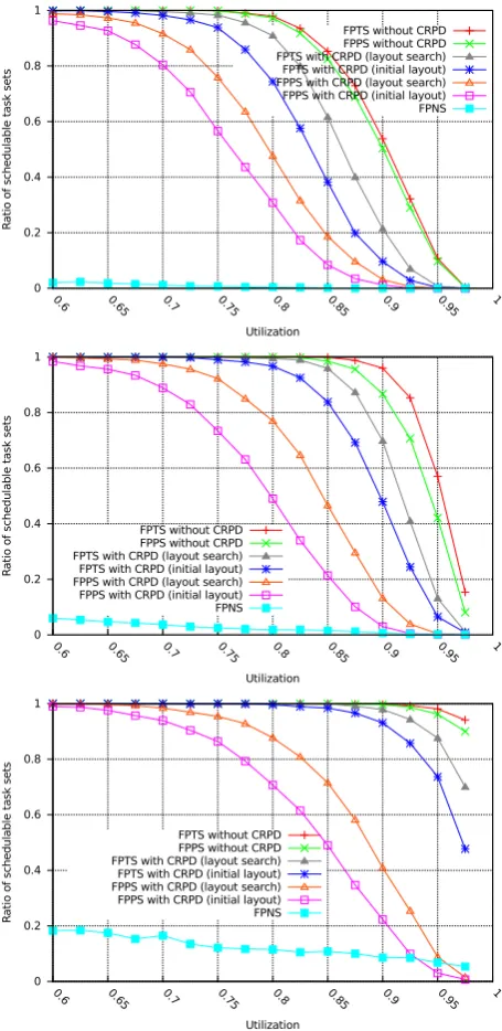
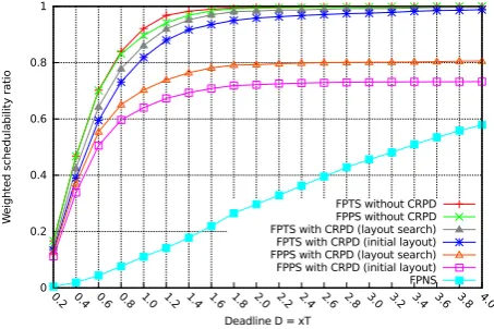
This paper presents four main contributions. Firstly, it provides worst-case response-time analysis of sporadic tasks with arbitrary deadlines for FPTS with CRPD, generalizing the work in Altmeyer et al. (2012) from FPPS to FPTS and from con-strained deadlines to arbitrary deadlines. Secondly, it provides and proves an OTA algorithm for FPTS with CRPD. Thirdly, it presents a schedulable task-layout search (STLS) algorithm that searches for a layout of tasks in memory that makes a task set schedulable. The algorithm generalizes the one in Lunniss et al. (2012) from FPPS to FPTS by exploring memory layouts and applying the OTA algorithm to them. In this way, reloads of memory blocks into the cache result in minimal CRPD for the consid-ered memory layout. Finally, this paper presents an extensive comparative evaluation of the schedulability ratios of FPPS and FPTS with and without CRPD. The evaluation is based on three orthogonal dimensions, i.e. (i) theCRPD approachapplied in the analysis, (ii) thedeadline type, being constrained, implicit, and arbitrary deadlines, and (iii) thememory layout, and seven main experiments in which task-set parameters and cache related parameters are varied. In addition, the effectiveness of the STLS algorithm is evaluated.
1.2.1 Extended version
Compared to Bril et al. (2014), this extended version has the following two major contributions. Firstly, it presents a generalized algorithm to improve the layout of tasks in memory (Sect.10). Secondly, it presents a major extension of the comparative evaluation (Sect. 11). In particular, we added two orthogonal dimensions, i.e. the CRPD approachand thedeadline type, and two experiments, i.e. the evaluation of the STLS algorithm (Sect.11.2.2) and cache reuse (Sect.11.4.3).
1.3 Outline
The remainder of this paper is organized as follows. Section2presents related work. Section3presents our scheduling model for FPTS and CRPD. Section4recapitulates analysis for FPTS without CRPD and analysis for FPPS with CRPD. Sections5–8
in Bril et al. (2014)]. The analysis is split into the following sections: Sect.5addresses the main challenges, Sect.6focusses on pre-empting tasks, Sect.7on the pre-empted tasks and Sect.8combines pre-empting and pre-empted tasks.
Next, Sect.9presents our Optimal Threshold Assignment (OTA) algorithm. Sec-tion10presents our STLS algorithm which aims at further decreasing the CRPD by improving the layout of the memory blocks of tasks. Section11evaluates the perfor-mance of FPPS and FPTS in the presence of CRPD. Finally, Sect.12concludes this paper. A complementary appendix contains all graphs of the comparative evaluation.
2 Related work
In this section, we first present an overview of scheduling schemes (including FPTS) that may reduce the number of pre-emptions and their related costs in concurrent real-time task systems. Secondly, we look at related works that investigated techniques for dealing with CRPDs in pre-emptive systems.
2.1 Limited pre-emptive scheduling
Limited pre-emptive scheduling schemes received a lot of attention from academia in the last decade. In particular, fixed-priority scheduling with deferred pre-emption (FPDS) (Burns 1994; Bril et al. 2009; Davis and Bertogna 2012), also called co-operative scheduling, and fixed-priority scheduling with pre-emption thresholds (FPTS) (Wang and Saksena1999; Saksena and Wang2000; Regehr2002; Keskin et al.
2010) are considered viable alternatives between the extremes of fully pre-emptive and non-emptive scheduling. Compared to fully emptive scheduling, limited pre-emptive schemes can (i) reduce memory requirements (Saksena and Wang2000; Gai et al.2001; Davis et al.2000) and (ii) reduce the cost of arbitrary pre-emptions (Burns
1994; Bril et al.2009; Bertogna et al.2011b). In addition, compared to both FPPS and non-pre-emptive scheduling, these schemes may significantly improve the schedula-bility of a task set (Bril et al.2009; Saksena and Wang2000; Bertogna et al.2011a; Davis and Bertogna2012).
Although FPDS also outperforms FPTS from a theoretical perspective (Buttazzo et al.2013), applying FPDS in practice is still a challenge, because pre-emption points have to be explicitly added in the code. Bertogna et al. (2011b) presented a model based on constant pre-emption costs in order to place pre-emption points in the tasks’ code appropriately. Recently, Cavicchio et al. (2015) have further extended this work by placing pre-emption points after computing and optimizing the CRPDs of a task. However, these works assume a linear flow of the code blocks of tasks. In our current work on FPTS we refrain from any assumption on the structure of the tasks’ code.
2.2 Cache-related pre-emption delays (CRPDs)
There are different techniques to deal with CRPDs. If the total number of memory blocks of the tasks in a system exceeds the cache size, then this may obviously lead to CRPDs due to reloads of blocks from memory to the cache. However, even if all memory blocks fit in the cache simultaneously, there are scenarios in which some memory blocks that are occupied by the tasks may be mapped to the same cache block. Since the mapping of memory to cache is often statically prescribed by the hardware (Patterson and Hennessy2014), a proper memory layout of the tasks is important even when the total number of occupied memory blocks fits into the cache. Gebhard and Altmeyer (2007) and Lunniss et al. (2012) therefore tried to optimize the CRPDs by changing the layout of tasks in memory, subject to a static mapping of memory blocks to cache blocks. In our paper, we build upon the earlier work for FPPS by Lunniss et al. (2012) and we generalize their approach to FPTS.
are relatively high compared to the computation times. However, they observed that the advantage of cache partitioning is often negligible when the memory layout of tasks is improved, so that memory blocks are loaded in the cache with less overlap. Moreover, cache partitioning is not very suitable for tasks with lower locality of mem-ory accesses and higher amounts of computation, i.e. when the pre-emption costs are small compared to the computation times.
Wang et al. (2015) extended the applicability of cache partitioning to larger task sets with the help of FPTS. They created mutual non-pre-emptive task groups, so that tasks of the same group can together use a larger cache partition. However, we expect that the scalability of their approach is limited, because for large task sets, with lower locality of memory accesses and higher amounts of computation, FPTS will suffer from the same drawbacks as FPPS. The elimination of CRPDs between tasks may then not compensate for the performance degradation in the computation times of tasks. In the current paper, we therefore follow the line of reasoning by Altmeyer et al. (2014) and we complement our assignment of pre-emption thresholds with an algorithm for improving the memory layout of tasks.
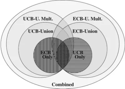
The CRPDs of tasks can be analysed based on the concepts ofevicting cache blocks (ECBs) anduseful cache blocks(UCBs) (Lee et al.1998; Altmeyer and Maiza2011). A cache block that may be accessed by a task is termed an ECB, as it may overwrite the content of that cache block. A cache block that may be (re-) used at multiple program points without being evicted by the task itself is termed a UCB. The set of UCBs and ECBs of tasks can be analyzed with, for example, a prototype version of AbsInt’saiT Timing Analyzer for ARM (Ferdinand and Heckmann2004). This type of analysis using ECBs and UCBs applies to direct-mapped caches with a write-through policy and to set-associative caches with a least-recently used (LRU) replacement policy and a write-through policy (Altmeyer et al.2012). The concepts of ECBs and UCBs cannot be applied to set-associative caches with a first-in-first-out (FIFO) or a pseudo-LRU (PLRU) replacement policy, as shown in Burguière et al. (2009).
The integration of CRPD in the schedulability analysis of tasks has been addressed for FPPS with a focus on the pre-empting tasks (Busquets-Mataix et al. 1996; Tomiyama and Dutt2000), thepre-empted tasks(Lee et al.1998), and by considering both thepre-empting and pre-empted tasks(Staschulat et al.2005; Tan and Mooney
2007; Altmeyer et al.2012). Figure1gives an overview of the various approaches and their relation. When focussing on the pre-empting tasks, only the ECBs of a task
Fig. 1 Venn diagram showing the relationship between the different approaches for computing CRPDs (as presented by Altmeyer et al.2012)
Combined ECB
Only
UCB-Union
UCB Only ECB-Union UCB-U. Mult. ECB-U. Mult.
(2012). In the current paper we extend the most effective approaches to FPTS, i.e., the UCB/ECB-Union Multiset approaches.
3 Models and notation
This section presents the models and notation that we use throughout this paper. We start with a basic, continuous scheduling model for FPPS, i.e., we assume time to be taken from the real domain (R), similar to, e.g., Koymans (1990), Bril et al. (2009) and Bertogna et al. (2011a). We subsequently refine this basic model for FPTS (Wang and Saksena1999). Next, we introduce a basic memory model and a model for cache-related pre-emption costs. The section is concluded with remarks.
3.1 Basic model for FPPS
We assume a single processor and a set T of n independent sporadic tasks
τ1, τ2, . . . , τn, with unique prioritiesπ1, π2, . . . , πn. At any moment in time, the pro-cessor is used to execute the highest priority task that has work pending. For notational convenience, we assume that (i) tasks are given in order of decreasing priorities, i.e.
τ1has the highest andτnthe lowest priority, and (ii) a higher priority is represented by a higher value, i.e.π1> π2> . . . > πn. We use hp(π )(and lp(π )) to denote the set of tasks with priorities higher than (lower than)π. Similarly, we use hep(π )(and lep(π )) to denote the set of tasks with priorities higher (lower) than or equal toπ.
Each taskτi is characterized by aminimum inter-activation time Ti ∈R+, a
worst-case computation time Ci ∈ R+, and a (relative) deadline Di ∈ R+. We assume that the constant pre-emption costs, such as context switches and pipeline flushes, are subsumed into the worst-case computation times. We feature arbitrary deadlines, i.e. the deadline Di may be smaller than, equal to, or larger than the periodTi. The
[image:8.439.188.388.60.202.2]Table 1 Notations for various
sets of indices of tasks Classic notations for FPPS Additional notations for FPTS
hep(π )def= {h|πh≥π} het(π )def= {h|θh≥π}
lp(π )def= {ℓ|π > πℓ} lt(π )def= {ℓ|π > θℓ} hp(π )def= {h|πh> π} b(i)
def
= lp(πi)\lt(πi)
lep(π )def= {ℓ|π≥πℓ}
We also adopt standard basic assumptions (Liu and Layland1973), i.e. tasks do not suspend themselves and a job of a task does not start before its previous job is completed.
For notational convenience, we introduce Ej(t) =
t/Tj
and E∗j(t) =
1+t/Tj
to represent the maximum number of activations ofτj in an interval
[x,x+t)and[x,x+t], respectively, where both intervals have a lengtht.
3.2 Refined model for FPTS
In FPTS, each taskτihas apre-emption thresholdθi, whereπ1≥θi ≥πi. Whenτiis executing, it can only be pre-empted by tasks with a priority higher thanθi. Note that we have FPPS and FPNS as special cases when∀1≤i≤nθi =πi and∀1≤i≤nθi =π1,
respectively.
We use het(π )(and lt(π )) to denote the set of tasks with thresholds higher than or equal to (lower than)π. Finally, we useb(i)to denote the set of tasks that may block
τi due to their pre-emption threshold assignment. An overview of notations for sets of tasks is given in Table1. Note that for FPPS hep(π )=het(π ),lp(π )=lt(π ), and b(i)= ∅.
3.3 A memory model
We consider two types of memory, (main) memory and cache (memory). Memory and cache are assumed to contain (memory) blocks of a fixed size, where memory contains NMblocks and cacheNCblocks, and typicallyNM ≫NC. Memory blocks and cache blocks are numbered from 0 untilNM−1 and from 0 toNC−1, respectively. Similar to Altmeyer et al. (2012), we assume direct-mapped caches (Patterson and Hennessy
2014), i.e. a memory block is mapped to exactly one cache block, with a write-through policy. A typical mapping schemeMapM2C for direct-mapped caches and systems without virtual memory is that memory blockmis mapped to cache block
MapM2C(m)=mmodNC. (1)
The cache utilization of a taskτi is given by UiC = |MBi|/NC, where|MBi| denotes the cardinality of the set MBi. The cache utilization of an individual task can therefore be larger than one, i.e. when|MBi|>NC. Thecache utilization UCof the set of tasksT is given byUC=
1≤i≤nUiC.
The set of cache blocks of taskτi is determined by MBi andMapM2C.
3.4 A model for cache-related pre-emption costs
Similar to Altmeyer et al. (2012), we use also the concepts ofevicting cache blocks (ECBs) and useful cache blocks(UCBs) in order to analyze CRPDs. The ECBs of a taskτi are denoted by the set ECBi; the UCBs of a taskτi are denoted by the set UCBi. Just like MBi, these sets are also represented as sets of natural numbers. By definition, the set UCBiis a subset of the set ECBi, i.e. UCBi ⊆ECBi. The set ECBi is determined by
ECBi = m∈MBi
MapM2C(m). (2)
Example1shows the relation between the ECBs of a task (ECBi), the UCBs of a task (UCBi) and the BRT.
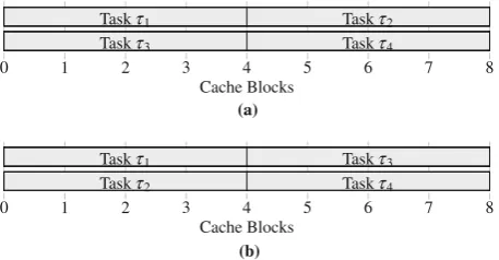
Example 1 We assume a direct-mapped cache with 4 cache blocks and two tasksτ1
andτ2. The memory blocks ofτ1map to cache blocks 0,1 and 2. Onlyτ1’s memory
block mapping to cache block 1 is useful, i.e. ECB1 = {0,1,2}and UCB1 = {1}.
The memory blocks ofτ2map to cache blocks 1,2, and 3 and all three are useful, i.e.
ECB2= {1,2,3}and UCB2= {1,2,3}. The cache-related pre-emption cost of task
τ1pre-empting taskτ2is thus given as follows:
|ECB1∩UCB2| ·BRT= |{1,2}| ·BRT=2·BRT.
Whether or not all memory blocks of a taskτi can be mapped on different cache blocks depends on the memory size|MBi|of τi and the size NC of the cache. As described in Altmeyer et al. (2014) and Wang et al. (2015), the worst-case computation time of a task depends on the size of the cache. Whereas the worst-case computation Ci of taskτi is fixed when|MBi| ≤NC, it may increase when|MBi|becomes larger than NCdue toself-eviction, i.e.τi may evict some of its own cache blocks. In the remainder, we will assume that the costs of self-evictions, which are also referred to as intra-task CRPDs, are subsumed into the worst-case computation times.
3.5 Concluding remarks
4 Recap of response time analysis for FPPS and FPTS
This section starts with a recapitulation of the exact schedulability analysis for FPTS, as presented in Keskin et al. (2010). Next, that analysis is specialized for FPPS with constrained deadlines, i.e. for cases withDi ≤Ti, and extended with CRPD (Altmeyer et al.2012).
4.1 FPTS with arbitrary deadlines (without CRPD)
A set T of tasks is schedulable if and only if for every task τi ∈ T its worst-case
response timeRiis at most equal to its deadlineDi, i.e.∀1≤i≤nRi ≤ Di. To determine
Ri, we need to consider the worst-case response times of all jobs in a so-called level-i active period (Bril et al.2009). The worst-case lengthLi of that period is given by the smallest positive solution of
Li =Bi+
∀j∈hep(πi)
Ej(Li)·Cj, (3)
whereBi denotes the worst-case blocking of taskτi, given by
Bi =max
0, max
∀b∈b(i)Cb
. (4)
Li can be found by fixed point iteration that is guaranteed to terminate for alli when
U <1 (Bril et al.2009).
As mentioned above, when a taskτiis executing, it can only be pre-empted by tasks
τj with j ∈ hp(θi). In the worst-case response time analysis, we therefore consider both the start-time and the finishing time of a job of a task. For a jobkof τi, with 0 ≤k < Ei(Li), the worst-case start timeSi,kand worst-case finalization time Fi,k are given by
Si,k= ⎧ ⎪ ⎨ ⎪ ⎩
Bi +kCi + ∀j∈hp(πi)
Ej(Si,k)·Cj ifBi >0
kCi+ ∀j∈hp(πi)
E∗j(Si,k)·Cj ifBi =0 (5)
and
Fi,k =Si,k+Ci+ ⎧ ⎪ ⎨ ⎪ ⎩
∀j∈hp(θi)
Ej(Fi,k)−Ej(Si,k)
·Cj ifBi >0
∀j∈hp(θi)
Ej(Fi,k)−E∗j(Si,k)
·Cj ifBi =0
. (6)
Later in this paper we prove that (6) can be simplified by removing the case distinction, becauseEj(Si,k)= E∗j(Si,k)(see Corollary1). Similar toLi, the values forSi,k and
The worst-case response timeRi of taskτi is now given by
Ri = max
0≤k<Ei(Li)
Fi,k−k·Ti
. (7)
4.2 FPPS with constrained deadlines and CRPD
FPPS is a special case of FPTS, and the analysis of FPTS can therefore be simplified for FPPS. For FPPS with constrained deadlines without CRPD, the worst-case response timeRiof taskτiis given by the smallest positive solution (Joseph and Pandya1986; Audsley et al.1991) of
Ri =Ci+
∀j∈hp(πi)
Ej(Ri)·Cj. (8)
An upper bound forRi with CRPD (Staschulat et al.2005; Altmeyer et al.2012) can be found using
Ri =Ci+
∀j∈hp(πi)
Ej(Ri)·Cj+γi,j(Ri), (9)
whereγi,j(Ri)represents the cache-related pre-emption cost due to all jobs of a higher priority pre-empting taskτj executing within the worst-case response time of taskτi. The definition ofγi,j(t)depends on the specific approach chosen for determining these costs (Altmeyer et al.2012).
As we observed before (see Sect.2), the integration of CRPD in the schedulabil-ity analysis of tasks has been addressed for FPPS with a focus on the pre-empting tasks(Busquets-Mataix et al.1996;2000, thepre-empted tasks(Lee et al.1998), and by considering both the pre-empting and pre-empted tasks(Staschulat et al. 2005;
2007; Altmeyer et al.2012). These techniques use different ways to bound the con-tribution of the CRPD,γi,j(Ri), in the response-time analysis of a taskτi. Below, we briefly recapitulate representative approaches that we will use to illustrate our analy-sis for FPTS including CRPD in subsequent chapters; see Altmeyer et al. (2012) for further explanations of these approaches.
4.2.1 Pre-empting tasks
The ECB-Only approach focusses on thepre-empting tasks, i.e. only the ECBs of a task
τj pre-empting taskτi are used to bound the CRPD of taskτi. For each pre-emption ofτj, a cost BRT· |ECBj|is accounted. For this case,γi,j(t)is given by1
γiecb,j -o(t)=
BRT·Ej(t)· ECBj
if aff(πi, πj)= ∅
0 otherwise , (10)
1 Strictly speaking, the condition aff(π
i, πj)= ∅in (10) can be removed, becauseγiecb,j-o(t)is only applied
in a context wherei∈lp(πj). We inserted the condition to ease the comparison of FPPS (this section) and
where aff(πi, πj)denote the set of tasks that have a priority (i) higher than or equal to
πi, i.e. can affect the response time ofτi,and(ii) lower thanπj, i.e. can be pre-empted byτj. For FPPS with constrained deadlines, the set of tasks aff(πi, πj)affecting task
τi and affected byτj is defined as
aff(πi, πj)
def
=hep(πi)∩lp(πj). (11)
Applying the ECB-Only approach to Example1 would yield a CRPD of BRT· |ECB1| =BRT·3 rather than BRT·2 for a pre-emption of taskτ2by taskτ1, i.e. a
pessimistic result.
4.2.2 Pre-empted tasks
The UCB-Only Multiset approach focusses on the pre-empted tasks, i.e. only the UCBs of the tasks pre-empted by taskτj that can affect the response time of taskτi are used to bound the CRPD of taskτi. Although the maximum number of UCBs over all tasks from aff(πi, πj)can be used for every pre-emption ofτjto account for nested pre-emptions (Lee et al.1998), this may give rise to pessimism. This is due to the fact that the task with the maximum number of UCBs cannot necessarily be pre-empted up toEj(t)times. In particular, a taskτh, withh ∈aff(πi, πj), affecting taskτi and affected by taskτj is activated at mostEh(t)in an interval of lengtht, and each of those activations is pre-empted at mostEj(Rh)times by taskτj. An upper bound for the number of times taskτj can pre-emptτh in an interval of length t is therefore given byEj(Rh)·Eh(t), which may be considerably smaller thanEj(t). Therefore, a multisetMiucb,j-o(t)is created containingEj(Rh)·Eh(t)copies of thesizeof UCBh of each taskτh, withh∈aff(πi, πj), i.e.
Miucb-o,j (t)def=
h∈aff(πi,πj)
⎛ ⎝
Ej(Rh)·Eh(t)
UCBh
⎞
⎠. (12)
For this approach,γi,j(t)is subsequently defined as2
γiucb-o,j (t)def= BRT ·
Ej(t)
ℓ=1
sort
Miucb-o,j (t)
[ℓ], (13)
2 Compared to (10) in Bril et al. (2014), Eq. (13) has been simplified. BecauseMucb-o
i,j (t)contains thesizes
of sets of UCBs, i.e. non-negative values rather than arbitrary values or the sets themselves, applying the closed operator “| · |” tosort
where the functionsort()sorts the values in the multisetMiucb-o,j (t)in non-increasing order. Hence, the sum of theEj(t)largest sizes in the multisetMiucb-o,j (t)is taken and multiplied by BRT.3
Applying the UCB-Only Multiset approach to Example1would yield a CRPD of BRT· |UCB2| =BRT·3 rather than BRT·2 for a pre-emption of taskτ2by taskτ1,
i.e. a pessimistic result.
4.2.3 Pre-empting and pre-empted tasks
The ECB-Union Multiset approach focusses on both thepre-emptingandpre-empted tasks. To account for nested pre-emptions, the union of all ECBs that may affect a pre-empted task is computed, i.e.g∈hep(π
j)ECBg. Although the maximum number
over all tasks from aff(πi, πj)of the intersection of the UCBs and that union of ECBs can be used for every pre-emption ofτj (Altmeyer et al.2012), this may give rise to pessimism for the same reason as for the UCB-Only Multiset approach. Therefore, for each taskτh withh ∈aff(πi, πj)the multisetMiecb-u,j (t)containsEj(Rh)·Eh(t) copies of the size of the intersection of UCBhand the ECBs of all tasks in hep(πj), i.e.
Miecb-u,j (t)def=
h∈aff(πi,πj)
⎛ ⎝
Ej(Rh)·Eh(t)
UCBh∩ ⎛ ⎝
g∈hep(πj)
ECBg ⎞ ⎠ ⎞
⎠. (14)
Note that (14) extends (12) by intersecting every UCBhwithg∈hep(πj)ECBg
. The definition ofγi,j(t)for the ECB-Union Multiset approach is identical to the definition in (13) for the UCB-Only Multiset approach, except that it usesMiecb-u,j (t)instead of Miucb-o,j (t).
Applying the ECB-Union Multiset approach to Example1would yield a CRPD of BRT· |UCB2∩ECB1| =BRT·2 for every pre-emption of taskτ2by taskτ1.
The UCB-Union Multiset approach also focusses on both thepre-emptingand pre-empted tasks. To account for nested pre-emptions, the union of UCBs of all tasks from aff(πi, πj)can be computed and combined with the ECBs of the pre-empting taskτj (Tan and Mooney2007), i.e.h∈aff(πi,πj)
UCBh∩ECBj. Because taskτj cannot necessarily pre-empt any taskτh(h∈aff(πi, πj)) up toEj(t)times, dedicated multisets are constructed for the affected tasks and the pre-empting task to reduce pessimism. To this end, a multisetMiucb,j (t)is formed containingEj(Rh)·Eh(t)copies of the UCBhof each taskτhwithh∈aff(πi, πj), i.e.
3 This approach to reduce pessimism, i.e. taking the sum of a finite number of largest values from a multiset
Miucb,j (t)def=
h∈aff(πi,πj)
⎛ ⎝
Ej(Rh)·Eh(t)
UCBh ⎞
⎠. (15)
Apart from the cardinality operator in (12), the Eqs. (12) and (15) are identical. Next a multi-setMecbj (t)is formed containingEj(t)copies of the ECBj of taskτj, i.e.
Mecbj (t)def=
Ej(t)
ECBj. (16)
The CRPDγiucb-u,j (t)is then given by the size of the multi-set intersection ofMecbj (t)
andMiucb,j (t)multiplied by BRT, i.e.
γiucb-u,j (t)def= BRT ·
Mjecb(t)∩Miucb,j (t)
. (17)
Similar to the ECB-Union Multiset approach, applying the UCB-Union Multiset approach to Example1also yields a CRPD of BRT·2 for a pre-emption of taskτ2by taskτ1.
In the remainder of this paper, we follow a similar structure for extending FPTS with CRPD. Before looking at specific approaches, we consider challenges for FPTS with CRPD (Sect.5). We subsequently focus on pre-empting tasks (Sect.6), pre-empted tasks (Sect.7), and the combination of pre-empting and pre-empted tasks (Sect.8).
5 FPTS with CRPD: Preliminaries and challenges
To extend the schedulability analysis of FPTS with CRPD, we must extend the corre-sponding formulas. For this purpose, we extend the worst-case lengthLiof the level-i active period in (3), the worst-case start-timeSi,kin (5) and the worst-case finaliza-tion time Fi,k in (6) of jobkof taskτi with a new termγi,j(t)in a similar way as the worst-case response timeRi in (9) has been extended for FPPS with constrained deadlines. However, due to (i) the generalization towards arbitrary deadlines and (ii) the limited-pre-emptive nature of FPTS, it is not possible to simply extend these equa-tions for FPTS with a termγi,j(t)by reusing the existing approaches to determine CRPD. This section addresses preliminaries and challenges for FPTS with CRPD.
5.1 Distinguishing executing and affected tasks
The extension for FPPS is based on the tasks that can execute and affect the execution of a taskτi in the interval under consideration.
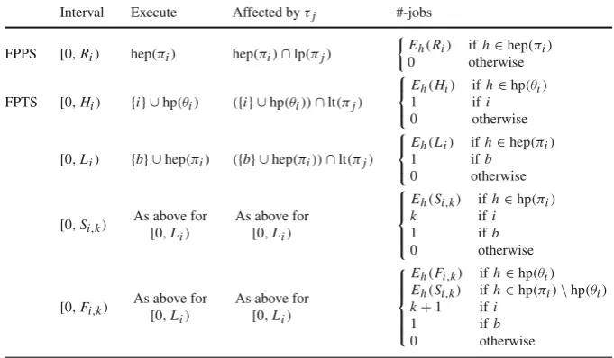
An overview of these tasks for the response interval[0,Ri)is given in Table2, i.e. the table shows
Table 2 Overview of tasks that can execute and affect the execution of taskτi in a level-iactive period
starting at timet=0 for both FPPS with constrained deadlines and FPTS with arbitrary deadlines, assuming a taskτbthat blocksτifor FPTS, i.e.b∈b(i)
Interval Execute Affected byτj #-jobs
FPPS [0,Ri) hep(πi) hep(πi)∩lp(πj)
Eh(Ri) ifh∈hep(πi)
0 otherwise
FPTS [0,Hi) {i} ∪hp(θi) ({i} ∪hp(θi))∩lt(πj)
⎧ ⎨ ⎩
Eh(Hi) ifh∈hp(θi)
1 ifi
0 otherwise
[0,Li) {b} ∪hep(πi) ({b} ∪hep(πi))∩lt(πj)
⎧ ⎨ ⎩
Eh(Li) ifh∈hep(πi)
1 ifb
0 otherwise
[0,Si,k)
As above for [0,Li)
As above for [0,Li)
⎧ ⎪ ⎪ ⎨ ⎪ ⎪ ⎩
Eh(Si,k) ifh∈hp(πi) k ifi
1 ifb
0 otherwise
[0,Fi,k) As above for[0,L i)
As above for [0,Li)
⎧ ⎪ ⎪ ⎪ ⎨ ⎪ ⎪ ⎪ ⎩
Eh(Fi,k) ifh∈hp(θi) Eh(Si,k) ifh∈hp(πi)\hp(θi) k+1 ifi
1 ifb
0 otherwise
• Execute:The tasks that can execute jobs in the interval, being tasks with a priority higher than or equal to the priority ofτi, i.e. hep(πi);
• Affected byτj: The set of tasks that (i) can execute jobs in the intervaland(ii) can be pre-empted by taskτj, i.e. hep(πi)∩lp(πj);
• #-jobs:The number of job activations of a task that canexecutein the interval, i.e. Eh(Ri)for each taskτh∈hep(πi).
The “ #-jobs” in the interval[0,Ri)can be immediately derived fromRi, see (8). If
Ri ≤ Di ≤ Ti, thenEi(Ri)=1 and, as a result, taskτi can be treated as any other task.
When we focus only on the pre-empting tasks, e.g. when using the ECB-Only approach, we only need the information of the rowaffected byτj in Table2; see (10). When we consider the pre-empted tasks, e.g. when using the UCB-Only Multiset approach, the #-jobsalso play a role. To be more specific, the multisetMiucb-o,j (t)in (12) contains Ej(Rh)copies of the size of UCBh for each of theEh(t)jobs of task
τh, withh∈aff(πi, πj), affectingτi and affected byτj.
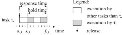
Fig. 2 The response time and hold time of jobkof taskτi
taskτi
time ai,k fi,k
response time
execution by other tasks than τi
execution by τi
release Legend:
si,k hold time
5.2 Bounding the number of pre-emptions using hold times
For FPPS with constrained deadlines, all pre-emptions during the response time of a job of a task may actually evict UCBs of that job. For FPTS, however, some pre-emptions can only take place between the activation and the start of a job, and therefore do not evict UCBs of that job. An obvious example is a non-pre-emptive task, where no pre-emption can take place during the actual execution of its jobs.
To prevent pessimism in the analysis when focussing on pre-empted tasks, we consider so-called hold times. To that end, we distinguish the (absolute)activation time ai,k, (absolute)start-time si,kand (absolute)finishing time fi,kof a jobkof task
τi; see Fig.2. The lengths of the intervals[ai,k, fi,k)and[si,k,fi,k)are termed the
response time Ri,kand thehold time4 Hi,k of jobkof taskτi, respectively.
Under FPPS, the worst-case hold timeHiof a taskτican be calculated by means of (8), i.e. by using the equation to determine the worst-case response timeRi for FPPS with constrained deadlines; see Bril (2004) andBril et al.(2008). Under FPTS, only tasks with a priority higher than the pre-emption thresholdθi can pre-empt taskτi. Hence, the worst-case hold timeHi (without CRPD) is given by
Hi =Ci+
∀j∈hp(θi)
Ej(Hi)·Cj. (18)
We will now show that the worst-case hold time is both a proper value to determine an upper bound for the number of pre-emptions of a job of taskτi as well as a potential improvement over using the worst-case response time Ri. This allows us to tighten the number of pre-emptionsEj(Rh)byEj(Hh)in the construction of the multisets for the approaches consideringpre-empted tasks.
Being theworst-casehold timeHi of a taskτi,Hi is an upper bound for the hold time for every job ofτiin general and for every job in the level-iactive period with a worst-case lengthLiin particular. The former is an immediate consequence of the fact that the tasks that can influence the hold time of an individual jobkofτi are identical to those that can influence Hi, i.e. hp(θi). The latter follows from the observation that a critical instant to determine the worst-case response timeRi is not necessarily a critical instant for the worst-case hold timeHi, hence∀0≤k<Ei(Li)Hi,k ≤ Hi. The
4 The notion ofhold timeis inspired by the termresource hold timesin Bertogna et al. (2007) and the
[image:17.439.174.388.62.123.2]worst-case hold time Hi is therefore a proper value to determine an upper bound on the number of pre-emptions of a job of taskτi.
The worst-case hold timeHiof a taskτiis at most equal to the worst-case response timeRi ofτi, i.e.Hi ≤Ri. This result immediately follows from the fact that the set of tasks that influences the worst-case hold timeHi of taskτi is a subset of the set of tasks that influences the worst-case response time Riofτi. The worst-case hold time
Hiof a taskτimay be smaller than the worst-case response time Ri. This is because (i) the potential delay of the execution of a job by a previous job (Bril et al. 2008), (ii) the blocking by a taskτbwithb ∈b(i), and (iii) the interference of tasksτj with
j∈hp(πi)∩lep(θi)are included inRi but not inHi. Example2below illustrates (i) and Example3illustrates (ii) and (iii).
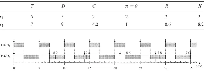
Example 2 The characteristics of a setT2of periodic tasks is given in Table3. The
timeline shown in Fig.3illustrates both the worst-case hold timeH2 =8.2 and the
worst-case response timeR2=8.6 for the job activated at timet =14. R2is larger
thanH2, because R2includes a delay of 0.4 of the job activated at timet =7. This
illustrates (i).
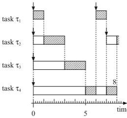
Example 3 The characteristics of a setT3of periodic tasks are given in Table4. The
[image:18.439.52.390.362.481.2]worst-case hold times of all tasks aresmallerthan their worst-case response times. Taskτ1is an example of (ii), taskτ4is an example of (iii), and tasksτ2andτ3are examples of both (ii) and (iii).
Table 3 Task characteristics ofT2and worst-case response times and hold times of periodic tasks with
non-constrained deadlines under FPPS without CRPD
T D C π=θ R H
τ1 5 5 2 2 2 2
τ2 7 9 4.2 1 8.6 8.2
30 20
10
0 5 15 25 35
taskτ1
taskτ2
time 0 . 7 8
. 7 6
. 8 4
. 7 2
. 8
Fig. 3 Timeline forT2for an entire hyper period (i.e. lcm(T1,T2)=35) with a simultaneous release of
τ1andτ2at timet=0. Thenumbers to the top right corner of the boxesdenote the response times of the
[image:18.439.169.388.528.601.2]respective job activations
Table 4 Task characteristics of T2and worst-case response
times and hold times of periodic tasks under FPTS without CRPD
T=D C π θ R H
τ1 6 1 4 4 3 1
τ2 7 2 3 4 5 2
τ3 9 2 2 3 8 3
Fig. 4 Taskτ1is activated
twice during the worst-case response time of taskτ4but only
once during the worst-case hold time ofτ4
0 5
taskτ3
taskτ4
time 8 taskτ1
taskτ2
Tasksτ3andτ4of Example3are particularly interesting when FPTS is extended
with CRPD, because taskτ1can be activated twice during their worst-case response
time but only once during their worst-case hold time; see Fig.4.
5.3 Determining the tasks that can execute and are affected byτj
Having introduced the worst-case hold timeHiof taskτi, we now determine for each of the intervals[0,Hi),[0,Li),[0,Si,k), and[0,Fi,k)the tasks that can execute in the interval (“execute”) and from these tasks those that are affected by taskτj(“affected
byτi”) for FPTS in Table2.
The tasks that can execute in[0,Hi)can immediately be derived from (18), i.e. taskτiand all tasks with a priority higher than the pre-emption thresholdθiof taskτi. This set of tasks is therefore characterized by the set of indices{i} ∪hp(θi). Similarly, the set of tasks that can execute in[0,Li),[0,Si,k), and[0,Fi,k)can immediately be derived from (3), (5), and (6), respectively. Assuming a taskτb that blocksτi, i.e.
b∈b(i), all these three sets are characterized by the set of indices{b} ∪hep(πi). To determine the “affected byτj” for each of these intervals, we simply take the intersection of the set of indices for “execute” with lt(πj), similar to FPPS.
5.4 Determining the number of job activations “ #-jobs”
We now show that we can derive the “ #-jobs” for FPTS in Table2from the equations corresponding to the intervals, similar to FPPS. We start with the interval[0,Hi). The intervals[0,Li),[0,Si,k)and[0,Fi,k)are subsequently addressed for Bi = 0 and
Bi =0.
5.4.1#-jobs for[0,Hi)
[image:19.439.255.385.57.177.2]Example 4 We reconsiderT2 of Example2. For that example, E2(H2) = 2 rather
than 1. To prevent this pessimism, we take exactly one activation ofτiinto account.
5.4.2#-jobs for[0,Li),[0,Si,k), and[0,Fi,k)when Bi =0
Given a taskτb that blocksτi under FPTS, i.e.b ∈ b(i), the number of activations #-jobsin the intervals[0,Li),[0,Si,k)and[0,Fi,k)in Table2 can be immediately derived from (3) for Li, (5) forSi,k and (6) forFi,k. To prevent pessimism, exactly one activation ofτbis taken into account. Similarly, exactlykandk+1 jobs ofτi are taken into account when determiningSi,kandFi,k, respectively.
Example 5 We reconsiderT2of Example2. The worst-case finalization timeF2,0of the first job ofτ2is equal to 8.2. Because E2(8.2) =2, (12) would include 2 jobs
ofτ2inM2,1ucb-o(8.2)rather than 1. To prevent this pessimism, we explicitly take the
number of jobs ofτi into account.
5.4.3#-jobs for[0,Li),[0,Si,k), and[0,Fi,k)when Bi =0
Lemma1shows thatE∗j(Si,k)can be replaced byEj(Si,k)for the caseBi =0 in (6) forFi,k.
Lemma 1 Let j ∈hp(πi)and assume a level-i active period starting at time t =0
with a simultaneous release ofτi andτj. Let Si,k denote the worst-case start time
of job k ofτi in that level-i active period and be derived by (5). Now the following
equality holds:
∀j∈hp(πi)E
∗
j(Si,k)=Ej(Si,k). (19)
Proof The termE∗j(Si,k)represents the maximum number of activations ofτj in the interval[0,Si,k]. When∃m∈NSi,k =m·Tj, taskτjis activated at timeSi,k. This would imply thatτi cannot start atSi,k, which contradicts the definition ofSi,k. We therefore conclude that∄m∈NSi,k=m·Tj. As a result,E∗j(Si,k)=Ej(Si,k), which proves the
lemma. ⊓⊔
Corollary 1 We may simplify(6)by replacing E∗j(Si,k)by Ej(Si,k)and ignoring the
case distinction, i.e.
Fi,k =Si,k+Ci +
∀j∈hp(θi)
Ej(Fi,k)−Ej(Si,k)
·Cj. (20)
Similarly, Lemma2shows thatγi,j(t)can be defined in terms of Ej(Si,k)rather thanE∗j(Si,k)for the caseBi =0 in (5) when determiningSi,k.
Lemma 2 When Si,k is extended with a termγi,k(t)for the case Bi =0, γi,k(t)can
Proof A solution for the recurrent relation forSi,k is found whenSi(ℓ),k = Si(ℓ,k+1) for two subsequent iterations. ForSi(ℓ),k there are two cases, eitherEj(Si(ℓ),k)=E∗j(Si(ℓ),k)or
Ej(Si(ℓ),k)= E∗j(Si(ℓ),k).
Let Ej(Si(ℓ),k)= E∗j(Si(ℓ),k), i.e.∄m∈NSi(ℓ),k =m·Tj. As a result, it doesn’t matter whetherEj(t)orE∗j(t)is used inγi,k(t).
Now let Ej(Si(ℓ),k)= E∗j(Si(ℓ),k), i.e.∃m∈NSi(ℓ),k =m·Tj. As a result, an additional activation ofτj will be taken into account when determiningSi(ℓ,k+1), irrespective of using eitherEj(t)orE∗j(t)inγi,k(t). Together, these two cases prove the lemma. ⊓⊔
We therefore conclude that, apart from the number of job activations of τb, the information in Table2also holds forτi whenBi =0.
5.5 Identifying the task causing the largest blocking delay
A nice property of FPTS is that just one job of lower priority is able to cause blocking delays. In the presence of CRPD, however, the largest computation time among the blocking tasks does not necessarily result in the largest worst-case response time.
Example 6 We reconsiderT3of Example3. Without CRPD, the blocking ofτ2due
toτ3andτ4is the same becauseC3=C4, i.e.B2=max(0,max{C3,C4})=1. The
blocking including CRPD may be different, however, due to different UCBs ofτ3and
τ4and the ECBs ofτ1. Even asmallercomputation time of a blocking task may result
in alargeroverall blocking effect when CRPD is included.
For the case with blocking (Bi =0), we therefore need a more complex procedure to compute response times. Our new procedure determines the values forLi,Si,k,Fi,k, andRi with CRPD by taking the maximum value over all tasks that may blockτi.
5.6 Termination of the iterative procedure forLi
Termination of the iterative procedure to determineLi is no longer guaranteed when
U <1, because the CRPD is not taken into account in the utilizationU. To address this problem, we first observe that by definition every level-iactive period, with 1≤i<n, is contained in a level-n active period (Bril et al. 2009). Hence, termination of the iterative procedure to determineLnguarantees termination forLi for all 1≤i <n. Next, the lowest priority taskτncannot be blocked. As a result, whenLnexceeds the least common multiple (LCM) of the periods of the task setT, the iterative procedure
5.7 Applying the results
In this section, we studied various preliminaries for the integration of CRPD in the analysis for FPTS. In the following sections, we apply the achieved results. In partic-ular, we
• apply the notion of worst-case hold time by using Ej(Hh)rather than Ej(Rh) to tighten the number of times thatτj may pre-empt a job of τh for approaches consideringpre-emptedtasks. This influences the definition of the multisetMi,j for the UCB-Only Multiset approach, the ECB-Union Multiset approach, and the UCB-Union Multiset approach.
• apply the derived “affected byτj” information in the definitions ofγi,j andMi,j for the various approaches. This requires an extension of the subscripts ofSi,k,
Fi,k, γi,j andMi,jwithbfor those cases where a taskτbmay block a taskτi.
• apply the derived “#-jobs” information for approaches considering pre-empted tasks. This requires a case distinction following the information in Table2in the definition of the multiset Mi,j. Moreover, it requires a further extension of the subscripts ofγi,jandMi,jwithk, and the introduction of an additional parameter for bothγi,j andMi,j to cater for the pre-emptions in the intervals corresponding to the worst-case start-time and the worst-case finalization time.
• take the maximum value over all tasks that may blockτito determineLiandFi,k, whenτi can be blocked.
6 FPTS with CRPD: pre-empting tasks
In this section, we consider the ECB-Only approach, i.e. focus only on thepre-empting tasks. Because the worst-case hold timeHiand the row #-jobsin Table2only play a role for pre-empted tasks, we ignoreHi and #-jobsin this section. In order to extend the equations forLi,Si,kandFi,kfor FPTS with a termγi,j(t), we must adaptγiecb-o,j (t) by considering the tasks affected by taskτj (see the rowaffected byτj in Table2). As shown in Table2, the tasks being affected by pre-emptions are the same for the intervals[0,Li),[0,Si,k), and[0,Fi,k), but differ from the tasks being affected under FPPS with constrained deadlines. We therefore generalize, i.e. redefine, the set of tasks aff(πi, πj)for FPTS to
aff(πi, πj)def= hep(πi)∩lt(πj). (21)
Because a task may but need not be blocked, we excluded “{b}” from (21) and will use dedicated clauses to treat blocking tasks in the sequel. Equation (21) for FPTS specializes to (11) for FPPS because lp(πj)=lt(πj)for FPPS.
6.1 Worst-case lengthLi
For a taskτiwithout blocking (Bi =0), we can find an upper bound forLiwith CRPD by extending (3) withγi,j(t), similar to the extension ofRiin (9), i.e.
Li =
∀j∈hep(πi)
Ej(Li)·Cj+γi,j(Li)
. (22)
For the ECB-Only approach, we can subsequently reuse (10) forγi,j(t)with aff(πi, πj) as defined in (21).
For the case Bi =0, we rewrite (3) forLi by distributing addition over the inner-max operation in equation (4) for Bi and subsequently extending the equation for CRPD as explained in Sect.5.5, i.e.
Li = max ∀b∈b(i)
⎛ ⎝Cb+
∀j∈hep(πi)
Ej(Li)·Cj +γi,j,b(Li) ⎞
⎠. (23)
A subscript “b” has been introduced inγi,j,b(t)to capture the CRPD related to the blocking taskτb. For the ECB-Only approach,γi,j,b(t)is defined as
γiecb-o,j,b (t)=
BRT·Ej(t)· ECBj
if aff(πi, πj)= ∅ ∨b∈lt(πj)
0 otherwise . (24)
Compared to (10) for FPPS, the first clause forγiecb-o,j,b (t)in (24) for FPTS has been extended withb∈lt(πj), becauseτjmay in that case also pre-empt taskτb. Note that
({b} ∪hep(πi))∩lt(πj)in Table2is equal to aff(πi, πj)∪({b} ∩lt(πj))in (24).
6.2 Worst-case start timeSi,k
Similar toLi, we extend Eq. (5) forSi,kwith a termγi,k(t)to include CRPD for tasks without blocking, i.e.
Si,k =kCi +
∀j∈hp(πi)
E∗j(Si,k)·Cj+γi,j(Si,k)
. (25)
Based on Lemma2, we conclude that we can defineγi,j(t)in terms of Ej(t)rather thanE∗j(t). Hence, we can also reuseγiecb-o,j (t)from (10) for the ECB-Only approach, i.e. we use aff(πi, πj)as defined in (21), similar toLi.
For tasks with blocking, we extendSi,kwith an additional subscript “b” and a term
Si,k,b=Cb+kCi+
∀j∈hp(πi)
Ej(Si,k,b)·Cj +γi,j,b(Si,k,b)
. (26)
For the ECB-Only approach, we can reuseγiecb-o,j,b (t)from (24) forγi,j,b(t), similar to
Li.
6.3 Worst-case finalization timeFi,k
For tasks without blocking, we can extend (20) with γi,j(t)terms complementing
Ej(Fi,k)·Cj andEj(Si,k)·Cj, i.e.
Fi,k =Si,k+Ci+
∀j∈hp(θi)
Ej(Fi,k)−Ej(Si,k)
·Cj
+
∀j∈hp(θi)
γi,j(Fi,k)−γi,j(Si,k)
. (27)
Similar toLi andSi,kwe use (10) forγi,k(t), with aff(πi, πj)as defined in (21). Similar toSi,k, we add a subscript “b” to Fi,k for tasks with blocking. Similar to the caseBi =0, we expand the formula with terms for CRPD, i.e.
Fi,k,b=Si,k,b+Ci+
∀j∈hp(θi)
Ej(Fi,k,b)−Ej(Si,k,b)
·Cj
+
∀j∈hp(θi)
γi,j,b(Fi,k,b)−γi,j,b(Si,k,b)
. (28)
The subtracted termγi,j,b(Si,k,b)in (28) prevents the cache-related pre-emption costs already covered in (26) forSi,k,bbeing accounted for twice. Similar toLiandSi,k, we apply (24) forγi,j,b(t). To compute Fi,k, we take the maximum value over all tasks that may blockτi, similar toLi and as explained in Sect.5.5, i.e.
Fi,k= max
∀b∈b(i)Fi,k,b. (29)
7 FPTS with CRPD: pre-empted tasks
7.1 Worst-case hold timeHi
We can find an upper bound forHiwith CRPD by extending (18) withγi,j(t), similar to the extension ofRi withγi,j(t), i.e.
Hi =Ci+
j∈hp(θi)
Ej(Hi)·Cj+γi,j(Hi)
. (30)
Although we can applyγiucb-o,j (t)in (13) forγi,j(t)in (30) for the UCB-Only Multiset approach, we need to adapt the definition of Miucb-o,j (t)in (12) to prevent pessimism and use the proper set of affected tasks, as discussed in Sects.5.2,5.3and5.4. Firstly, worst-case hold times are to be considered for pre-empted tasks, rather than worst-case response times. Secondly, the set of affected tasks is to be adapted to({i} ∪hp(θi))∩ lt(πi); see Table2. Finally, exactly one job of taskτi needs to be considered rather thanEi(t)jobs, requiring a dedicated clause. These three adaptations of (12) result in
Miucb-o,j (t)=
h∈hp(θi)∩lt(πj) ⎛ ⎝
Ej(Hh)·Eh(t) UCBh ⎞ ⎠∪ ⎧ ⎪ ⎨ ⎪ ⎩
Ej(Hi) UCBi
ifi∈lt(πj)
∅ otherwise
.
(31)
7.2 Worst-case lengthLi
Similar to the ECB-Only approach, we can use (23) to find an upper bound forLi by extending (13) forγiucb-o,j (t)with a subscriptbfor the blocking taskτb, withb∈b(i):
γiucb-o,j,b (t)= BRT ·
Ej(t)
ℓ=1
sort
Miucb-o,j,b(t)
[ℓ]. (32)
The definition of Miucb-o,j (t)in (12) also needs to be extended with a subscriptb, to consider exactly one blocking job ofτbrather thanEb(t)jobs; see Table2.
Miucb-o,j,b(t)=
h∈aff(πi,πj) ⎛ ⎝
Ej(Hh)·Eh(t) UCBh ⎞ ⎠∪ ⎧ ⎪ ⎨ ⎪ ⎩
Ej(Hb) UCBb
ifb∈lt(πj)
∅ otherwise
.
7.3 Worst-case start timeSi,k
As well as considering exactly one job of task τb, the definitions ofγiucb-o,j,b (t)and
Miucb-o,j,b(t)are further extended forSi,k to consider exactlykjobs ofτi (see Table2), i.e.
γiucb-o,j,k,b(t)= BRT ·
Ej(t)
ℓ=1
sort
Miucb-o,j,k,b(t)[ℓ] (34)
and
Miucb-o,j,k,b(t)=
h∈aff(πi,πj)\{i} ⎛ ⎝
Ej(Hh)·Eh(t) UCBh ⎞ ⎠∪ ⎧ ⎪ ⎨ ⎪ ⎩
Ej(Hi)·k UCBi
ifi∈lt(πj)
∅ otherwise ∪ ⎧ ⎪ ⎨ ⎪ ⎩
Ej(Hb) UCBb
ifb∈lt(πj)
∅ otherwise
. (35)
Similar toHi, taskτi is again treated by a separate clause, which makes it necessary to use aff(πi, πj)\ {i}rather than aff(πi, πj). Moreover, Miucb-o,j,k,b(t)is based on the worst-case hold times of the tasksτh, τi, andτbrather than their worst-case response times.
Similar to the ECB-Only approach, a subscript “b” is added toSi,k, and the equation ofSi,kin (5) is extended withγi,j,k,b(t)as follows:
Si,k,b=Cb+kCi +
∀j∈hp(πi)
Ej(Si,k,b)·Cj+γi,j,k,b(Si,k,b)
. (36)
7.4 Worst-case finishing time Fi,k
As indicated in Table 2, exactlyk +1 jobs ofτi need to be considered for Fi,k. Moreover, we need to split the set of tasks hp(πi)into two subsets forFi,k, i.e. the set hp(πi)\hp(θi)of tasks that can be blocked byτi and the set hp(θi)that cannot be blocked byτi. The former set can execute and experience pre-emptions in[0,Si,k), whereas the latter set can execute and experience pre-emptions in[0,Fi,k). To take the proper number of activations of tasks in these two sets into account, we use two parameterstsandtf forγiucb-o,j,k,bandMiucb-o,j,k,b, i.e.
γiucb-o,j,k,b(ts,tf)= BRT · Ej(tf)
ℓ=1
sort
Miucb-o,j,k,b(ts,tf)
and
Miucb-o,j,k,b(ts,tf)=
h∈((aff(πi,πj)\{i})∩hp(θi))
Ej(Hh)·Eh(tf)
UCBh ∪
h∈((aff(πi,πj)\{i})\hp(θi))
Ej(Hh)·Eh(ts)
UCBh ∪ ⎧ ⎪ ⎨ ⎪ ⎩
Ej(Hi)·(k+1)
UCBi
ifi∈ lt(πj)
∅ otherwise ∪ ⎧ ⎪ ⎨ ⎪ ⎩
Ej(Hb)
UCBb
ifb∈ lt(πj)
∅ otherwise
. (38)
Similar to the ECB-Only approach,Fi,kis extended with a subscript “b” andγi,j,k,b terms, i.e.
Fi,k,b=Si,k,b+Ci
+
∀j∈hp(θi)
Ej(Fi,k,b)−Ej(Si,k,b)
·Cj
+
∀j∈hp(θi)
γi,j,k,b(Si,k,b,Fi,k,b)−γi,j,k,b(Si,k,b)
. (39)
The termγi,j,k,b(Si,k,b)in (39) prevents the cache-related pre-emption costs already covered in (36) forSi,k,bbeing accounted for twice.
We may subsequently determine Fi,k by (29) and can derive Ri through (7) as before.
8 FPTS with CRPD: pre-empting and pre-empted tasks
In this section, we consider the ECB-Union and UCB-Union Multiset approaches, i.e. we consider both the pre-empting and the pre-empted tasks. As described in Sect. 4.2for FPPS with CRPD, the definitions of the multisets for the ECB-Union and UCB-Union Multiset approaches can be derived from the definition of the multi-set for the UCB-Only Multimulti-set approach. A similar derivation applies for FPTS with CRPD. We therefore only consider the definition of the multisetsMiecb-u,j,k,b(ts,tf)and
Miucb-u,j,k,b(ts,tf)for the worst-case finalization timeFi,kfor the case with blocking. The derivation of the definitions for the case without blocking and for the worst-case hold timeHi, worst-case lengthLi and worst-case start timeSi,kare similar.
8.1 ECB-Union Multiset approach