This is a repository copy of
Renewable energy sharing among base stations as a
min-cost-max-flow optimization problem
.
White Rose Research Online URL for this paper:
http://eprints.whiterose.ac.uk/139707/
Version: Accepted Version
Article:
Benda, D., Chu, X. orcid.org/0000-0003-1863-6149, Sun, S. et al. (2 more authors) (2018)
Renewable energy sharing among base stations as a min-cost-max-flow optimization
problem. IEEE Transactions on Green Communications and Networking. ISSN 2473-2400
https://doi.org/10.1109/TGCN.2018.2876005
© 2018 IEEE. Personal use of this material is permitted. Permission from IEEE must be
obtained for all other users, including reprinting/ republishing this material for advertising or
promotional purposes, creating new collective works for resale or redistribution to servers
or lists, or reuse of any copyrighted components of this work in other works. Reproduced
in accordance with the publisher's self-archiving policy.
[email protected] https://eprints.whiterose.ac.uk/ Reuse
Items deposited in White Rose Research Online are protected by copyright, with all rights reserved unless indicated otherwise. They may be downloaded and/or printed for private study, or other acts as permitted by national copyright laws. The publisher or other rights holders may allow further reproduction and re-use of the full text version. This is indicated by the licence information on the White Rose Research Online record for the item.
Takedown
If you consider content in White Rose Research Online to be in breach of UK law, please notify us by
Renewable Energy Sharing among Base Stations
as a Min-Cost-Max-Flow Optimization Problem
Doris Benda,
Student Member, IEEE,
Xiaoli Chu,
Senior Member, IEEE,
Sumei Sun,
Fellow, IEEE,
Tony Q.S. Quek,
Fellow, IEEE,
and Alastair Buckley
Abstract—Limited work has been done to optimize the power sharing among base stations (BSs) while considering the topology of the cellular network and the distance-dependent power loss (DDPL) in the transmission lines. In this paper, we propose two power sharing optimization algorithms for energy-harvesting BSs: the max-flow (MF) algorithm and the min-cost-max-flow (MCMF) algorithm. The two proposed algorithms minimize the power drawn from the main grid by letting BSs with power surpluses transmit harvested power to BSs with deficits. The MCMF algorithm has an additional DDPL cost associated with each transmission line. Hence, the MCMF algorithm shares the harvested power over shorter distances and loses less power during the transmission than the MF algorithm. Our numerical results show that for a fully connected cellular network, i.e., every pair of BSs can share power, with a moderate power loss coefficient perl (∈R+)meters of transmission line, the MCMF
algorithm saves up to 10%, 22%, and 30% more main grid power than the MF algorithm for 5, 10, and15 BSs uniformly distributed in a square area of l2 square meters, respectively.
Index Terms—Cellular network, min-cost-max-flow, max-flow, energy harvesting, energy sharing
I. INTRODUCTION
More than half of the energy consumption in the cellular network infrastructure is caused by the operation of base stations (BSs) [2]. In addition, environmental policies promote the incorporation of environmentally friendly technologies. As a result, BSs equipped with energy-harvesting devices, e.g. solar cells, are becoming increasingly attractive to cellular network operators [3], [4]. Furthermore, cellular networks capable of energy-harvesting are more sustainable and resilient during natural disasters than conventional grid-connected ones [2].
Manuscript received ######; revised ######. This work was partially presented at VTC-Spring 2018 [1]. This work is supported by the A*STAR Industrial Internet of Things Research Program, under the RIE2020 IAF-PP Grant A1788a0023, and the A*STAR Research Attachment Program. This work is partly funded by the European Unions Horizon 2020 Research and Innovation Programme under grant agreement No 645705.
D. Benda, and X. Chu are with the department of Electronic and Elec-trical Engineering, University of Sheffield, The United Kingdom, e-mail: [email protected], and [email protected].
D. Benda and S. Sun are with the Communications and Networks Cluster, Institute for Infocomm Research, Singapore, e-mail: [email protected] and [email protected].
T. Q.S. Quek is with the Information Systems Technology and Design Pillar, Singapore University of Technology and Design, Singapore, e-mail: [email protected].
A. Buckley is with the department of Physics and Astronomy, University of Sheffield, The United Kingdom, e-mail: [email protected].
A. Different Power Sharing Methods
The amount of harvested power as well as the power consumption of the BSs vary over time and space resulting in power surpluses or power deficits at the BSs. To avoid wasting precious harvested power, power can be transmitted from surplus BSs to deficit BSs via transmission lines. Other options for power sharing are wireless power transfer, traffic offloading to neighboring BSs, smart grid/ main grid trading and batteries. In the following, we will discuss these options separately and compare them with power sharing via direct transmission lines.
1) Wireless Power Transfer: Power can be shared through
wireless power transfer. Nonetheless, this is limited to very short distances due to the high power losses associated with long wireless power transmission [5].
2) Traffic Offloading To Neighboring BSs: The authors in
[6] propose to offload user equipments (UEs) at the cell edge of BSs with power deficit to neighboring BSs with abundant renewable energy. Nonetheless, this causes a deterioration in the signal-to-interference-plus-noise ratio (SINR) of the offloaded UEs, whereas power sharing via direct transmission lines does not affect the SINR.
3) Smart Grid/ Main Grid Trading: The authors in [7], [8]
propose to sell and buy power from the grid and use the grid to conduct virtual power transfer in addition to power sharing via direct transmission lines. Power sharing via direct transmission lines requires high capital expenditure for deploying physical transmission lines whereas grid trading implies operational expenditure in the form of a price that has to paid to the grid operator. To evaluate if the initial investment for deploying physical transmission lines is justified in the long-term or each BS should rather sell and buy its power from the grid, the local price structure has to be evaluated. BSs can buy power from the grid at a price pb and sell it to the grid at a price ps, where the grid operator typically requires that pb > ps. The
difference in price denoted by∆pis as follows:∆p=pb−ps.
If∆pis great, it is more cost efficient to share power via direct
transmission lines. If ∆p is small, it is more cost efficient to
sell and buy power from the grid. Even if∆pis small, cellular
transformers are not needed, and DC to AC conversion losses are negligible if DC transmission lines are deployed between DC energy harvesters such as solar cells. In contrast, sparse cellular networks with long inter-site distances are not suitable for power sharing via direct transmission lines due to the high power loss during transmissions, the high capital expenditure, and the right-of-way clearance needed for the transmission corridors. In the latter case, power will be more likely bought and sold to the grid.
4) Batteries: Since batteries are expensive and have a short
lifetime (3-9 years), battery replacements significantly con-tribute to the system lifetime cost [9]. Employing both, direct transmission lines for power sharing and batteries to balance the mismatch between the power generation and consumption at the BSs would greatly increase the capital expenditure. Hence, we only use direct transmission lines in our system model to reduce the capital expenditure.
B. Justification For Power Surpluses And Deficits At Neigh-boring BSs
It has been shown that 80% of grid power can be saved if power sharing is enabled between two energy-harvesting BSs with anti-correlated energy profiles [10]. Meanwhile, considering the power loss along the transmission lines, it is preferred to share power among BSs that are not far away from each other. Anti-correlated energy generation profiles at neighboring BSs can be obtained by different types of energy harvesters.
For example, a solar cell and a wind turbine in the same area can achieve anti-correlated energy generation profiles on a daily timescale due to the fact that high (low) pressure areas tend to be sunny (cloudy) with low (high) surface wind, and on a seasonal timescale due to the fact that more solar (wind) energy can be harvested in summer (winter) than in winter (summer) [3]. If only solar cells are available for deployment, anti-correlated energy profiles at neighboring BSs can be achieved by deploying southeast orientated solar cells and southwest orientated solar cells, respectively (cf. Fig. 3 in [4]), where a southeast (southwest) orientated solar cell has an orientation angle of−45°(45°)with respect to the southern direction [4].
Furthermore, even if two BSs have similar energy gener-ation profiles, different traffic loads at the BSs may result in power surpluses and deficits as well, because the power consumption profiles at the BSs are traffic load-dependent and can be different (cf. [11]).
C. Background Of The Used Optimization Algorithms
We propose two power sharing optimization algorithms based on the max-flow (MF) problem and the min-cost-max-flow (MCMF) problem, which are well known for their low computational complexity. For a flow network with|E|edges and |V| vertices, the MF problem and the MCMF problem can be efficiently solved inO(|V|2|E|)(general push-relabel algorithm [12]) andO(|E|log|E|(|E|+|V|log|V|))(Orlin’s algorithm [13]), respectively. In practice, network simplex
algorithms are commonly used to solve the MF problem and the MCMF problem as well [13].
D. Current Knowledge Gaps
There are three main issues that have not been sufficiently studied in the current literature:
1) Distance-dependent Power Loss In Transmission Lines: Transmitting power over longer distances will result in higher resistive power losses, but most existing works do not include distance-dependent power loss (DDPL) in their system model. For example, [14] introduced an energy hub for power sharing in cellular networks and assumed that the resistive power loss in the transmission lines is independent of the power propagation distance.
2) Topology Of The Cellular Network: Most existing works
consider sharing power among only a few BSs, e.g., two BSs in [10] and three BSs in [8], without systematically considering the topology of the cellular network. In this paper, we generalize the BS power sharing scenario to a dense cellular network, where the topology of the cellular network is incorporated in the system model and the harvested renewable power is shared among nearby BSs.
3) Performance Gain vs. Complexity Of Power Loss Aware
Power Sharing Algorithms: To the best of our knowledge,
this work is the first to investigate the trade-off between the performance gain and the computational complexity of BS power sharing algorithms with or without considering the transmission line power loss. Moreover, the main difference to [7] is that we evaluate the performance gains that a power loss aware power sharing algorithm can achieve in different cellular networks and derive guidelines on power loss aware power sharing for different cellular network deployment scenarios.
E. Contributions
The main contributions of this paper address the identified knowledge gaps as follows:
• We propose a BS power sharing model for
energy-harvesting enabled dense cellular networks and incorpo-rate into the BS power sharing model the topology of the cellular network and the DDPL in the transmission lines.
• We develop an MF algorithm and an MCMF algorithm
which both minimize the power drawn from the main grid by letting BSs with surpluses transmit harvested power to BSs with deficits. The MCMF algorithm has an additional DDPL cost associated with each transmission line and therefore reduces the power losses during the transmission.
• We derive a closed-form expression of the average total power drawn from the main grid by all the BSs for the MF algorithm on a complete neighboring graph. The accuracy of the closed-form expression is verified by the simulation results.
• We investigate the performance gap between the two
Based on the insights obtained, we provide guidelines on which of the two algorithms should be used under different scenarios of energy-harvesting enabled cellular networks.
The rest of this paper is organized as follows. Section II presents the system model. Section III formulates the MF/MCMF problem. Section IV proposes a linear optimiza-tion program to solve the MF/MCMF problem. Secoptimiza-tion V derives a closed-form expression of the average total power drawn from the main grid by the BSs for the MF algorithm. Section VI presents the performance evaluation results for both algorithms. Finally, the paper is concluded in Section VII.
II. SYSTEMMODEL
We considerN ∈Nuniformly distributed BSs in a square area of l2 square meters (cf. Fig. 1), which are denoted as
BSi, i ∈ {1, ..., N}. Each BS is equipped with an energy-harvesting device, e.g., a solar cell, as well as a main grid connection but no battery.
We denote the power surplus/deficit of BSi as Bi[W] in watts. A surplus (deficit) in power at BSi is indicated by a positive (negative) value Bi. The objective is to balance out
the power in the network by transmitting power from surplus BSs to deficit BSs so that the total power drawn from the main grid by the deficit BSs is minimized. ABSiwithBi= 0will not take part in the power sharing scheme.
The set of surplus BSs is denoted as BS+, and the set of deficit BSs is denoted as BS−, i.e.,
BS+={i|Bi>0, i∈ {1, ..., N}},
BS−={i|Bi<0, i∈ {1, ..., N}}. (1)
For the network, the total power surplusB+, the total power deficit B−, and the net power surplus/deficit Bnet are given by
B+= X i∈BS+
Bi,
B−= X i∈BS−
Bi,
Bnet= N
X
i=1
Bi=B++B−.
(2)
BSs can be connected by a transmission line in a cellular network. As depicted in Fig. 2, the network is represented by a neighboring graph, where vertices denote BSs and edges denote transmission lines. Two BSs can share power between each other only if they are connected by an edge. BSs that are connected by an edge are referred to as neighboring BSs.
Sharing power between two BSs will result in some power loss as heat along the transmission line known as resistive heating. The power lossPloss[W]in watts in the transmission line can be calculated by Ohm’s law and the formula for the transmission line resistance [15] as follows:
Ploss=I2·ρ·
d Ac
, (3)
whereI[A]in amperes represents the current traveling through the transmission line, ρ[Ωm] in ohm-meters represents the resistivity of the transmission line,d[m]in meters represents the length of the transmission line, and Ac[m2] in square meters represents the cross-sectional area of the transmission line.
The power loss in the transmission line is proportional to its length as seen in (3). The power loss coefficientL(i, j)[Ω]
in ohms of the edge betweenBSi andBSj is defined as
L(i, j) = min(1,||BSi−BSj||
l ·C), (4)
where||BSi−BSj||[m] in meters is the Euclidean distance betweenBSiandBSj,l[m]in meters is the side length of the square in Fig. 2, andC[Ω]in ohms is the power loss coefficient per l meters of transmission line, which encapsulates the constants from (3) asC=Aρ·cl.L(i, j)is truncated to1because it is not possible to lose more than the available power.
[image:4.612.323.552.279.369.2]Fig. 1: Illustration of the considered cellular network, withN = 5BSs uniformly distributed in a square area ofl2square meters.
Fig. 2: The neighboring graph representation of the cellular network with example sur-plus/deficit power parametersBigiven for the
BSs.
III. THEMF/MCMF PROBLEM
We use the notation (i, j)to denote the edge between the surplusBSi and the deficitBSj, where(i, j)∈En indicates that BSi and BSj are connected by a transmission line, and the notationf[W] (i, j)
[W]andf[A2] (i, j)
[A2] for the power flow and the second power of the current flow on the edge from the surplus BSi to the deficitBSj, respectively.
A. Optimization Objective
Resistive heating is caused by the electric current of the power flow in the transmission line but not by the electric potential. Nonetheless, it is out of the scope of this paper to model the relationship between the power and the electric cur-rent in the transmission line. Thus, we assume for simplicity that the power flow in the transmission line is equivalent to the second power of the current flow in the transmission line. In other words, a power flow in the transmission line of x
watts, is equivalent to a current flow in the transmission line ofI=√xamperes in our system model. Hence,f[W] (i, j)
and f[A2] (i, j) have the same quantitative value for every
edge(i, j)but their units are different.
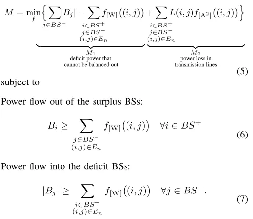
The optimization objective is to minimize the total power
M = min f
n X
j∈BS−
|Bj| −
X
i∈BS+ j∈BS−
(i,j)∈En
f[W] (i, j)
| {z }
M1
deficit power that cannot be balanced out
+X
i∈BS+ j∈BS−
(i,j)∈En
L(i, j)f[A2] (i, j)o
| {z }
M2
power loss in transmission lines
(5) subject to
Power flow out of the surplus BSs:
Bi ≥ X
j∈BS− (i,j)∈En
f[W] (i, j)
∀i∈BS+
(6)
Power flow into the deficit BSs:
|Bj| ≥ X
i∈BS+ (i,j)∈En
f[W] (i, j) ∀j∈BS−.
(7)
There are two scenarios in which a deficitBSi has to draw power from the main grid. On the one hand, a deficit BSi
may not have neighboring surplus BSs that have sufficient power to balance out the power deficitBi. On the other hand, even if the neighboring surplus BSs have sufficient power to balance out the power deficit Bi, due to the power losses in the transmission lines, the received power at the deficit BSi
is below the required deficit powerBi, so that the deficitBSi
has to offset this difference by drawing main grid power.
B. Definition Of The Flow Network
In the following subsections, we will show the conversion of the neighboring graph (cf. Fig. 2) and the optimization objective (cf. (5)-(7)) into a corresponding flow networkGand a corresponding MF/MCMF problem (cf. (14)-(17)), respec-tively. The optimization objective in form of an MF/MCMF problem can then be efficiently solved. The conversion steps in Figs. 3(a)-3(e) depict the conversion of Fig. 2 into a flow network as an example. The flow networkGis represented by the 4-tuple (V, E,s,t), where V, E,s, and t denote the set of vertices, the set of edges, the source vertex, and the sink vertex of the flow network, respectively. We use the notation
e = (i, j) to represent the directed edge e from vertex i to vertex j in the flow network.
1) Edges And Vertices (cf. Fig. 3(a)): Each surplus BS
is connected from the source vertex to the surplus BS by a directed edge. These edges are denoted as source edges Es. Each deficit BS is connected from the deficit BS to the sink vertex by a directed edge. These edges are denoted as sink edgesEt. If an edge exists between a surplus BS and a deficit BS in the neighboring graph, then the edge is replaced by a directed edge from the surplus BS to the deficit BS in the flow network. These edges are denoted as transmission edges
EBS. We do not allow power hopping in our system model
for simplicity1. The edges and vertices in the flow network are defined as follows:
Es={(s, j)|j ∈BS+},
Et={(i,t)|i∈BS−},
EBS={(i, j)|(i, j)∈En;i∈BS+;j∈BS−},
E =Es∪Et∪EBS∪(s,t),
V ={1,2, ..., N} ∪s∪t.
(8)
The power transmitted from BSi to BSj is modeled as
a flow along the path s −BSi − BSj − t in the flow network. To complete the conversion into a flow network, edge capacitiesu(e), edge costscM F(e)of the MF algorithm,
edge costscM CM F(e)of the MCMF algorithm and vertex
sup-plies/deficitsb(v)will be defined in the following subsections.
(a) Definition of edges and vertices
(b) Definition of the edge capacityu(e)
(c) Definition of the edge costcM F(e)
(d) Definition of the edge costcM CM F(e)
[image:5.612.48.305.70.293.2](e) Definition of the vertex supply/deficitb(v)
Fig. 3: Conversion of the neighboring graph in Fig. 2 into a flow network
1If power hopping is considered in the system model, i.e., power can be
transmitted from a surplus BS via another BS to a deficit BS, then an edge in the neighboring graph that connects two BSs inBS+ or that connects two
2) Edge Capacityu(e)(cf. Fig. 3(b)): The capacityu(e)of an edgeerepresents the maximum power that can pass through this edge. In compliance with (6) and (7), we set the capacities of the edges e= (s, j) (j ∈BS+) to Bj and the capacities of the edges e = (i,t) (i ∈ BS−) to |Bi|. We assume that
the power generated by a typical energy-harvesting device at a BS is relatively small with respect to the capacity of a typical transmission line. Hence, the capacities of the transmission edges are set to infinity for simplicity. The edge capacity is thus given by
u(e= (i, j)) =
Bj e∈Es
|Bi| e∈Et
∞ e∈EBS.
(9)
3) Edge Cost cM F(e) Of The MF Algorithm (cf. Fig.
3(c)): The MF algorithm is unaware of the distance-dependent
power loss in the transmission line. Hence, the cost cM F(e)
of transmitting power on the edge e is set to 0 for all edges independent of the distance of the transmission line represented by edge e. The edge cost is given by
cM F(e) = 0 e∈Es∪Et∪EBS. (10)
4) Edge Cost cM CM F(e) Of The MCMF Algorithm (cf.
Fig. 3(d)): The MCMF algorithm is aware of the
distance-dependent power loss in the transmission line. Hence, the cost
cM CM F(e) of an edge e represents the power loss in the
transmission line due to resistive heating. The costs of the virtual edges in Es as well as inEt are set to0. The cost of the transmission edge from BSi to BSj is equivalent to the power loss coefficient L(i, j)in the transmission line defined in (4). The edge cost is given by
cM CM F(e= (i, j)) =
(
0 e∈Es∪Et
L(i, j) e∈EBS.
(11)
5) Vertex Supply/Deficit b(v) (cf. Fig. 3(e)): The vertex
supply/deficitb(v)of a vertexv represents the net power flow out or into the vertex. All deficit BSs together require |B−|
watts, thereforeb(t)is set toB−. Theb(s)value of the source
vertex is set to|B−|because, even if the supply is greater, the
sink does not need more than |B−| watts. The supply/deficit
values of all other vertices are set to 0 because they pass on the power flow from the source to the sink. The definition of the vertex supply/deficit is summarized as follows:
b(v) =
B− v= t
|B−| v= s
0 v∈V \ {s,t}.
(12)
6) (s,t)Edge (cf. Figs. 3(a)-3(e)): The maximum value of
an s-t-flow is equal to the minimum capacity of an s-t-cut in a flow network [16]. Due to the supply/deficit value of the sourcesand the sinkt, the maximum flow value in the defined flow network is smaller or equal to|B−|. The maximum flow
value is smaller if and only if a minimum cut with capacity smaller than |B−|exists.
We can ensure that the maximum flow value always equals
|B−| by adding a virtual (s,t) edge connecting the source
and sink directly with a capacity of infinity and a cost of
a > 1 (a ∈N). This virtual edge ensures that no minimum cut with capacity smaller than|B−| would occur. The trivial
flow of passing |B−| watts through this virtual edge is a
feasible flow. Therefore, any other maximum flow will have a maximum flow value of |B−| as well. The purpose of this
virtual edge is to solve the MF/MCMF problem with the linear program described in Section IV, which requires that the complete flow of |B−| watts can be passed through the network.
Because everys−BSi−BSj−tpath has a cost of smaller or equal to1, the MF/MCMF algorithm only passes flow over the virtual(s,t)edge when there is no other possible path to pass it through the network. Hence, the flow through this virtual edge represents the deficit power, which cannot be balanced out, and thus has to be drawn from the main grid.
There are two reasons why power cannot be balanced out. On the one hand, the total power surplus (B+) may be smaller than the total power deficit (|B−|). On the other hand, the flow network could be sparse, so that some deficit BSs may not have neighboring surplus BSs that have sufficient power to balance out their power deficit (cf.BS3 in Fig. 3(b)).
The definition of the(s,t)edge is summarized as follows:
u(e= (s,t)) =∞,
cM F(e= (s,t)) =cM CM F(e= (s,t)) =a >1 (a∈N).
(13)
IV. OPTIMIZINGTHEMF/MCMF PROBLEM
We use the Graph::minCost(Graph G) function implemented in the MuPAD notebook of the Symbolic Math Toolbox in MATLAB to solve the MF/MCMF problem. More specifically, it solves the following linear programming problem given as:
f∗= arg min f
n X
e∈E
cx(e)·f[A2](e)
o
(14) subject to
Capacity constraints:
f[W](e)≤u(e), ∀e∈E (15) Skew symmetry:
f[W]/[A2](e= (i, j)) =−f[W]/[A2](−e= (j, i)), ∀e∈E
(16) Flow conservation and required flow:
X
j∈V e∈Eor−e∈E
f[W](e= (i, j)) =b(i), ∀i∈V, (17)
where e ∈ E, i, j ∈ V, s is the source vertex, t is the sink vertex, f[W](e) and f[A2](e) are the power flow
and the second power of the current flow on the edge e, respectively,cx(e)is the cost of edgee, i.e.,cx(e) =cM F(e)
and cx(e) = cM CM F(e) for the MF algorithm and MCMF algorithm, respectively, u(e) is the capacity of edge e, and
A. Remarks On The Output Of The MF Algorithm
Because everys−BSi−BSj−tpath has the same cost of 0 in (10), the flow f∗ generated by (14)-(17) is a random maximum flow on the flow network G. The flow f[W]∗ (e)
over the transmission edge e = (i, j) ∈ EBS represents the flow of f∗
[W](e) watts from BSi to BSj. The total power
drawn from the main grid by the deficit BSs of the MF algorithm is denoted as MMF[W]and is calculated by using the distance-dependent cost functioncM CM F(e)together with
the random maximum flow f∗ generated by (14)-(17). It
consists of the power passing through the virtual (s,t) edge denoted as M1MF[W], and the power lost in the transmission lines denoted as M2MF[W], i.e.,
MMF= f[W]∗ (e= (s,t))
| {z }
MMF 1
+ X e∈E\(s,t)
cM CM F(e)·f[A∗2](e)
| {z }
MMF 2
.
(18) Because every s−BSi−BSj−tpath has a cost of0 in (10), the MF algorithm only passes flow over the virtual(s,t)
edge when there is no other possible path to pass it through the network. Hence,MMF
1 [W]andM2MF[W]in (18) are denoted in accordance with M1 andM2 in (5). We want to point out that the cost functioncM F(e)has to be used in (14) whereas
the cost functioncM CM F(e)has to be used in (18).
B. Remarks On The Output Of The MCMF Algorithm
The output of the MCMF algorithm is the optimal power flowf∗over all edges in the flow network G so that the power travels over the shortest distances in the cellular network. The optimal power flow f[W]∗ (e) over the transmission edgee = (i, j)∈EBSrepresents the optimal flow off[W]∗ (e)watts from
BSi toBSj.
The original optimization objective (5) is equivalent to (19), which calculates the total power drawn from the main grid by the BSs of the MCMF algorithm denoted as MMCMF[W]. It consists of the power passing through the virtual (s,t) edge denoted asM1MCMF[W], and the power lost in the transmission lines denoted as M2MCMF[W], i.e.,
MMCMF= f[W]∗ (e= (s,t))
| {z }
MMCMF 1
+ X e∈E\(s,t)
cM CM F(e)·f[A∗2](e)
| {z }
MMCMF 2
.
(19) We want to point out that the cost functioncM CM F(e)has to be used in (14) as well as (19).
C. Performance Gap
The performance gap ∆ and the relative performance gap
∆% between the two proposed algorithms are defined as follows:
∆ =MMF−MMCMF
∆%=
MMF−MMCMF
MMF .
(20)
Based on the insights obtained in Section VI, we will provide guidelines on which of the two algorithms should be used under different scenarios of energy-harvesting enabled cellular networks.
V. PERFORMANCEANALYSIS
We analyze the performance of the MF algorithm in this section. In particular, the average drawn main grid power
MMF on an edgeless neighboring graph, the average power flow on the(s,t)edgeM1MFon a complete neighboring graph, and the average power loss in the transmission lines M2MF on a complete neighboring graph, are analytically derived. An edgeless neighboring graph and a complete neighboring graph correspond to no pair of BSs and every pair of BSs is connected by a transmission line, respectively. The superscript
EN G and CN G are added to the parameters if an edgeless
neighboring graph and a complete neighboring graph are used, respectively. The subscript ana is added to the parameters if the parameters are calculated by a closed-form expression presented in this Section.
We assume that the Bi values are discretely uniformly distributed2in the set{−B,−B+ 1, ..., B−1, B},B∈N. As a result, the probability thatBSi experiences a surplus/deficit of pwatts is given by
P(Bi=p) = 1
2B+ 1, p∈ {−B,−B+ 1, ..., B}.
(21)
A. Analytical Calculation Of MMF ENG
ana On An Edgeless
Neighboring Graph
ManaMF ENG corresponds to the average drawn main grid power in a network where no pair of BSs is connected by a transmission line. Because theBiparameters follow the same probability distribution at all BSs, we can use the exampleBSi
to calculate the average power deficit of this BS and multiply the result by the number of BS in the network.MMF ENG
ana can
be calculated by summing up the products of each probability of Bi having a negative integer value p∈ N− and multiply each of these probabilities by the absolute value of p. The explicit expression ofP(Bi=p)is given in (21).MMF ENG
ana can be calculated as follows:
ManaMF ENG= N· X p∈N−
|p| ·P(Bi=p)(21)=
N· B
X
p=1
p· 1 2B+ 1.
(22)
2Instead of considering a specific traffic load profile/ energy consumption
profile and/or a specific energy harvester/ energy generation profile, we would like to evaluate the performance of power loss aware power sharing algorithms under more general setups. A discrete uniform distribution is used for theBi
B. Analytical Calculation Of MMF CNG
ana 1 On A Complete
Neighboring Graph
Mana 1MF CNG corresponds to the average power flow, which cannot be balanced out in the network and therefore flows on the virtual (s,t) edge. We sum up the products of each probability of Bnet having a negative integer value p∈ N−
and multiply each of these probabilities by the absolute value of p. The second sum in (23) ranges from 1 to BN
becauseBnetis the sum ofN discretely uniformly distributed parameters on the set{−B,−B+ 1..., B}.MMF CNG
ana 1 can be calculated as follows:
Mana 1MF CNG= X p∈N−
|p|·P(Bnet=p) = BN
X
p=1
p·P(Bnet=−p).
(23) The next paragraph derives a closed-form expression of the probability P(Bnet = −p). The generation of Bnet can be seen as throwing a(2B+ 1)-sided dieN times and summing up the number of pips. The number of pips on the die ranges from −B to B. There are in total (2B + 1)N possibilities
of throwing such a die N times. The question is, how many of these possibilities have −p as the sum of the number of pips. This question is equivalent to finding the coefficient
a−p+BN+N of the polynomial(x+x2+x3+...+x2B+1)N
when it is converted into its general form Pni=0aixi . The conversion of the polynomial is given as
x+x2+x3+...+x2B+1N =
(2B+1)N
X
i=N
aixi (24)
The closed-form expression of the coefficients ai, i ∈
{N, ...,(2B+ 1)N}, is derived from [17] and given as
ai= ⌊i−N
2B+1⌋
X
k=0
(−1)k·
N k
·
i−1−(2B+ 1)k N−1
, (25)
where the expression nkdenotes the binomial coefficient ”n
choose k”.
Out of the total number of possibilities of throwing our
(2B+1)-sided dieNtimes,a−p+BN+N possibilities have−p
as the sum of the number of pips. As a result, the probability
P(Bnet=−p) can be calculated by dividinga−p+BN+N by
the total number of possibilities (2B+ 1)N as follows:
P(Bnet=−p) = a−p+BN+N
(2B+ 1)N , (26)
wherea−p+BN+N is given in (25).
C. Analytical Calculation Of Mana 2MF CNG On A Complete
Neighboring Graph
ManaMF ENG−Mana 1MF CNG corresponds to the average power flow shared in the cellular network, which is then subject to
power loss in the transmission lines.MMF CNG
ana 2 calculates this power loss in the transmission lines on a complete neighboring graph as follows:
Mana 2MF CNG= (ManaMF ENG−Mana 1MF CNG)
· Z √2
0
P
||BSi−BSj||
l =x
·L(i, j)dx,
(27)
where P||BSi−BSj||
l =x
is the probability density func-tion of the normalized Euclidean distance between the two uniformly distributed random BSi and BSj in a square area of l2 square meters, andL(i, j) is the power loss coefficient on the edge between the BSi andBSj. The integral ranges from0 to√2 because ||BSi−BSj||
l ranges from 0 to
√
2 in a square area ofl2 square meters.
The probability density function3 of P||BSi−BSj||
l =x
is derived from [21] and shown in (28)-(29) and Fig. 4 as follows:
Plow(x) =2x(x2−4x+π),
Phigh(x) =2x(4
p
x2−1−(x2+ 2
−π)
−4tan−1(px2−1)),
(28)
P(x) =
Plow(x) 0≤x≤1
Phigh(x) 1≤x≤
√
2 0 otherwise.
(29)
P
(
x
)
[image:8.612.314.563.302.568.2]x
Fig. 4: Probability density functionP(x)of the normalized Euclidean distance
||BSi−BSj||
l =xbetween the two uniformly distributed randomBSiand BSjin a square area ofl2square meters.P(x)is known in the literature as Square-Line-Picking [21].
BecauseP||BSi−BSj||
l =x
as well asL(i, j) have dif-ferent definitions on difdif-ferent domains, it is easier to split the integral (27) and to consider the three cases 0 < C1 ≤ 1,
1≤ 1
C ≤
√
2and√2≤ 1
C separately:
3The probability density function for other areas such as rectangular areas,
Case 1: 0< C1 ≤1
Mana 2MF CNG=(ManaMF ENG−Mana 1MF CNG)
· Z
1 C
0
Plow(x)·x·C dx
+
Z 1
1 C
Plow(x) dx
+
Z √2
1
Phigh(x) dx
(30)
Case 2: 1≤ 1
C ≤
√
2
Mana 2MF CNG =(ManaMF ENG−Mana 1MF CNG)
· Z
1
0
Plow(x)·x·C dx
+
Z 1 C
1
Phigh(x)·x·C dx
+
Z √2
1 C
Phigh(x) dx
(31)
Case 3: √2≤ 1
C
Mana 2MF CNG=(ManaMF ENG−Mana 1MF CNG)
· Z
1
0
Plow(x)·x·C dx
+
Z √2
1
Phigh(x)·x·C dx
(32)
VI. RESULTS
If not stated differently, we use a BS density of N = 5
BSs in a square area of l2 square meters, a maximum power surplus/deficit of B = 4, and a power loss coefficient per l
meters ofC ∈ {0,0.2, ...,3.8,4}to evaluate the performance of the two proposed algorithms. Both algorithms are run10000
times to derive their average performance.
We use the normalized Euclidean distance ||BSi−BSj||
l in
all formulas, derived parameters and the algorithms. Hence, the results in Figs. 5 - 9 do not change with different values of l, but the scale of the x-axis. If the BSs are deployed in an area of, e.g., 100m x 100m, Figs. 5 - 9 should be read with the x-axis label ”Power loss coefficient per 100 meters”.
A. Different DDPL Values
T
otal
po
wer
dra
wn
from
the
main
grid
M
[
W
]
in
w
atts
O
Mana 1MF CNG
Mana 2MF CNG
ManaMF CNG
Power loss coefficient per l meters C[Ω]in ohms
MMCMF CNG
MMF CNG Mana 1MF CNG
+ Mana 2MF CNG
M1MCMF CNG=M1MF CNG Mana 1MF CNG
[image:9.612.287.559.80.368.2]MMCMF ENG=MMF ENG MMF ENG ana
Fig. 5: Average total power drawn from the main grid of the MF algorithm
(MMF CNG)and the MCMF algorithm(MMCMF CNG)versus power loss coefficient perlmeters.
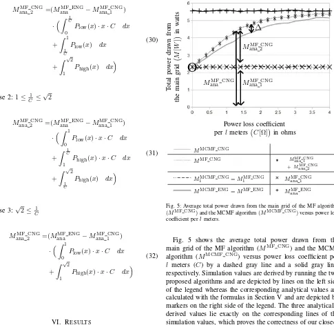
Fig. 5 shows the average total power drawn from the main grid of the MF algorithm (MMF CNG) and the MCMF algorithm (MMCMF CNG) versus power loss coefficient per
l meters (C) by a dashed gray line and a solid gray line, respectively. Simulation values are derived by running the two proposed algorithms and are depicted by lines on the left side of the legend whereas the corresponding analytical values are calculated with the formulas in Section V and are depicted by markers on the right side of the legend. The three analytically derived values lie exactly on the corresponding lines of the simulation values, which proves the correctness of our closed-form expressions in Section V.
The MCMF algorithm saves more grid power than the MF algorithm for any given C >0 because it takes into account the power loss in the transmission lines in the optimization. As a result, the power flow in the network travels over shorter distances in the MCMF algorithm and is therefore subject to a smaller power loss than in the MF algorithm. The performance gap (∆) between the two algorithms is greater for moderate
[image:9.612.71.556.82.553.2]MMF CNG andMMCMF CNG are bounded by the dashed black horizontal lower bound line corresponding to the
MMF CNG
1 = M1MCMF CNG value and the solid black hor-izontal upper bound line corresponding to the MMF ENG =
MMCMF ENG value. The lower and upper bound are hori-zontal lines, because MMF CNG
1 , M1MCMF CNG, MMF ENG, andMMCMF ENGare independent ofC. These two horizontal lines correspond to the extreme points of the cellular network behavior where all BSs behave like one single mega BS corresponding to the dashed black horizontal line in Fig. 5 and all BSs behave like isolated BSs corresponding to the solid black horizontal line in Fig. 5.
The power, which cannot be balanced out in the network and therefore flows on the virtual (s,t)edge, is the same in both algorithms. Hence,M1MF CNGis equal toM1MCMF CNG. The total power drawn from the main grid on an edgeless neighboring graph is the same in both algorithms. Hence,
MMF ENGis equal to MMCMF ENG.
[image:10.612.311.531.82.311.2]B. Different BS Densities
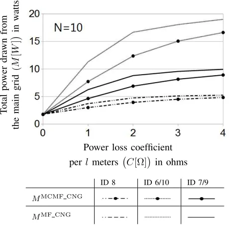
Fig. 6 shows the performance of both algorithms for differ-ent numbers of BSs (N). The performance gap (∆) between the two algorithms increases with the number of BSs, i.e., a denser cellular network. This is because a denser cellular network offers more opportunities for power sharing between BSs, and the power savings from minimizing the distances traveled by the power flows become more significant. The MCMF algorithm saves up to10%,22%and30%more power than the MF algorithm forN = 5,N = 10andN = 15BSs, respectively. The BSs density influences significantly∆.
T
otal
po
wer
dra
wn
from
the
main
grid
M
[
W
]
in
w
atts
Power loss coefficient perl meters C[Ω]in ohms
N= 5 N= 10 N= 15
MMCMF CNG
MMF CNG
Fig. 6: Average total power drawn from the main grid of the two proposed algorithms versus power loss coefficient perlmeters for different number of BSs (N).
C. Different Maximum Power Surpluses/Deficits
T
otal
po
wer
dra
wn
from
the
main
grid
M
[
W
]
in
w
atts
Power loss coefficient perl meters C[Ω]in ohms
B= 4 B= 6 B= 8
MMCMF CNG
MMF CNG
Fig. 7: Average total power drawn from the main grid of the two proposed algorithms versus power loss coefficient perlmeters for different maximum
[image:10.612.48.266.422.648.2]power surpluses/deficits (B).
Fig. 7 shows the performance of both algorithms for differ-ent maximum power surpluses/deficits (B). Greater maximum power surplus/deficit values (B) happen if the maximum power generation rises, e.g., due to solar cells with a greater surface area, and if the maximum power consumption rises, e.g., due to more UEs connected to the BSs. If the B value rises, the average total power drawn from the main grid rises in both algorithms, but the relative performance gap between the two algorithms is constant. In other words, The MCMF algorithm saves up to 22% more power than the MF algorithm for all three cases: B = 4, B = 6 and B = 8. This can be explained by the fact that the power, which cannot be balanced out in the network and therefore flows on the virtual (s,t)
edge, is the same in both algorithms. Hence, MM F CN G
1 is
equal to M1M CM F CN G. The performance gap (∆) between the two algorithms is only caused by the difference between theM2M F CN G value and theM2M CM F CN G value. In other words, the performance gap (∆) is only caused by the fact that the MF algorithm losses more power during the transmission due to longer transmission distances. For the investigated cellular network with N = 10 BSs, the power loss aware MCMF algorithms saves up to 22% more power than the power loss unaware MF algorithm.
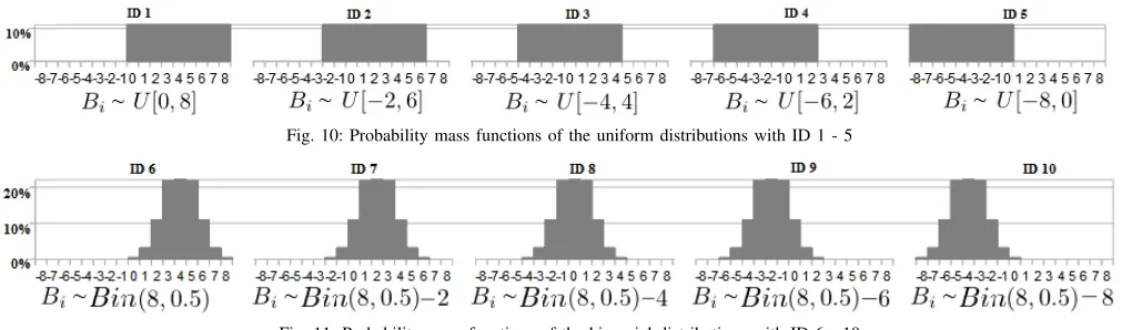
D. Different Power Surplus/Deficit Distributions
We denote the discrete uniform distribution of the integers in the interval [a, b] as U[a, b]. Each integer in the interval is equally likely to be observed. The investigated uniform distributions are given in Fig. 10. The uniform distributions with ID 1, ID 2, ID 3, ID 4, and ID 5 are the uniform distributions U[−4,4] shifted +4, +2, 0, -2, -4 along the x-axis (cf. Fig. 10), respectively.
We denote the binomial distribution with parameters ˜nand
˜
pasBin(˜n,p˜). The probability ofBi having the valuekin a binomial distribution is given as:
P(Bi=k) =
˜ n k
˜
pk(1−p˜)n˜−k k∈ {0,1, ...,n˜}. (33)
The investigated binomial distributions are given in Fig. 11. The binomial distributions with ID 6, ID 7, ID 8, ID 9, and ID 10 are the binomial distributionsBin(8,0.5)shifted 0, -2, -4, -6, -8 along the x-axis (cf. Fig. 11), respectively. We set the parametern˜= 8so that all distributions in Figs. 10 - 11 have the same support. We set the parameter p˜= 0.5 so that the binomial distributions are symmetrical similar to the energy generation profile of a solar cell.
Fig. 8 and Fig. 9 evaluate uniform distributions and binomial distributions, respectively. The absolute values in Fig. 8 are different to the absolute values in Fig. 9 due to the different types of distributions but the general shape of the curves are similar in both figures.
T
otal
po
wer
dra
wn
from
the
main
grid
M
[
W
]
in
w
atts
Power loss coefficient perl meters C[Ω]in ohms
ID 2 ID 3 ID 4 ID 1/5 ID 2/4
MMCMF CNG
[image:11.612.312.542.61.288.2]MMF CNG
Fig. 8: Average total power drawn from the main grid of the two proposed algorithms versus power loss coefficient perlmeters for different distributions
IDs from Fig. 10.
T
otal
po
wer
dra
wn
from
the
main
grid
M
[
W
]
in
w
atts
Power loss coefficient per l meters C[Ω]in ohms
ID 8 ID 6/10 ID 7/9
MMCMF CNG
MMF CNG
Fig. 9: Average total power drawn from the main grid of the two proposed algorithms versus power loss coefficient perlmeters for different distributions IDs from Fig. 11.
1) Different Power Surplus/ Deficit Value Distributions In
One Cellular Network: ID 1/5 and ID 2/4 in Fig. 8 and ID
6/10 and ID 7/9 in Fig. 9 evaluate cellular network scenarios where the power surplus/deficit values Bi do not follow the same distribution among all BSs, i.e., theBi values of half of the BSs follow the first distribution whereas theBi values of the other half of the BSs follow the second distribution.
2) Match/Mismatch Between The Total Power Surplus And
The Total Power Deficit: The slopes of ID 2 and ID 4 are
smaller than the slope of ID 3 in Fig 8. This shows that more power is shared in the cellular network with power distribution ID 3, because the total power surplus and the total power deficit on average is the same for ID 3. BSs with power distributions ID 2 and ID 4 have more likely a power surplus and a power deficit, respectively.
3) High/Low Fluctuations Of The Power Surplus And
Power Deficit Values: ID 1/5 in Fig. 8 and ID 6/10 in Fig. 9
have a high fluctuation of the power surplus and power deficit values. ID 2/4 in Fig. 8 and ID 7/9 in Fig. 9 have a medium fluctuation of the power surplus and power deficit values. ID 3 in Fig. 8 and ID 8 in Fig. 9 have a low fluctuation of the power surplus and power deficit values. The higher the fluctuation the more power is shared in the cellular network and the more power is lost in the transmission lines.
4) Harvesting Devices Are Not Present On All The BSs: ID
[image:11.612.48.291.445.674.2]Fig. 10: Probability mass functions of the uniform distributions with ID 1 - 5
Fig. 11: Probability mass functions of the binomial distributions with ID 6 - 10
5) Different Capacities/Sizes Of Energy Harvesters: ID 1
and ID 2 in Fig. 10 as well as ID 6 and ID 7 in Fig. 11 have a harvesting device of a large size, because it is more likely that these BSs experience a power surplus. ID 3 in Fig. 10 and ID 8 in Fig. 11 have a harvesting device of a medium size, because it is equally likely that these BSs experience a power surplus or deficit. ID 4 and ID 5 in Fig. 10 as well as ID 9 and ID 10 in Fig. 11 have a harvesting device of a small size, because it is more likely that these BSs experience a power deficit.
VII. CONCLUSION
We have developed an MF algorithm and an MCMF al-gorithm to optimize the sharing of renewable power among BSs with the objective of minimizing the total power drawn from the main grid by the BSs. The MCMF algorithm has a higher computational complexity but results in a more efficient use of the harvested power because it minimizes the DDPL in the transmission lines by sharing renewable power among nearby BSs wherever possible. We have derived a closed-form expression of the average total power drawn from the main grid by the BSs for the MF algorithm. Our simulation results on a complete neighboring graph, i.e., every BS can share power with every other BS in the network, have shown that our derived closed-form expression for the MF algorithm is accurate, and that the power saving gain (∆) of the MCMF algorithm over the MF algorithm depends on the power loss coefficient (C) per l (∈R+)meters of transmission line. On the one hand, ∆ converges to0% if C is very large or very small. In such cellular networks, the simpler MF algorithm should be used. On the other hand, for cellular networks with a moderateC,∆increases with the BS density. In such cellular networks, the MCMF algorithm saves up to 10%, 22%, and
30% more main grid power than the MF algorithm for5,10
and15BSs uniformly distributed in a square area ofl2square meters, respectively.
REFERENCES
[1] D. Benda, X. Chu, S. Sun, T. Q. Quek, and A. Buckley, “Modeling and optimization of energy sharing among base stations as a minimum-cost-maximum-flow problem,” inProc. IEEE VTC-Spring, Porto, Portugal, Jun 2018, pp. 1–5.
[2] A. Kwasinski and A. Kwasinski, “Increasing sustainability and resiliency of cellular network infrastructure by harvesting renewable energy,”IEEE Communications Magazine, vol. 53, no. 4, pp. 110–116, Apr 2015. [3] Y. Mao, Y. Luo, J. Zhang, and K. B. Letaief, “Energy harvesting small
cell networks: feasibility, deployment, and operation,”IEEE Communi-cations Magazine, vol. 53, no. 6, pp. 94–101, Jun 2015.
[4] D. Benda, S. Sun, X. Chu, T. Q. S. Quek, and A. Buckley, “PV cell angle optimization for energy generation-consumption matching in a solar powered cellular network,” IEEE Transactions on Green Communications and Networking, vol. 2, no. 1, pp. 40–48, Mar 2018. [5] X. Huang and N. Ansari, “Energy sharing within EH-enabled wireless
communication networks,” IEEE Wireless Communications, vol. 22, no. 3, pp. 144–149, Jun 2015.
[6] Y. Guo, L. Duan, and R. Zhang, “Optimal pricing and load sharing for energy saving with cooperative communications,”IEEE Transactions on Wireless Communications, vol. 15, no. 2, pp. 951–964, Feb 2016. [7] M. J. Farooq, H. Ghazzai, A. Kadri, H. ElSawy, and M. S. Alouini,
“A hybrid energy sharing framework for green cellular networks,”IEEE Transactions on Communications, vol. 65, no. 2, pp. 918–934, Feb 2017. [8] M. J. Farooq, H. Ghazzai, A. Kadri, H. ElSawy, and M. S. Alouini, “En-ergy sharing framework for microgrid-powered cellular base stations,”
IEEE Global Communications Conference, pp. 1–7, Dec 2016. [9] A. F. Crossland, O. H. Anuta, and N. S. Wade, “A socio-technical
approach to increasing the battery lifetime of off-grid photovoltaic systems applied to a case study in Rwanda,”Renewable Energy, vol. 83, pp. 30 – 40, Nov 2015.
[10] Y. K. Chia, S. Sun, and R. Zhang, “Energy cooperation in cellular networks with renewable powered base stations,”IEEE Transactions on Wireless Communications, vol. 13, no. 12, pp. 6996–7010, Dec 2014. [11] CelPlan. (2014) White paper - customer experience optimization in
wire-less networks. [Online]. Available: http://www.celplan.com/resources/ whitepapers/Customer%20Experience%20Optimization%20rev3.pdf [12] R. K. Ahuja, M. Kodialam, A. K. Mishra, and J. B. Orlin,
“Computa-tional investigations of maximum flow algorithms,”European Journal of Operational Research, vol. 97, no. 3, pp. 509–542, Mar 1997. [13] J. Vygen, “On dual minimum cost flow algorithms,” Mathematical
Methods of Operations Research, vol. 56, no. 1, pp. 101–126, Aug 2002. [14] X. Huang, T. Han, and N. Ansari, “Smart grid enabled mobile networks: Jointly optimizing BS operation and power distribution,” IEEE/ACM Transactions on Networking, vol. 25, no. 3, pp. 1832–1845, Jun 2017. [15] H. Cole and D. Sang,Revise AS Physics for AQA A. Oxford, United
Kingdom: Heinemann Educational Publishers, 2001, pp. 67–68. [16] B. Korte and J. Vygen,Combinatorial Optimization: Theory and
Algo-rithms, 5th ed. Germany: Springer-Verlag Berlin Heidelberg, 2012, p. 177.
[17] E. W. Weisstein. (2008) Dice from MathWorld–A Wolfram Web Resource. [Online]. Available: http://mathworld.wolfram.com/Dice.html [18] P. Fan, G. Li, K. Cai, and K. B. Letaief, “On the geometrical char-acteristic of wireless Ad-Hoc networks and its application in network performance analysis,”IEEE Transactions on Wireless Communications, vol. 6, no. 4, pp. 1256–1265, Apr 2007.
[19] Z. Khalid and S. Durrani, “Distance distributions in regular polygons,”
[20] U. B¨asel, “Random chords and point distances in regular polygons,”
Acta Mathematica Universitatis Comenianae, vol. 83, no. 1, pp. 1–18, May 2014.
[21] E. W. Weisstein. (2017) Square Line Picking from MathWorld–A Wolfram Web Resource. [Online]. Available: http://mathworld.wolfram. com/SquareLinePicking.html
Doris Benda (S’17) received the B.Sc. degree in Mathematics from the University of Bonn (Ger-many) in 2014 and the M.Sc. degree from the Liverpool John Moores University (United King-dom) in 2015. Currently, she is pursuing the Ph.D. degree in Electrical Engineering at the University of Sheffield (United Kingdom). Since 2016, she is with the Institute for Infocomm Research (Singapore). Her research interests span various areas in green communication and network optimization, especially the incorporation of renewable energy in the cellular network. She is an awardee of the A*STAR Research Attachment Programme between Singapore and Sheffield.
Xiaoli Chu(M’06-SM’15) is a Reader in the De-partment of Electronic and Electrical Engineering at the University of Sheffield, UK. She received the B.Eng. degree in Electronic and Information Engi-neering from Xi’an Jiao Tong University in 2001 and the Ph.D. degree in Electrical and Electronic Engineering from the Hong Kong University of Sci-ence and Technology in 2005. From 2005 to 2012, she was with the Centre for Telecommunications Research at King’s College London. Xiaoli has co-authored over 100 peer-reviewed journal and confer-ence papers. She is co-recipient of the IEEE Communications Society 2017 Young Author Best Paper Award. She is the lead editor/author of the book “Heterogeneous Cellular Networks - Theory, Simulation and Deployment” published by Cambridge University Press (May 2013) and the book “4G Femtocells: Resource Allocation and Interference Management” published by Springer (November 2013). She is Editor for the IEEE COMMUNICATIONS
LETTERSand the IEEE WIRELESSCOMMUNICATIONSLETTERS. She was Guest Editor for the IEEE TRANSACTIONS ONVEHICULARTECHNOLOGY
and the ACM/Springer Journal of Mobile Networks & Applications. She was Co-Chair of Wireless Communications Symposium for the IEEE International Conference on Communications (ICC) 2015, Workshop Co-Chair for the IEEE International Conference on Green Computing and Communications 2013, and has been Technical Program Committee Co-Chair of 6 workshops on heterogeneous and small cell networks for IEEE ICC, GLOBECOM, WCNC, and PIMRC.
Sumei Sun (F’16) is currently the Head of the Communications and Networks Cluster, Institute for Infocomm Research, Agency for Science, Technol-ogy, and Research, Singapore, focusing on smart communications and networks for robust, QoS/QoE-guaranteed, and energy- and spectrum-efficient con-nectivity for human, machine, and things. She has authored or co-authored over 200 technical papers in prestigious IEEE journals and conferences, and holds 30 granted patents and over 30 pending patent applications, many of which have been licensed to industry. She is a Distinguished Lecturer of the IEEE Vehicular Technology Society 2014-2018, a Distinguished Visiting Fellow of the Royal Academy of Engineering, U.K., in 2014, and Vice Director of IEEE Communications Society Asia Pacific Board since 2016. She has also been actively contributing to organizing IEEE conferences in different roles, including her recent services as Executive Vice Chair of Globecom 2017, Symposium Co-Chair of ICC 2015 and 2016, Track Co-Chair of IEEE VTC 2016 Fall, VTC 2017 Spring, etc. She was an Editor of the IEEE TRANSACTIONS ON VEHICULAR
TECHNOLOGY(TVT) during 2011-2017, and Editor of the IEEE WIRELESS
COMMUNICATIONLETTERSduring 2011-2016. She serves as an Area Editor of IEEE TVT since July 2017, and Editor of the IEEE COMMUNICATIONS
SURVEYS ANDTUTORIALS, since 2015. She received the “Top Associate Editor” award in 2011, 2012, and 2015, all from IEEE TRANSACTIONS ON
VEHICULARTECHNOLOGY.
Tony Q.S. Quek(S’98-M’08-SM’12-F’18) received the B.E. and M.E. degrees in electrical and electron-ics engineering from the Tokyo Institute of Technol-ogy, Tokyo, Japan, in 1998 and 2000, respectively, and the Ph.D. degree in electrical engineering and computer science from the Massachusetts Institute of Technology, Cambridge, MA, USA, in 2008. Currently, he is a tenured Associate Professor with the Singapore University of Technology and Design (SUTD). He also serves as the Acting Head of ISTD Pillar and the Deputy Director of the SUTD-ZJU IDEA. His current research topics include wireless communications and networking, internet-of-things, network intelligence, wireless security, and big data processing.
Dr. Quek has been actively involved in organizing and chairing sessions, and has served as a member of the Technical Program Committee as well as symposium chairs in a number of international conferences. He is currently an elected member of IEEE Signal Processing Society SPCOM Technical Committee. He was an Executive Editorial Committee Member for the IEEE TRANSACTIONS ON WIRELESS COMMUNICATIONS, an Editor for the IEEE TRANSACTIONS ONCOMMUNICATIONS, and an Editor for the IEEE WIRELESS COMMUNICATIONS LETTERS. He is a co-author of the book “Small Cell Networks: Deployment, PHY Techniques, and Resource Allocation” published by Cambridge University Press in 2013 and the book “Cloud Radio Access Networks: Principles, Technologies, and Applications” by Cambridge University Press in 2017.
Dr. Quek was honored with the 2008 Philip Yeo Prize for Outstanding Achievement in Research, the IEEE Globecom 2010 Best Paper Award, the 2012 IEEE William R. Bennett Prize, the 2015 SUTD Outstanding Education Awards – Excellence in Research, the 2016 IEEE Signal Processing Society Young Author Best Paper Award, the 2017 CTTC Early Achievement Award, the 2017 IEEE ComSoc AP Outstanding Paper Award, and the 2017 Clarivate Analytics Highly Cited Researcher. He is a Distinguished Lecturer of the IEEE Communications Society and a Fellow of IEEE.