Department of Forestry
Australian National University
Mathematical Programming for Advanced Forest Management Planning in Fiji
Optimising Harvest Wood Allocation in the Mixed-hardwood Plantations using Linear Programming Model
by
Osea Tuinivanua March 1991
Acknowledgements
I wish to express my sincere appreciation and gratitude to the many individuals and organisations who contributed to the completion of my study.
My special thanks to the German Agency for Technical Cooperation (GTZ) and the German Academic Exchange Service (DAAD) for their sponsorship, given under the Fiji German Forestry Project, Fiji. I also thank the Fiji Government for granting me an opportunity for further studies.
A very sincere and special thanks to my supervisor, Dr B. J. Turner. His support, patience and guidance offered many meaningful directions in the course of my study, especially the concept of advanced forest management planning, its application in developing countries and the completion of my subthesis. I also thank my good friends : Gary Richards and Patrick Milimo for their editing work ; and Joe Miles for his invaluable assistance in the understanding and application of computers.
Abstract
Short to long term forest management planning of native forests and forest plantations in many developing countries has proven a difficult undertaking. Beside the inherent social difficulties relating to land tenure, there are always inadequate personnel and limited relevant resources to carry out appropriate planning for wood and non-wood demands with the changing market scenarios. Adoption of appropriate decision support systems from countries where they have been successfully used may resolve some of the uprising conflicting demands on our forest resources.
TABLE OF CONTENTS
I V
Acknowledgements Abstract
Table of Contents List of Tables List of Figures
1. Introduction 1
1.1. Forest Planning Process - Fiji Forestry Department 3
1.2. Objectives of the study 5
2. Development of Forest Planning Processes in Other Countries 7 2.1. Why the USDA Forest Service and Australia ? 7
2.2. USDA Forest Service 8
2.3. Australian State Forests Planning 13
2.4. Linear Programming Models as Analytic Tools 16
3. Development of Mathematical Programming for Forest Management Planning 18
3.1. The Emergence of Mathematical Programming 18
3.2. Single Objective Approach of Forest Management Planning 20
3.2.1. Development of Linear Programming 20
3.2.2. Scientific Management Approach using Linear Programming 28 3.3. Multiple Objectives Approach of Forest Management Planning 36
3.3.1. Goal Programming 36
3.3.2. Application of Linear Goal Programming 41
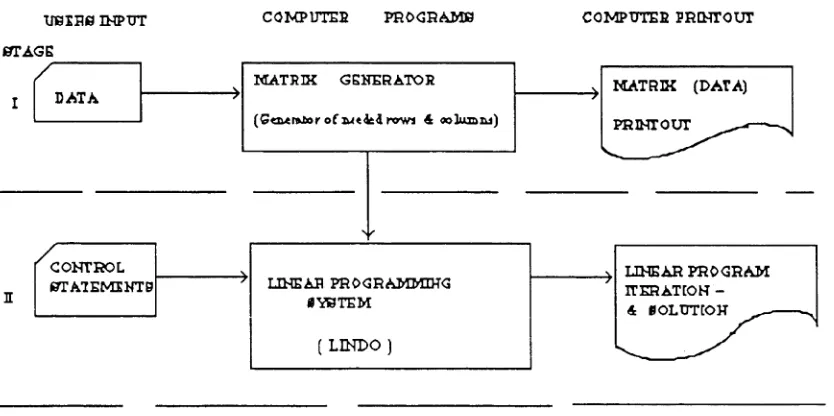
4. Methodology of Scheduling Problem with the SCHEDULER System 43
4.1. Introduction 43
4.2. System Configuration 44
4.3. Stages of Scheduling Process 49
4.3.1. Data Input 49
4.3.2. Control Statements 50
4.3.3. Matrix Generation 51
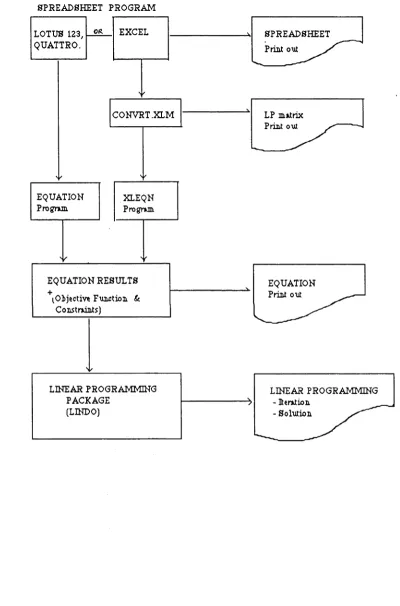
4.3.3.1. Pre-made spreadsheet 51
4.3.3.2. Formating own spreadsheet 51
4.3.3.3. Primary Data Section 53
4.3.3.4. Linear Program Matrix Section 54
V
4.3.5. Linear Program Solution Output 59
5. The Study Region : Fiji Forestry Sector 61
5.1. Background Information 61
5.1.1. Location and Geographical Features 61
5.1.2. Climate 61
5.1.3. Soil and Geology 62
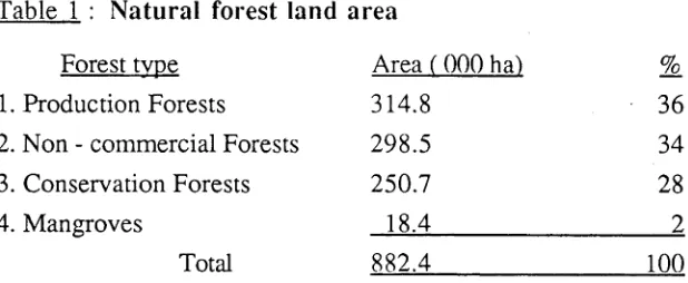
5.1.4. Natural Vegetation 63
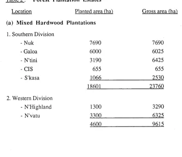
5.1.5. Forest Plantations 65
5.1.6. Land Tenure 69
5.1.7. Land Capability and Land Use Pattem 70
5.1.8. Population and Employment 74
5.2. F iji Forestry Sector 75
5.2.1. Forestry Department 75
5.2.2. Forestry Sector Planning Process 79
5.3. F iji Timber Industries 81
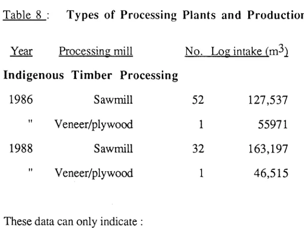
5.3.1. Wood Processing Sector 81
5.3.2. Logging Industry 84
6. Case Study : Mixed-hardwood Plantations 86
6.1. Introduction 86
6.2. Forest Resource 87
6.3. Forestry Growth and Yield Model 89
6.4. Problem and Problem Formulation 91
6.4.1. Problem Formulation 95
6.4.2. Mixed-hardwood Model 98
6.5. Management Alternatives 100
6.5.1. Case 1 : Non-declining flow to integrated mills 101
6.5.2. Case 2 : Non-declining flow to integrated and sawmills 101 6.5.3. Case 3 : Non-declining flow with increasing harvest areas 102
6.5.4. Case 4 : Sensitivity o f PNV to Rotation Ages 102
7. Results and Discussions 103
7.1. Case 1 104
7.2. Case 2 107
7.3. Case 3 110
7.4. Case 4 112
8. C o n c l u s i o n s 121
8 .1 . R e c o m m e n d a t i o n s 123
8 .2 . F u r t h e r w o r k 124
R eferen ces
List of tables
1. Native Forest Area 64
2. Forest Plantation Estates 65
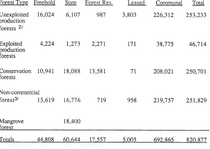
3. Land Ownership by Forest Type and Area 70
4. Land Capability for Agriculture and Plantation Forestry in Fiji 71
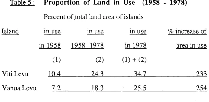
5. Proportion of Land in Use (1958 - 1978) 72
6. Proportion of Land with Slopes > 18° ^
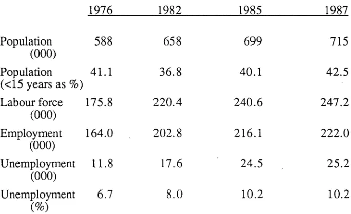
7. Population and Employment 75
8. Type of Processing Plant and Production 82
9. Area / Age - Class Distribution and Planning Process 89
10. Yield per Harvest Area for the 5 and 25 years 93
11. Processing Centre Gate Prices of Peeler and Sawlogs 94
12. Area Control for harvesting per Cutting Period 95
13. (a) Area allocation per harvest area in the 5 year Cutting Period 104
(b) Distribution of harvest area (%) per Processing Centre 105
14. (a) Volume of Product Assortments harvested in the 5 year Cutting Period 105
(b) Cost and Revenue Estimates for 5 year Cutting Period 105
15. (a) Area allocation per harvest area to each Processing Centre 107
(b) Volume of Product Assortments 108
(b) Cost and Revenue Estimates for the 5 year Cutting Period 108
16. (a) Area allocation per harvest area for the 3 year Cutting Period 110
(b) Volume of Product Assortments harvested 110
(c) Cost and Revenue Estimates - Case 3. I l l
17. (a) Harvest area - Case 4. 113
(b) Harvest volume - Case 4. 113
(c) PNV - Case 4. 115
V
List of Figures
1. LP Approach with The SCHEDULER System 46
2. The SCHEDULER System 48
3. Alternative A : Pre - made Spreadsheet 52
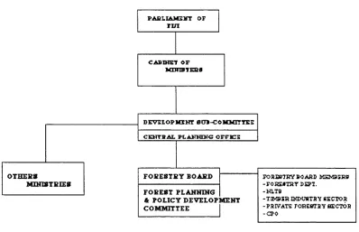
4. Fiji Forest Sector Policy Development & Planning Process 80
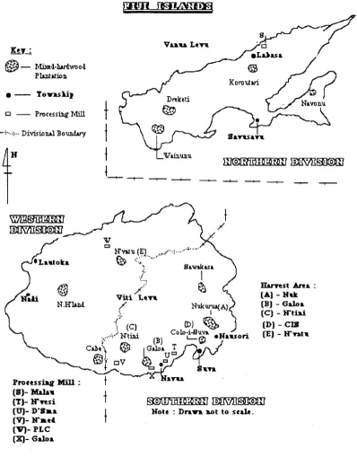
5. Distribution of the Case Study Harvest Area 88
6. Net Revenue: Case 4. 114
7. PNV : Case 4. 115
8. PNV : Cases 1 and 2. 119
9. Logging and Hauling Costs : Cases 1 and 2 119
10. Net Revenue : Cases 1 and 2 119
Appendi ces
1. (a) Case 1 Sample Spreadsheet with Formulas 131
(b) Case 1 Sample Spreadsheet with LP Matrix and Primary Data 132
Chapter 1
1. INTRODUCTION
The myth that “trees are renewable” has little or no meaning to most rural dwellers in the Fiji Islands. Local trees and native forests are part of their ancestral heritage to provide basic necessities for the current and coming generations. Blessed by the abundant forests, so it seemed, most landowners have exploited their forests as an alternative source of income, only to realise that the outcomes have made them worse off. O ther landowners acknowledged their forests as nothing but a hindrance to their subsistence farming and agricultural development.
The combined effect of these two motives have contributed significantly to the rapid decline in forest cover. With less than 50% (855,000 ha ) of the total land area under forest in late 1950’s, the Forestry Department was enacted to established two reforestation programs.
This study represents the introduction of M anagement Science, in particular, mathem atical programming (MP), into forest management planning in Fiji and the decision making associated with man-made mixed-hardwood plantations. Initially, this would require the identification of a suitable mathematical programming technique to assist in selecting optim al forest managem ent strategies and activities to satisfy management goals and objectives.
In the case study, mathematical programming was used to investigate certain single and multiple-use objectives of forest management. In addition, appropriate management strategies for the next two to three decades were identified. The study was not intended to absolutely resolve the problems of forest management or dictate the decisions to be taken. It is essentially a comprehensive evaluation of selected mathematical programming models and their technical and economic efficiency as working tools.
In the study, a system of computer programs called the SCHEDULER System, developed by Schurr and Davis (1989) was used. The SCHEDULER System is designed to optimise management objectives within economical and physical constraints with a linear programming package (LINDO) and additional software. Two techniques, linear programming for single objective and goal programming for multiple objectives, and their solution process have been investigated.
Linear programming models form an integral part of advanced forest management planning models in the USDA Forest Service and some Australian state forestry services, even as concepts of forest planning have shifted from functional analysis to multidisciplinary and integrated forest management planning. Fiji forest management decision making can no longer rely on the old and inept planning process. The Forestry Department needs to develop and implement some scientific management techniques, taking advantage of advanced technology developed by the USDA Forest Service and in Australia.
1.1. Forest planning process - Fiji Forestry Department
The Fiji Forestry Departm ent is not required by law to produce forest management plans for plantations under its jurisdiction, nor for native rainforests that it jointly supervises with the Native Land Trust Board (NLTB) for landowners. The forest planning process is at present too fragmented and inefficient to meet the industrial and environmental requirements entrusted upon the Forestry Department. Forest management decision making is too centralised, restrained by limited expertise in most forest disciplines, constrained by minimal budget, and suffers from undefined management priorities with unclarified goals.
seen as a competitive land user and viewed with scepticism since its inception in 1913. In recent years, every action it took, or did not take, prompted either public criticisms or landowners discontent, indicating that the Forestry Department is not effectively managing the problems at hand.
Surprisingly, the colonial system of "one-way communication" of forest policy and instructions from "top-to-bottom" had worked, resulting in the accomplishment of timber self-sufficiency in 1974 and the partial fulfilment of targeted reforestation program of grasslands (60,000 ha) and logged over rainforests (100,000 ha) (Fiji Govt., 1985). In the last five decades, the forest management was largely timber oriented, based on tim ber com m itm ent to industries, and availability and accessibility of resources. Technically based decisions were scarce or cleverly disguised, as decisions were often individually or politically motivated and based on experiences from other countries.
A modified and rational approach to forest management is critical in Fiji, to assist decision making that could stabilise the fragile environment and economy (Drysdale, 1988; FFD, 1988; Tuyll and Tuinivanua, 1988). The needed approach should promote multidisciplinary and integrated planning toward multiple-use management (Drysdale, 1988). Forest planning processes should take advantage of advanced technology, e.g., com puterised technology and other mathematical programming techniques (linear programming models) as analytic tools to assist the decision making. An appropriate forest resource planning hierarchy could be portrayed as fo llo w s:
1. National Forest Planning :
underdeveloped (Westoby, 1989). Realising these features, NFP must have, if possible a quantified concept of its future place in dom estic and international markets and timber economy. The planning should have some notion o f the extent to which it intends or expects the forest resources to contribute to timber and non-timber needs.
2. Divisional Forest Planning :
Divisional Planning (DP) would be responsible for translating forest policy and objectives into prescription plans. To achieve this, appropriate planning and analytic tools must be devised. Quite often, DP provides an essential link, ensuring efficient connection between management plan at the divisional and station levels to the National Plan. Examples of DP would include a production plan that defines the supply of wood to existing wood processing mills; recreation plan; and protection plan for water catchments, wildlife and other reserves.
Most importantly, Divisional level planning would not only decentralise responsibility of management planning but also enhance decision making for divisional and station managers. These plans should be flexible, accessible to all staff, practical and easily understood by users, and capable of analysing and producing realistic solutions.
1.2. Objectives of the Study
1. Test and evaluate the feasibility of the SCHEDULER System as :
(a) an appropriate harvest wood allocation system for the mixed- hardwood plantations of the Fiji Forestry Department.
(b) a useful tool for advanced forest management planning process.
(c) an efficient decision support system.
Given the primary is satisfied, success of the study would :
1. Create an awareness for advanced forest planning techniques, thus providing better insights into forest management problems and the required information technology for the system to produce quality results.
2. Replace the 'ad hoc' decision making based on haphazard planning and make scientific forest management techniques an integral part of planning processes.
3. Adopt a modified or transformed advanced technology : com puterised mathematical programming techniques, e.g., LP models that coincide with the budget level, staff, quality and quantity data and the value of forest resources being analysed.
4. Intensify advanced forest management planning at all divisional and station levels.
Chapter 2
2. DEVELOPMENT OF FOREST PLANNING PROCESS IN OTHER
COUNTRIES
2.1.
Whv the USDA FS and Australia ?
Fiji can no longer regard its forest economy a closed one. The country's self-
reliance reached two decades ago, and now, the exportable surplus from the native
forests and plantations has forced the national planners to develop ways that ensure the
optimum economic utilisation of the forest resource. Yet, Fiji's forest management
planning is at its juvenile stage. The reality is that, the Fiji forest management is
technically backward and falls far behind its developed neighbours. Fiji needs to
outwardly research their forestry development and planning to avoid flaws of the past
and keep pace with the modem forestry development.
The USDA Forest Service and Australian State Forestry Services have made
professional approaches to their forest management in the early and mid-1900's
respectively. Interestingly enough, their forestry development have gone through similar
changes from the single objective to the conflicting multiple-use management planning
and the decision support system to optimise these objectives. The increasing and
conflicting public demands on Fiji's forest resources are no different from that
experienced in neighbouring countries. So, by gaining a better understanding of their
systematic approach to solution method techniques would not only promote the
introduction of advanced management planning techniques, but most importantly,
2.2. United States Department of Agriculture-Forest Service (USDA FS)
After Congress passed the Organic Act of 1897 and Transfer Act of 1905, the
USDA Forest Service was established as the governing agency of the National Forests.
These are comprised of 191 million acres ( 77.3 million hectares) of forest land with
annual estimated production of 12 million board feet of timber, 10 million animal unit
months (AUM) of grazing, and many other products, such as recreation opportunities
(Iverson and Alston, 1986). Over eight decades, the USDA Forest Service has evolved
from custodial protection and conservation of these national forests to intensively
integrated management at an unprecedented scale.
Forest planning is an ancient art. Germany had long been managing its forests on a
sustainable basis. This had influenced the USDA Forest Service planning process as well
as the underlying ideology (Alston, 1983). However, Gifford Pinchot, Chief of USDA
Forest Service, 1898, not only spelled out the necessity of multiple-use planning, but
also advocated "that forest conservation should include wise use and, when appropriate,
protection from overuse as well as long term preservation of the productivity of forest
reserves was to be implemented through planning" (Iverson and Alston, 1986). A
professional approach to forest management, recognising the many uses of forests other
than just timber production was the only alternative for managing the new Forest
Service's 85.6 million acres ( 34.6 million ha.) of national forests in 1905 (Alston,
1983).
The concept of multiple-use was later broadened from the commodity use of
forests to include outdoor recreation, wildlife habitat, environmental amenities and
aesthetics (Alston, 1983). Similarly, planning emphasis also shifted from local and forest
level to that of national issues. It called for more flexible multi-purpose management
planning process that reflected not only the national economic conditions but also
prepared for changes to cope with community stability and employment opportunities
The advent of World War II had tested the national forest management plans, proving them to be largely academic. These management plans were for resources that nobody wanted. Instead, their forest supply was drawn from the abundant old-growth timber of private, commercial and industrial forests at lower costs (Behan, 1967, 1981). Demands for forest produce for housing and construction work continued to soar, making the raw materials in the forest reserve a prime target. However, only 45% of forest area of the USDA Forest Service had been roughly surveyed and inventoried, with less than half the inventory data collected been analysed. The basic land classification scheme used for inventory and timber planning was questioned by studies of Wikstrom and Hutchison (1971), who showed the estimates were not complete, lacking important factors such as accessibility, difficulties of regeneration and soil stability measures.
The postw ar period between 1945 and 1960 saw the reshaping of forest management planning in reaction to experiences that previous concepts were too academic. Gross (1950) commented that many of the formulas developed were highly theoretical. Nevertheless, they paved the way for timber activities and harvest schedules that could answer when, where, how and how much timber to cut and regenerate to achieve the management objectives. For example, Area and Volume Control methods were used to regulate the allowable cut. With Area Control, the emphasis was on an annual cut of equal area. Volume Control was focussed on providing an equal volume to harvest annually. The search for more flexible formula identified the Hanzlik's formula17 that was quite popular from 1920's, and well into the 1950's. The Hanzlik method was able to regulate the cut and to permit the rate of harvest to exceed growth where old growth virgin forests predominated. But the search continued, looking for better rotation length, best management practices and best alternative strategies.
17 Annual cut = (Vm)/R +1
where R = rotation length for young growth stand Vm = volume of merchantable (old growth) timber
The 1900 to 1950 era saw an end to custodial management of forest resources (Clawson, 1983), where protection and preservation of forest resources had to undergo inevitable changes towards intensive forest management. The 1960's and 1970's period marked the recovery of the housing and construction industry, accompanied by increase in demand for timber and other uses of forest resources. Favourable stumpage rates had boosted timber harvesting throughout the country, prompting public foresters to reveal a pessimistic view of timber famine. This pessimism was based on inadequate data. Reappraisal has indicated the estimated allowable cut was based on over-estimated, over- optimistic assumptions of the amount of growth on forested land being available and economically feasible to harvest (Duerr, 1960).
The pressure for increased harvest was accompanied by rising demands for other outputs and resources of the National Forests (Craft, 1970). The increasingly competitive users led to the introduction of the Multiple Use Sustained Yield (MU-SY) Act 1960, attempting to balance the demands and services on the Forest Reserves (Alston, 1972; Craft, 1970), and a series of studies on timber supply problems. However, it was the notion of "allowable cut effect" of Multiple Use Sustained Yield that became the focal point of debate (Bell et al., 1975; Teeguarden, 1973; Hyde, 1980). It led to the development of Timber Resource Economic Estimation System (TREES) which used a binary search algorithm to analyse the future timber availability in Oregon (Johnson and Tedder, 1983). Fight et al (1979) discounted the notion that the allowable cut effect was the main constraint, but found constraints on protecting water quality, recreation values, and wildlife habitats were so severe that they could vastly influence the timber program optimisation.
were integrated with plans for other functional areas into the m ultiple-use plans (Chappelle et al., 1976; Iverson and Alston, 1986). The desire was to construct models that could look beyond the current rotation and also provide estimates of expected harvest and growth relationships to the future. It required more detail information, not only of resources but also activities to be applied. The attempt was faced with two problems: estim ation of existing inventory and its growth and yield models and secondly, translation of information into an allowable cut estimate. With the sophisticated computer models in use, the USDA Forest Service continued its timber scheduling beyond the current rotation but were restricted as resource interactions could not be modeled effectively. This was important as the MU-SY Act 1960, the National Environmental Protection Act (NEPA) 1969, and the National Forest Management Act (NRMA) - 1976, were emphasising a shift from single objective to multidisciplinary and interdisciplinary planning (Iverson and Alston, 1986).
oriented concept followed by the strengthening of local or regional level planning. In other words, the shift in the mode of planning was made toward decentralising the forest management planning process.
With the MU-SY Act of 1960, emphasis shifted toward a balanced approach in the use and management of forests and range lands (Alston, 1972). Nevertheless, no matter how far the intention was to recognise the balanced approach, the absence of adequate data and expertise in non-timber planning had resulted in multiple-use plans that were still largely timber oriented (Schweitzer and Cortner, 1984).
In response to the National Environmental Policy Act (NEPA) - 1969, requiring all agencies to prepare Environmental Impact Statement (EIS), the USDA FS restructured its system of forest planning. Each forest is divided into subareas of forest called "units," encompassing forest zones, watershed, recreation, streamlines, wildlife habitats and other critical zones. The multiple-use plan would be prepared for all forest components, giving interdisciplinary and / or integrated plans of national forests. However, the functional plan would continue to supplement the overall decision concerning forest resource management. National level planning was becoming the main concern of the general Forest Service planning effort. For example, national level analysis would determine the form and extent of budget allocations to National Forests and Regions.
Eventually, this lead to the formulation of the F O R est P L A N ning Model (FORPLAN), a primary analysis tool providing a link between functional resource planning and integrated land-use planning (Kelly et al., 1986; Johnson, 1986). FORPLAN was com prehended as an analytic tool for developing forest ecosystem management plans or capable of accommodating both land and water in the forests, a role that Timber RAM and MUSYC could not fully handle. Refinement of FORPLAN in Version 2 enabled each discipline to be redefined as a focal point, giving each discipline equal opportunity.
Like most former models and its predecessors, FORPLAN uses a mathematical programming technique especially linear programming, classifying it as linear model. FORPLAN intends to overcom e the short comings of previous models, but certain criticisms are leveled at its inability to handle non-linear problems. The extent of the model can be very complex and sophisticated to provide a clear insight into the planning process. However, mathematical programming such as linear programming, provides a useful mechanism in understanding the nature of the problems.
2.3. Australian States Forest Planning.
The extent and type of forest planning varies between States and is largely determined by the data required and available. For example, data from natural hardwood forests are scarce and because of its slow growth and low value, detailed planning and modeling is limited (Australian Forestry Council, 1987). On the other hand, Australia had over a century of experience with industrial plantations of fast growing, exotic species like Pinus radiata. The extensive inventory and growth and yield data collected over the years, enabled the formulation of simulation models and optimisation.
(Turner et al., 1977), - South Australia (Ferguson et al., 1978); STANDS1M- general model for sim ulating growth of even-aged stands - Victoria (Opie 1972). Simulation models of growth and yield saw the move to more advanced form of analysis, e.g., using linear regression with computer modeling replacing graphical analysis. Simulations for cutting plans and yield regulations schedule the types of thinning operations and clearfelling for 1 - 5 years and yield regulations for 20 - 60 years. These simulation models are product oriented to satisfy the industries. The objectives behind these models were ease of use, cost effectiveness and ability to take advantage of computer technology. Examples of cutting plans include: Plantation Simulation Model 1 (PSM) - Cutting Plan, using stand growth model -Victoria (Dargavel et al., 1976); PSM 2 - Cutting Plan, using linear regression - South Australia (Lewis et al., 1976); PSM 4 - Yield Regulation, using yield table projection - Victoria (Dargavel, 1969); PSM 5 - Yield Regulation, yield table projection - South Australia (Lewis et al., 1976); PSM 7 - Yield Regulation - FORSIM, growth simulation based on basal area, height and simulation of harvesting operation - Victoria (Gibson et al., 1971). The extent and complexity of models vary considerably depending on variation of sites and the decision used for selection (Australian Forestry Council, 1978). A common weakness of the simulation models had been the limited range of management strategies as the complexity of models increased (Lewis et al., 1976; Dargavel, 1969)
The optimisation models for yield regulation represent the introduction of the linear programming model into forest management planning. Linear Programming models
(1971)
developed by Ware e t a 1 , and Johnson and Scheurman (1977), provided the software packages for analysis. Optimisation models that were developed include : the RADiata Harvesting Operation (RADHOP) - NSW \ (B rack , 1988) ; and MASH for the modeling of Eucalyptus regnans and E. delegatensis regrowths - Victoria (Weir,
A balanced approach to multiple use management and integrated planning of native hardwood forests was pursued in Australia, especially in Victoria (Victorian Govt., 1986). Growing confrontations between practitioners of forest m anagem ent and environmentalists had intensified over the years (Church, 1987). Similarities in the problem scenario between the United States and Australia has instigated the Otway Project using FORPLAN (Dargavel and Turner, 1989; Duguid et ah, 1990). In the Victorian context, the Otway model is to resolve some forest management problems, viz.:
(1) how to set the level of the various commitments such as timber production and water supply.
(2) how to manage the forests to meet these commitments
(3) how to ensure that all other uses and values of the forest such as recreation and conservation can be sustained (Duguid et al., 1990)
The development of FORPLAN for the Otway Project can assist the decision making process of the Department of Conservation and Environment of Victorian Government in many ways including :
(1) providing a clear presentation of the planning problem
(2) highlighting missing information during the process of development
(3) testing of flexibility by applying ranges of management alternatives
(4) analysis of responses to different management alternatives
(5) examination of conflicting interactions between multiple uses
(6) quantification of the impacts of management alternatives
- prescriptions to produce goods, services and benefits for the plan period
(8) highlighting poorly defined information critical to good management for further inventory or research (Duguid and Dargavel, 1988)
Although FORPLAN provides potential advances in modern planning model, its many deficiencies are yet to be overcome to become user friendly.
2.4. Linear Programming Models as Analytic Tools
The above review suggests the evolution of the planning process from the functional analysis of Timber RAM to a multidisciplinary and integrated planning method using FORPLAN. Linear Programming is a mathematical programming technique that provides the mechanism to schedule specific management activities of alternative management strategies. It enables the comparison of alternative management strategies to achieve stated goals within limitations of resource.
Chapter 3
3. DEVELOPMENT OF MATHEMATICAL PROGRAMMING FOR FOREST MANAGEMENT PLANNING
3.1. The Emergence of Mathematical Programming
Management Science or Operations Research is a hybrid science with origins
ranging from mathematics, physics, statistics, economics and other applied sciences
(Thompson, 1967). Giving a precise definition of Management Science may be rather
difficult, which is not surprising, because it is simply what management scientists do
(Dykstra, 1984). For convenience, Wagner (1969) defined Management Science as :
A scientific approach to problem solving for executive management"
by using Management Science applications involving :
- "constructing mathematical, economical and statistical descriptions or models of decisions to treat situations of complexity and uncertainty.
- analysing the relationships that determine the probable consequences of decision choices.
devising appropriate measures of effectiveness to evaluate the relative merits of alternative actions"
Management Science is concerned with scientific management, or in other words,
the applications of scientific methods to management of organisations or systems
(Dykstra, 1984). Management Science was developed during World War II to study and
develop solution methods, and how efficient decisions could be reached. In studying
solution methods, the importance of model building was a matter that could not be
overlooked. Model building requires the specialised skills of model developers. As a
result, most of the models that have been devised were largely tailor-made for specific
of a real management problem (Wagner, 1969). It must have sufficient detailed
information to provide a solution that is realistic. Reaching a realistic solution is not an
easy task, thus making model building difficult and strenuous work for model
developers.
Mathematical Programming is a subdiscipline of Management Science (Dantzig,
1963
;Dykstra, 1984
).It represents a class of mathematical techniques that, from time to
time, proved to be a powerful and effective approach to solving real management
problems (Hall, 1967
).To optimise (maximise or minimise) the value of a stated
objective under a set of constraints, mathematical programming is set to follow a defined
procedure called an " algorithm.” A successful algorithm improves and reduces the
number of iterations while ensuring that the optimal solution is not overlooked. The most
developed of these techniques is linear programming. Despite its wide use, linear
programming models have their limitations. Other techniques that were developed
because of the inability of linear programming models to handle other management
problems include : integer, quadratic and dynamic programming.
Mathematical programming in most contexts is concerned with the optimal
allocation of scarce resources to competitive users. Multidisciplinary and integrated
planning have been recognised as potential means of assisting decisions on conflicting
demands and values on forest resources. The efforts to use mathematical programming in
real scheduling problems highlighted some unresolved difficulties of the LP model. But
the mathematical programming techniques have provided greater insights into real
management problems, in particular, the social, economical and biological issues(Ware
and Clutter, 1971
;Hall, 1967
;Dykstra, 1984
).The departure of the planning process from the concept of traditionally regulated
(normal forest) forests was inevitable, especially with its inflexibility and inability to
management alternatives being made available by mathematical programming techniques. With mathematical programming modeling it was possible to evaluate a wide range of resource allocations and scheduling that was never thought possible (Wagner, 1969). In particular, linear programming provided a breakthrough in amplifying the analytic ability of management to decide the best alternative (Wagner, 1969; Ware and Clutter, 1971; Johnson and Tedder, 1983).
3.2 Single Objective Approach of Forest Management Planning
3.2.1. Development of Linear Programming Technique
Linear Program m ing is a discipline of M anagem ent Science which uses mathematical programming techniques. Linear Programming (LP) has a number of
origins : Game Theory ; Input-output Analysis ; and
the Transport Problem . Dantzig (1947) developed the Linear Programming approach to solving scientific management problems. Linear programming
is widely accepted as a scheduling and assignment technique. It optimises (maximises or minimises) the allocation of resources according to a stated linear objective function by satisfying a set of linear constraints.
Curtis (1962) described how LP was perceived and defined by some scientists :
(1) ‘‘Linear Programming is a technique for specifying how to use limited
(2) “Linear Programming is concerned with the problem of planning a complex of interdependent activities in the best possible optimal fashion”
Linear Programming represents a quantitative analysis of management problems. A
prelude to a quantitative analysis requires a thorough understanding of the decision
problem (see Study Area and Case Study). Having a preliminary notion of : principal
management decisions and measure of effectiveness of choices (objectives); marginal
usage of each resource (constraints); and comparisons of alternatives (sensitivity
analysis) are prerequisites that pave the way for a better appreciation of the problem and
decisions to be made (Wagner, 1969; Dantzig,1963). To be classified under LP, a
number of assumptions must be satisfied. These assumptions delineate the limits of LP,
making it computationally possible to achieve a better insight within the decision
problem:
1. Linearity :
Essentially, the objective function and constraints have to be linear throughout the
process of each activity. For example, all constraints must remain as first - degree
polynomials. Strictly speaking, all variables must have exponents of 1. Assumptions of
linearity appear more restrictive than they are in actual use in the processing of each
activity.
2. Proportionality :
It requires that the quantity of flow of various items into and out of the activity is
always proportional. For example, to double mill volume intake would mean doubling of
3. Non-negativity :
An activity can only operate with positive numbers or quantity. Negative numbers or quantities of activities are neither possible nor workable under this condition.
4. Additivity / Divisibility :
Assumptions of additivity and divisibility imply that the LP model is formulated under terms of linear relations. Each variable can assume any real value, integer or continuous.
Formulating a LP model requires an understanding of the decision problem that provides information input under these fundamental stages :
1. Objective :
An objective represents the desire of the decision maker. It optimises one aspect of the decision problem. For example, a forest management goal may be to maximise the utility of forest resource in profits (measured in present net value (PNV), return on investment or maximum wood flow). Other non profit objectives including minimising cost and maximising the timber volume production.
2. Goals and Constraints :
role in multiple objectives approaches. Common forms of goals and constraints include : maximum mill requirements, maximum area and volume of wood flow, budget, or labour supply.
Given its pragmatic considerations, current management decisions should not be restricted by long term objectives. Uncertainty in wood requirements, prices, costs, markets and technology can change future scenarios. Therefore a proper basis for the management of a profit oriented enterprise is to optimise (maximise) its present net value subject to constraining environmental factors. For non profit oriented management, achievements of balanced use may prove more complex to formulate and implement.
3. Problem Formulation :
The establishment of a baseline mathematical model is a key part of the first phase of model formulation (Wagner, 1969; Ignizio, 1982).
Model Formulation
The attempt to identify and mathematically define decision or control variables, objectives, goals and constraints that best describe the decision problem can take the following basic steps:
1. Determination of Decision (Control) Variables
The decision variables are those variables that we can actually control, sometimes referred to as control variables.
2. Formulation of Objectives and Goals
The objectives and goals can be determined by looking at the following/: - Aspirations (desires) of decision makers
- State of resources (limiting)
The distinction among objectives and goals in the context of the problem
formulation can be defined as follows :
(a) Objectives are represented by mathematical functions of the decision variables,
expressing the desires of the decision maker such as maximising PNV or minimising
cost. In linear form, the objective function is linear with the right hand side of the
objective function left unspecified.
maximise
f(x)
or minimise
f(x)
(b) A Goal is a mathematical function of the decision variables that represent the
combination of the objective and a target value.
/ (x) >, < or - b.
A linear programming problem can be written in a number of ways. For example,
the objective function may be maximised or minimised, constraints may be in either
direction of inequalities ( > or < ) and equality (=).
Objective :
Max. (Min.) = C[ xj + C2 X2 + ... + cn xn
where
c
i ^c n are constant parameters. Each parameter cj measures the
contribution of corresponding variable xj to the objective function
Goal or Rigid Constraints :
Subject to :
a l , l x l + a l ,2 x2 + ...+ a l,n xn ( * ) b l
a m ,l X1 + a m2,2x 2 + + a m , n x n (* ) b m
where x > 0
and t>i b 2 ... ,bm are constants. It m easures the amount of resources available, e.g., area, budget, etc., and the expression (*) is either type I inequality ( < ) or a type II inequality ( > ) or an equality for each 1,...,m. Therefore a y is a constant that measures how much of resource T is used per unit of activity xj For example, product a y is the amount of resource T used when activity *j* is at level xj. Addition of these products (activities ) leads to the general expression for total amount of resource T used by 'n' activities. The standard form can be written in somewhat more compact form given : xj (j = 1,...,n ).
Objective function :
n
Max. Z = X cj \j
j = l
Constraints :
subject to
n
X a i j xj < b[ for i = 1,... ,m. j= l
xj > 0 for j = 1,... ,n.
Solving Linear Programming Problems
over and over again called an "algorithm." This particular algorithm for solving LP problems is called the "Simplex Method."
Simplex Method
Dantzig (1963) developed the Simplex Method in 1947. It’s an algorithm for computing numerical solutions to linear programming problems. So, after decades of computational experience, Dantzig became convinced that the Simplex Method was an "efficient" algorithm , meaning that it could quickly find the optimal solution to a LP problem irrespective of problem size. In other words, the simplex algorithm can determine the optimal solution by evaluating only a fraction of the total number of basic solutions.
Slack variables
In solving LP problems via the simplex algorithm, it is essential that type I and II inequalities are converted to equalities in the linear equations. The conversion of inequalities into equality linear equations requires the addition of non-negative variables to the left hand side called slack variables. The slack variables represent a measure of the amount of slack or unused resources in the constraints. For example, if in a constraint row involving x^ and X2, the value of X3 (slack variable) = 0, then there is no slack in
the constraint. If on the other hand, the added value of x] and X2 is less than the right
hand side value, X3 (slack variable) represents the difference in value.
Basic solutions
One method o f finding the optimal solution to the LP problem is to solve for all possible basic solutions. Then select the basic solutions that satisfy all the constraints and the non-negativity conditions. Of these basic feasible solutions, the optimal solution is selected, representing the maximum and minimum values of the objective function.
Duality
The concept of duality is quite important in linear programming because it provides the basis for sensitivity analysis (Dykstra, 1984). The symmetrical formulation (Dual) is very useful in the interpretation of the solution, especially in testing how the objective function changes as one constraint changes while others remain constant (Buongiomo et al., 1987)
To every primal there is an opposing dual. They are related in such a manner that the optimal solution of the primal provides all the information needed to determine the optimal solution of the dual. Formulation of duality is somewhat straight forward but the mechanics differ according to the form of primal. For example, the canonical form of a
LP is one where :
primal - objective function is maximising
- all constraints are of type I inequalities ( < ) - all variables are restricted to non-negative values and dual - objective function is minimising
- constraints are of type II inequalities (>) - all variables are non-negative values
Sensitivity Analysis
Sensitivity Analysis refers to an analysis of the effects on the optimal solutions of
difference between an unbounded solution and a finite optimal solution. Unlike
infeasible solutions that result from an over restriction of the feasible region, unbounded
solutions arise when the value of the objective function can be arbitrarily large (assuming
maximisation) but the solution remains feasible.
Changes in the optimal solution can also be investigated by the systematic shift in
values of constraints (right hand side parameters). An increase with all other conditions
of the problem remaining constant would cause the boundary to shift outward by
relaxing the constraint boundary. It would induce a marginal change in the objective
function relative to changes (increase / decrease) in the decision variables. The amount
by which the objective function changes in response to unit change in the constraint is
known as the "shadow price", imputed value or marginal cost of constraints. The
shadow price of any nonbinding constraint is always zero. In a graphical solution, a
nonbinding constraint does not pass through the optimal solution. In other words,
nonbinding is a redundant constraint but a nonbinding constraint is not necessarily a
redundant. A nonbinding constraint, although changing the boundary of the feasible
region, has no effect on the optimal value of objective function.
3.2.2. Scientific Forest Management Approach using Linear
Programming
Period - 1950s - 1960s :
Curtis (1962) showed how LP models can assist forest management in 'forest
compartment scheduling.' The decision problem was based on a policy statement
requiring a fixed area to be regenerated annually. LP was used in allocating clearfelling
proportionally in order to provide an even distribution of age classes, while at the same
time maximising rate of return and minimising costs. A general LP model used by Curtis
subject to
n
I X i i = Y i
i = l
m
I X i i = A i
j = i
X i j > 0
where :
i c o m p t . ( i = 1 ,..., n) J = p e r io d ( j = 1 ,..., m ) T = T o t a l h a r v e s t o r M a x P N V
C 'j = to ta l w o o d h a r v e s t e d fr o m c u t t in g c o m p t . ‘
X i , =
in y e a r ‘j ’
p la n ta b lc a c r e a g e to b e c u t in y e a r ‘j ’ fr o m
V i
-c o m p t . V
p la n ta b lc a c r e r e q u ir e d to b e c u t in y e a r ’j ’
Ai = p la n ta b le a c r e in c o m p t . T
Although LP models had been widely accepted in forest management planning in the 1960s, it was restrictive in temporal scheduling, reducing its application to single rotation models. Hall (1967) also had difficulty with continuous variables of LP output solution, in particular, in the treatment of fractional blocks, e.g., homogeneous but disconnected blocks. Other limitations include the task of making realistic management problems compatible to computers. Computer limitations included computerised program running time which was far too long and too costly. However, LP models have been used to maximise PNV by harvest scheduling under certain policy statements. Loucks (1964) on the other hand, use LP model to maximise volume to be cut (Cut- Schedule) and minimise area to be harvested for sustained yield management.
Given the working capability of LP models it was important that all 'information input' : yields, costs, prices, etc., be quantified (Kidd, et al., 1966 ; Curtis, 1962). Improvements of information systems and data bases have proven to be one way of ensuring reliable solutions. Management information including resource inventory data : forest areas, harvest units or compartments, species, volume,and product assortments are important variables. Hall (1967) recognised LP models as useful planning and management decision making tools.
- Period 1970s :
Conceptually, managing industrial forests to maxim ise PNV, cash flow or maximise rate of return have placed profit oriented enterprises under a common denominator, i.e., efficient allocation of factors of production : labour, capital and scheduling of harvesting operations (Ware and Clutter, 1971). Ware and Clutter (1971) subdivided their problem formulation into two computational phases : an "appraisal phase", delineating the temporal cutting patterns for each cutting u n it; and a "scheduling phase", using LP model to assign cutting units to maximise PNV. Cutting regimes that provide the maximum PNV seldom provides a stable wood flow pattern. Therefore, readjustments of some suboptimal harvest schedules are necessary and constitute the core of the cut-scheduling problem.
The Cut-Schedule model was constrained by :
- upper 'cj 'and lower 'bj* cordwood production. - upper 'fj' and lower 'ej' area regenerated. and defined by :
- period j (j = 1 , ..., n) - regime k (k = 1 , ..., m) - cutting unit i (i = 1 , .... , s)
Cut - Schedule model :
s 111
Max PNV =
I
I
Xjk Djki=l k=l
subject to
s m
I I
4 jk Xik >ej
(1)
Yijk Xik (
2
) sz
i= l s Z i= l s Z i= l where Yijk Xik Dik z ijk mz
k=l> bj
m
z
k=l
Zijk Xik * fj (3)
m
z
k= l
Yijk Xik < cj (4)
m
Z Xik = 1 (5)
k=l
Xik > 0 (6)
= yield of catling unit T in period 'j' under management regime k' = proportion of cutting unit 'i' assigned to management regime 'k' = total present value of cutting unit i' if assigned to management
regime 'k'
= acreage of cutting unit i' regenerated in period j' under management regime 'k'
The listed constraints can be expressed as :
(1) & (3) = restriction imposed on per period regeneration acreage (2) & (4) = restriction regarding periodic yield
(5) = cutting unit harvested under all regime must sum to 1. (6) = non-negativity proportion of cutting units.
wood flow and 1 - 2 years cutting period. Choice of interest rates is important as optimum schedule is quite sensitive to specified value of interest rate.
Navon et al (1971) developed the Timber Resource Allocation Method (Timber RAM), using past experience to formulate " plans which are efficient with respect to stumpage harvested, costs, or revenues and which are consistent with specified management policies and available resources" (Iverson and Alston, 1986). Timber RAM was developed to answer quite a number of management questions, in particular, that which relates to sustainable harvest level : "how much and where to cut". Timber RAM's analysis areas are divided into "timber classes" that have similar economical and silvicultural attributes. This approach is called "strata based" (Iverson and Alston, 1986). The planning period ranges from 120 - 300 years, with prescriptions of silvicultural treatments spanning through decades. Specified prescriptions include existing and yet to be managed timber stands. Initially, Timber RA M ’s harvest schedule was not controllable by "land classes". In 1972, US legislation of land categorisation was implemented to subdivide land into standard, special, and marginal components. By 1972, the reduction in harvest volume implied a revision of Timber RAM. Other non timber competitive users were considered : recreation, range and wildlife. The change contradicts the original basis of Timber RAM, as a timber management planning model. The output solutions were typically timber oriented, causing dissatisfaction among non timber planners in a multidisciplinary and integrated planning approach (Iverson and Alston, 1986). The shift from growth maximising formulas to a site-specific management approach or multiple-use modeling was far too complex for Timber RAIV1 to handle (Iverson and Alston, 1986; Chappelle, et al., 1976).
of the decision variables. While Model I decision variables maintain the prescriptive managerial activities throughout the planning horizon on the existing stand, Model II produces two or more sets of decision variables. For example, one set of decision variables traces the actions on the existing stand, the second and other sets of decision variables trace the actions each time a stand is reestablished and harvested. Differences between Model I and II became apparent at the level of computational efficiency (Johnson, 1977). Model I was sensitive to minimum rotation age while Model II was sensitive to number of acreage groupings at each age that must be maintained for future stands (to be managed) within each type site.
Johnson's Model I formulation was used in MUSYC. However, the model (MUSYC) could handle the multiple-use considerations such as non timber uses of the forest only in the form of constraints on the timber harvestable from the various site classes ( Iverson and Alston, 1986). In other words, the MUSYC prescriptions continued to be largely timber oriented. Improvement in constraints specifications helped in projecting more realistic harvest schedules. Geographically defined analysis areas were far more informative and useful than the strata-based areas of Timber RAM. Despite improvements in MUSYC to address the temporal dimensions of the timber management problems, it gradually came into disuse. A step into interdisciplinary planning towards a site-specific approach (unit planning) was a formidable challenge ( Iverson and Alston,
1986).
Period
1980s :
Johnson (1986) continued their pursuit to bridge the gap between functional resource planning and integrated land use planning by developing FORest PLANning (FORPLAN). It was designed to accommodate all lands and water in the forest area. Its decision variable role was enlarged not only to accommodate timber through time but multiple resource activities through time. These package activities or prescriptions represent an integrated set of activities, outputs, costs and benefits through the sequence of the planning horizon (Iverson and Alston, 1986). FORPLAN was developed with a new concept that separates "decision variables related to land allocation from decision variables related to activity scheduling." These can be related however by a process called "aggregate emphasis." An aggregate emphasis prescription enables management directives or policy statements (site-specific land use) to be tested over a composite of analysis areas in a user-defined zone. It delimits the set of prescription choices to be applied in both broader allocation of land or narrower assignment of prescription treatments to the land. Individual prescription assignment is made within the aggregate emphasis. In fact, it's a choice within choice.
The notion of activity scheduling for multiple resource production and that of land allocation are significant milestones set by FORPLAN. Other improvements accomplished by FORPLAN include :
- movement away from timber supply estimates based solely on strata-based analysis
- ability to user-constrain output flows, i.e., to set constraint across subsets of lands, activities and periods.
FORPLAN like its predecessors has its problems and criticisms. Running of the model has proven to be time consuming and expensive. Model size is a problem especially with stratifications reaching 250 - 800 analysis areas or more. Continued work on these problems, limitations and weakness led to the developm ent of FORPLAN Version 2. U nfortunately, criticisms of Version 1 seem to have found their way to Version 2, but are application specific. An important finding was the shift in public criticism. While FORPLAN provides a unique forest planning tool and an improvement in the analysis of functional concerns, the integrated planning process has become the focal point of criticism.
Forest planning using LP for long term management planning is gradually finding its way to countries intending to manage its forests wisely, in particular , highly exploited forests of developing countries. For example, Kowero and Dykstra (1988) designed a reduced model of the "Model I" formulation of Johnson and Scheurman (1977) to "maximise the productivity of the forest estates and utilise the forest produce to the best advantage of the community" for Tanzania, on the east coast of Africa.
3.3. Multiple Objective Approach of Forest Management Planning
3.3.1. Goal Programming
Goal programming is a mathematical programming technique for determining a plan of action offering a minimum aggregate deviation from a set of quantitative goals (Field, 1973; Dykstra, 1984). In fact, GP is a variation of LP (Field et al., 1980). A generalised GP methodology represents a modification of LP so that it can effectively be used for a multiple-objective approach. Although there are other approaches to multiple- objective problems, the GP method is noted for its flexibility, efficiency, ease of use and implementation (Ignizio, 1982). Goal programming has three basic approaches that form the basis of multiple-objective techniques : weighting or utility methods (cardinal or ordinal w eighting); ranking or prioritizing methods (preemptive priorities). Beside these philosophical approaches, the basic thrust is to transform a multiple-objective model into a single-objective model (Ignizio, 1982). These approaches represent some of the extremes in multiple-objectives. To develop any robust and practical multiple-objective approach, certain relaxation of strict approaches or a compromise working combination of these approaches is necessary.
Goal Programming Model Formulation
To mathematically transform an objective into goal with a goal programming framework one has to consider the objective function expressed in a linear form as shown by Field (1973) and Ignizio (1982):
f i
(x)
=
f( x i , X2
9
X3, ... xn )
=,<,>
b
where
/ j (x) = objective V as a function of decision variables x = ( x^, X2, ...,xn) b = a quantitative objective
- there are three possible forms :
Goal tv De GP form Deviation variable to be minimised
( l ) / i ( x ) < b i f i (x) + d“ * d+ = bi d+ (2) f i (x) > b i f i (x) + d" - d+ = bi d" (3) f t (x) = bi f i (x) + d ' - d+ = bi d + & d"
Field (1973) showed an interpretation of Ijiri's (1965) goal programming model as:
Objective :
Min Z
=
w d+ + w d'
Subject to :
Ax - I d+ + I d" = b Bx ( > , = , < ) h
where
J
k
1,... . n. 1,..., in.
V- <V
w =
d+, d* =
A
x =
I
b
B
h
0 for k = 1...m.
1 * m vecior of weighted or unweighted priority factors m * l vectors representing +ve and -ve deviations
m * n matrix - technical relationships between activity variables and goals, n * 1 vector of decision variable
m * m identity matrix
m * 1 vector of desired attainment levels
p * n matrix of technical relations between activity variables and specified constraints on subgoals
p * 1 vector of constraint level imposed on subgoals