This is a repository copy of
Local-global nested graph kernels using nested complexity
traces
.
White Rose Research Online URL for this paper:
http://eprints.whiterose.ac.uk/131852/
Article:
Bai, Lu, Cui, Lixin, Rossi, Luca et al. (3 more authors) (2018) Local-global nested graph
kernels using nested complexity traces. Pattern Recognition Letters. ISSN 0167-8655
https://doi.org/10.1016/j.patrec.2018.06.016
[email protected] https://eprints.whiterose.ac.uk/
Reuse
This article is distributed under the terms of the Creative Commons Attribution-NonCommercial-NoDerivs (CC BY-NC-ND) licence. This licence only allows you to download this work and share it with others as long as you credit the authors, but you can’t change the article in any way or use it commercially. More
information and the full terms of the licence here: https://creativecommons.org/licenses/
Takedown
If you consider content in White Rose Research Online to be in breach of UK law, please notify us by
Pattern Recognition Letters
journal homepage: www.elsevier.com
Local-Global Nested Graph Kernels Using Nested Complexity Traces
LuBai∗a,, LixinCui∗a,, LucaRossib,, LixiangXuc,, XiaoBaid,, EdwinHancocke, aCentral University of Finance and Economics, Beijing, China
bAston University, Birmingham, UK cHefei University, Anhui, China dBeihang University, Beijing, China eUniversity of York, York, UK
ABSTRACT
In this paper, we propose two novel local-global nested graph kernels, namely the nested aligned kernel and the nested reproducing kernel, drawing on depth-based complexity traces. Both of the nested ker-nels gauge the nested depth complexity trace through a family ofK-layer expansion subgraphs rooted at the centroid vertex, i.e., the vertex with minimum shortest path length variance to the remaining vertices. Specifically, for a pair of graphs, we commence by computing the centroid depth-based com-plexity traces rooted at the centroid vertices. The first nested kernel is defined by measuring the global alignment kernel, which is based on the dynamic time warping framework, between the complexity traces. Since the required global alignment kernel incorporates the whole spectrum of alignment cost-s between the complexity tracecost-s, thicost-s necost-sted kernel can provide rich cost-staticost-stic meacost-surecost-s. The cost-second nested kernel, on the other hand, is defined by measuring the basic reproducing kernel between the complexity traces. Since the associated reproducing kernel only requires time complexityO(1), this nested kernel has very low computational complexity. We theoretically show that both of the proposed nested kernels can simultaneously reflect the local and global graph characteristics in terms of the nested complexity traces. Experiments on standard graph datasets abstracted from bioinformatics and computer vision databases demonstrate the effectiveness and efficiency of the proposed graph kernels.
Keywords:Graph Kernels, Depth-based Complexity Traces, Nested Kernels
c
!2018 Elsevier Ltd. All rights reserved.
1. Introduction
In pattern recognition, graph kernels are powerful tools for analyzing structured data represented by graphs Riesen and Bunke (2010). This is because graph kernels not only preserve structural information by implicitly mapping graphs to a high dimensional Hilbert space, but also provide a way of directly applying standard kernel methods for vectorial data (e.g., Sup-port Vector Machines, kernel Principle Component Analysis) to graph structures.
E-mail: [email protected]; [email protected] E-mail: [email protected] (Corresponding Author) E-mail: [email protected] (Co-corresponding Author) E-mail: [email protected]
E-mail: [email protected]
∗These authors are co-first authors
1.1. Literature Review
image segmentation graphs. Other state-of-the-art graph ker-nels based on substructures include the aligned subtree kernel proposed by Bai et al. (2015b), the subgraph matching kernel proposed by Kriege and Mutzel (2012), the fast depth-based subgraph kernel proposed by Bai and Hancock (2016), the op-timal assignment kernel proposed by Kriege et al. (2016), and the random walk kernel proposed by Kashima et al. (2003).
Unfortunately, all the aforementioned graph kernels tend to only capture local characteristics of graphs, since they usual-ly use substructures of limited sizes. As a result, these kernels may fail to reflect global graph characteristics. To overcome this shortcoming, a number of graph kernels based on using the adjacency matrix to capture global graph characteristics have been developed by Johansson et al. (2014); Xu et al. (2015); Bai and Hancock (2013). For instance, Johansson et al. (2014) have developed a family of global graph kernels based on the Lov´asz number and its associated orthonormal representation through the adjacency matrix. Xu et al. (2015) have proposed a local-global mixed reproducing kernel based on the approxi-mate von Neumann entropy through the adjacency matrix. Bai and Hancock (2013) have defined an information theoretic ker-nel based on the classical Jensen-Shannon divergence between the steady state random walk probability distributions obtained through the adjacency matrix. Recently, there has been increas-ing interests in continuous-time quantum walks for the analy-sis of global graph structures Farhi and Gutmann (1998). The continuous-time quantum walk is the quantum analogue of the classical continuous-time random walk. Unlike the classical random walk that is governed by a doubly stochastic matrix, the quantum walk is governed by an unitary matrix and is not dominated by the low frequencies of the Laplacian spectrum. Thus, the continuous-time quantum walk is able to better dis-criminate different graph structures.
There have been a number of graph kernels developed us-ing the continuous-time quantum walk. For instance, Bai et al. (2015a) have developed a quantum kernel by measuring the similarity between two continuous-time quantum walks evolv-ing on a pair of graphs. Specifically, they associate each graph with a mixed quantum state that represents the evolution of the quantum walk. The resulting kernel is computed by measuring the quantum Jensen-Shannon divergence between the associat-ed density matrices. Rossi et al. (2015) have developassociat-ed a quan-tum kernel by exploiting the relation between the continuous-time quantum walk interferences and the symmetries of a pair of graphs, in terms of the quantum Jensen-Shannon divergence. Both of these quantum kernels employ the Laplacian matrix as the required Hamiltonian operator, and thus can naturally re-flect global graph characteristics.
1.2. Contributions
The aim of this work is to overcome the gap between lo-cal kernels (i.e., kernels based on lolo-cal substructures of limited sizes) and the global kernels (i.e., global kernels based on either the adjacency matrix or the continuous-time quantum walk). To this end, we propose two novel local-global nested graph ker-nels, namely the nested aligned kernel and the nested reproduc-ing kernel, drawreproduc-ing on depth-based complexity traces Bai and
Hancock (2016). Both of the nested kernels gauge the nest-ed depth complexity trace through a family ofK-layer expan-sion subgraphs rooted at the centroid vertex, that has minimum shortest path length variance to the remaining vertices. Specifi-cally, for a pair of graphs, we commence by computing the cen-troid depth-based complexity traces rooted at the cencen-troid ver-tices. The first nested kernel is defined by measuring the glob-al glob-alignment kernel, which is developed through the dynamic time warping framework, between the complexity traces Cuturi (2011). Since the required global alignment kernel incorporates the whole spectrum of alignment costs between the complexi-ty traces, this nested kernel can provide rich statistic measures. The second nested kernel, on the other hand, is defined by mea-suring the reproducing kernel between the complexity traces X-u et al. (2015, 2017). Since the associated reprodX-ucing kernel only requires time complexityO(1), this nested kernel has ef-ficient computational complexity. We theoretically show that both of the proposed nested kernels can simultaneously reflect the local and global graph characteristics in terms of the nest-ed complexity traces. Experiments on standard graph datasets abstracted from bioinformatics and computer vision databas-es demonstrate the effectivendatabas-ess and efficiency of the proposed graph kernels.
1.3. Paper Outline
The remainder of this paper is organized as follows. Sec-tion 2 reviews the preliminary concepts that will be used in this work. Specifically, we introduce the global alignment kernel through the dynamic time warping framework, the reproduc-ing kernel, the approximate von Neumann entropy, the Shan-non entropy associated with steady state random walks, and the centroid depth-based complexity trace. Section 3 defines the proposed local-global nested graph kernels. Section 4 provides the experimental evaluation. Section 5 concludes this work.
2. Preliminary Concepts
In this section, we review some preliminary concepts that will be used in this work. We commence by reviewing the dy-namic time warping framework. Specifically, we introduce the global alignment kernel based on this framework Cuturi (2011). Moreover, we review a reproducing kernel that is an extension of theH1-reproducing kernel to the graph kernel realm. Final-ly, we review the concept of the depth-based complexity trace that naturally forms a nested sequence of a graph in terms of the entropy measure.
2.1. Global Alignment Kernels from the Dynamic Time Warp-ing Framework
In this subsection, we review the global alignment ker-nel based on the dynamic time warping framework proposed by Cuturi (2011). Let Tbe a set of discrete time series that take values in a space X. For a pair of discrete time series
P = (p1, . . . ,pm) ∈TandQ = (q1, . . . ,qn) ∈Twith
defined as a pair of increasing integral vectors (πp,πq) of length
l≤m+n−1, where
1=πp(1)≤· · ·≤πp(l)=m
and
1=πq(1)≤· · ·≤πq(l)=n
such that (πp,πq) is defined to have unitary increments and no
simultaneous repetitions. For any index 1 ≤ i ≤ l−1, the increment vector ofπ=(πp,πq) satisfies
!
πp(i+1)−πp(i) πq(i+1)−πq(i)
" ∈
#!
0 1
"
,
!
1 0
"
,
!
1 1
"$
. (1) In the dynamic time warping framework, the coordinatesπpand
πqof the alignmentπdefine the warping function Cuturi (2011). LetA(m,n) be the set of all possible alignments betweenPand
Q. The dynamic time warping distance betweenPandQ is defined as
DTW(P,Q)=minπ∈A(m,n)DP,Q(π), (2)
where the cost
DP,Q(π)=
|π| %
i=1
ϕ(pπp(i),qπq(i)), (3)
is defined by a local divergenceϕthat measures the discrepancy between any pair of elementspi ∈Pandqi ∈Q. Generally,ϕ
can be defined as the squared Euclidean distance, i.e.,ϕ(p,q)=
∥p−q∥2.
Based on the dynamic time warping distance defined in Eq.(2), Haasdonk and Bahlmann (2004) have defined a dynam-ic time warping kernelkDTWbetweenPandQas
kDTW(P,Q)=e−DTW(P,Q). (4) Unfortunately, this kernel is not positive definite. This is be-cause the optimal alignment required by the dynamic time warping cannot guarantee transitivity. To overcome the short-coming, Cuturi (2011) considers all possible alignments in A(m,n) and proposes another dynamic time warping inspired kernel, i.e., the global alignment kernel, as
kGA(P,Q)=
%
π∈A(m,n)
e−DP,Q(π), (5)
where kGA is positive definite, since it quantifies the quality
of both the optimal alignment and all other alignments π ∈
A(m,n). The kernelkGAelaborates on the dynamic time
warp-ing distance by considerwarp-ing the same set of elementary opera-tions Cuturi et al. (2007). HoweverkGA not only generalizes the dynamic time warping kernelkDTW, but also provides
rich-er statistic measures by incorporating the whole spectrum of alignment costs{DP,Q(π),π∈A(m,n)}.
Intuitively, the global alignment kernelkGAallows one to de-fine a new graph kernel, by measuring the warping alignmentπ
between any types of graph characteristic sequences that have certain element orders with increasing structural variables, e.g, the graph embedding vectors proposed by Conte et al. (2013), the depth-based complexity traces from expansion subgraphs of increasing sizes proposed by Bai and Hancock (2016) , or cycle characteristics with increasing lengths identified from the Ihara zeta function proposed by Ren et al. (2011).
2.2. The Reproducing Kernel
In mathematics, a Hilbert Space is an inner product space that is complete and separable with respect to the norm defined by the inner product. If the Hilbert space contains complex-valued functions associated with a reproducing kernel, we call it as a reproducing kernel Hilbert space (RKHS) or a proper Hilbert space. Generally speaking, an RKHS has nice properties if a function f(x) in the RKHS is close to a functiong(x) in the sense of the distance derived from the inner product.
Definition 1. (The reproducing kernel)A functionK : E×
E→C, (s,t)(→ K(s,t) is a reproducing kernel of the Hilbert spaceHif and only if
(i)∀t∈E,K(.,t)∈H;
(ii)∀t∈E,∀φ∈H⟨φ,K(.,t)⟩=φ(t).
The last condition (ii) is called the reproducing property, i.e., the value of the functionφat the pointtis reproduced by the inner product ofφwithK(.,t). ✷
In this subsection, we review how to compute a basic repro-ducing kernel for graphs based on the work of Xu et al. (2018). We start with the concept of theH1-reproducing kernel inH1(R)
space, which can be seen as an extension of theH1-reproducing kernel to the graph kernel realm. Specifically, in the following Lemma 1, we obtain the basic solution of the generalized differ-ential operator using the Delta function based on the work of Xu et al. (2015, 2017). The Delta functionσ(x) physically repre-sents the density of an idealized point mass or a point charge. In practice, the Delta function plays an important role in partial differential equations, mathematical physics, Fourier analysis, and theory of probability Aronszajn (1950). Assume the real number set and the integer set are denoted byRandZ, respec-tively. LetHn(R)={u(x)|u(x),u′(x),u′′(x), . . . ,u(n−1)}are
abso-lutely continuous functions in{R,u′(x),u′′(x), . . . ,u(n)∈L2(R)}, wheren∈Z+. The inner product inHn(R) space is defined as
⟨u,v⟩Hn(R)= &
R
(
n
%
i=1
ciu(i)v(i))dx,∀u,v∈Hn(R), (6) whereCi(i=0,1,2, . . . ,n) is the coefficient of
(a+b)n= n
%
i=0
ciaibn−i. (7)
Lemma 1.Let K1(x)be the basic solution of the operator L=
1−dxd22, then the basic reproducing kernel of H1(R)is K1(x−y).
By Xu et al. (2015), we know the function
K1(x,y)=K1(x−y)= 1
2e
−|x−y|
, (8)
which obviously satisfies condition (i) and (ii) of Definition 1. So K1(x,y) = K1(x−y) is a H1-reproducing kernel inH1(R)
space. ✷
Intuitively, the basic reproducing kernel K1 allows one to
The basic reproducing kernelK1provides us a way of defining
new fast graph kernel associated with graph entropy measures. For instance, Xu et al. (2018) have proposed a hybrid repro-ducing kernel by measuring the basic reprorepro-ducing kernel K1
between the entropies of global graphs. Since the associated entropy measures only require time complexityO(n2) wheren
is the vertex number of the graph, their hybrid reproducing ker-nel only requires time complexityO(n2+1). Unfortunately, the
hybrid reproducing kernel between global graph entropies can-not reflect local characteristics from the global graph structure.
2.3. The Entropy Measure of A Graph
We review the concepts of two state-of-the-art graph tropy measures, namely the approximate von Neumann en-tropy and the Shannon enen-tropy associated with the steady s-tate random walk proposed by Han et al. (2012) and Bai and Hancock (2014) respectively. Assume we have a sample undi-rected graph denoted asG(V,E) whereVis the vertex set and
E⊆V×Vis the undirected edge set. The adjacency matrixA
of the graphG(V,E) is a|V|×|V|symmetric matrix and each element satisfies
A(i,j)=
#
1 if(vi,vj)∈E;
0 otherwise. (9)
The vertex degree matrix DofG is a diagonal matrix whose elements are defined by
D(vi,vi)=d(i)=
%
vj∈V
A(i,j). (10)
Definition 2. (The Approximate Von Neumann Entropy)
Based on the definition in the work of Han et al. (2012), we can compute a fast approximate von Neumann entropy for the graphG(V,E) in terms of its degree matrixDas
HV N(G)=1− 1
|V|−
%
(vi,vj)∈E
1
|V|2d(i)d(j), (11) where each edge (vi,vj)∈Eis indicated by the adjacency
ma-trixAdefined by Eq.(9). ✷
Definition 3. (The Shannon Entropy)For each vertexvi∈V
of the graphG(V,E), the probability of a steady state random walk onG(V,E) visitingviis
P(i)=d(i)/% vj∈V
d(j). (12)
From this probability distributionP, we can straightforwardly compute the Shannon entropy as
HS(G)=−
|V| %
i=1
P(i) logP(i). (13)
✷
Both the approximate von Neumann entropy and the Shan-non entropy require computational complexityO(n2), wheren
is the vertex number. This is because both the entropy measures rely on the vertex degree statistics computed from the pairs of vertices connected by edges, and the number of such edges is
at most n(n−1)
2 . This observation indicates that both the entropy
measures can be efficiently computed. Finally, note that, based on the observations by Bai and Hancock (2013), the approxi-mate von Neumann entropy and the Shannon entropy also have different properties. Eq.(11) indicates that the approximate von Neumann entropy is computed through the reciprocals of con-nected vertex degrees and is thus sensitive to edges concon-nected by vertices with low degrees. Because such edges usually form bridges between vertex clusters, the von Neumann entropy is sensitive to the interconnections between vertex clusters within a graph. On the other hand, Eq.(13) indicates that the Shan-non entropy is dominated by vertices with large degrees. As a result, this entropy measure responds most to graph structures consisting of groups with highly intra-connected vertices.
2.4. Centroid Depth-based Complexity Traces
We review the concept of the centroid depth-based complexi-ty trace of a graph rooted at the centroid vertex proposed by Bai and Hancock (2014). LetG(V,E) be an undirected graph with vertex setVand edge setE. Based on Dijkstra’s algorithm, we commence by computing the shortest path matrix SG, where
each elementSG(v,u) ofSGrepresents the length of the
short-est path between verticesv ∈ V andu ∈ V. For each vertex
v∈V, letS(v) be the average length of the shortest paths from
vto the remaining vertices, i.e.,
S(v)= 1
|V|
%
u∈V
SG(v,u). (14)
As discussed by Bai and Hancock (2014), the centroid vertex ˆ
vCofG(V,E) can be identified by selecting the vertex that has
the minimum variance of shortest path lengths to the remaining vertices, i.e., the index of ˆvCis
ˆ
vC=arg min v
%
u∈V
[SG(v,u)−SV(v)]2. (15)
LetNˆvK
Cbe a vertex subset ofG(V,E) satisfying
NvKˆC ={u∈V|SG(ˆvC,u)≤K}. (16)
ForG(V,E) and its centroid vertex ˆvC, we construct a family of K-layer centroid expansion subgraphsGK(VK;EK) as
# V
K ={u∈NvKˆC};
EK={(u,v)⊂NˆvKC×NˆvKC|(u,v)∈E}. (17)
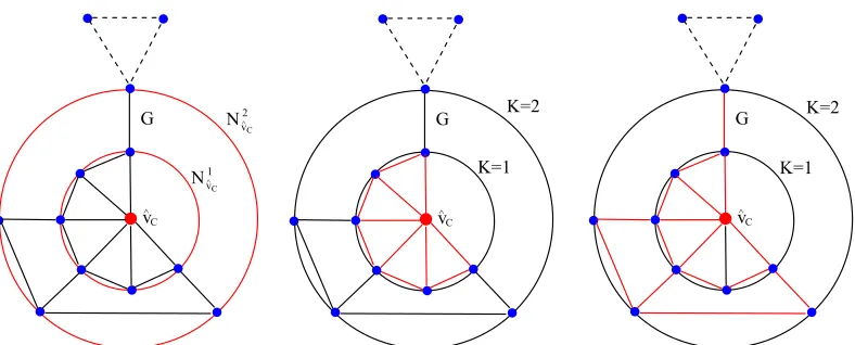
Note that the number of expansion subgraphs is equal to the greatest lengthLof the shortest paths from the centroid vertex to the remaining vertices ofG(V,E). Moreover, theL-layer ex-pansion subgraph isG(V,E) itself. An example of constructing aK-layer expansion subgraph is shown in Fig.1.
Definition 4. (Centroid Depth-based complexity traces)For
a graphG(V,E), let{G1,· · ·,GK,· · ·,GL}be the family ofK
-layer centroid expansion subgraphs rooted at the centroid vertex ofG(V,E). Based on Bai and Hancock (2016), the centroid depth-based complexity trace DB(G) of G(V,E) is computed by measuring the entropies of the subgraphs, i.e.,
Fig. 1. The left-most figure shows the determination ofK-layer centroid expansion subgraphs for a graphG(V,E)which hold|N1 ˆ
vC|= 6and|N
2 ˆ vC|=10
vertices. While the middle and the right-most figure show the corresponding1-layer and2-layer subgraphs regarding the centroid vertexˆvC, and are
depicted by red-colored edges. In this example, the vertices of differentK-layer subgraphs regarding the centroid vertexvˆCare calculated by Eq.(15), and
pairwise vertices possess the same connection information in the original graphG(V,E).
whereH(GK) is the entropy measure of theK-layer expansion
subgraphGK, and it can be either the approximate von
Neuman-n eNeuman-ntropy defiNeuman-ned by Eq.(11) or the ShaNeuman-nNeuman-noNeuman-n eNeuman-ntropy defiNeuman-ned by
Eq.(13). ✷
Based on Bai and Hancock (2016), the centroid depth-based complexity trace has a number of interesting proper-ties. First, it encapsulates the entropy-based information con-tent flow through the family ofK-layer centroid expansion sub-graphs rooted at the centroid vertex, and thus reflects rich in-trinsic depth topology information of a graph. Second, it can be efficiently computed on large graphs. This is because it is computed on a small set of expansion subgraphs rooted at the centroid vertex, and the computational complexity is polynomi-al.
Furthermore, we observe that the centroid depth-based com-plexity trace DB(G)={H(G1),· · ·,H(GK),· · ·,H(GL)}of each
graphG also preserves nest property, i.e., the entropy-based complexity information of each K-layer expansion subgraph encapsulates the information of the 1-layer toK−1-layer expan-sion subgraphs. This follows the fact that the family ofK-layer expansion subgraphs rooted at the centroid vertex ˆvCofG con-structs a nested sequence. Specifically, based on Eq.(17), we observe that the family of expansion subgraphs satisfies
ˆ
vC∈G1· · ·⊆GK⊆· · ·⊆GL⊆G.
In other words, it represents a sequence of subgraphs that grad-ually expand from the centroid vertex to the global graph struc-ture, and eachK-layer expansion subgraph completely encap-sulates the structure information from the lower layer expansion graphs, i.e., the 1-layer toK−1-layer expansion subgraphs. As a result of its nested nature, the centroid depth-based complex-ity trace can be seen as a nested complexcomplex-ity traces that natural-ly reflects both the local and global structure information of a graph.
In a summary, the centroid depth-based complexity trace pro-vides an elegant way of developing novel fast graph kernels that simultaneously consider local and global graph structures.
3. The Local-Global Nested Graph Kernel
In this section, we introduce two novel local-global nested graph kernels, namely the nested aligned kernel and the nest-ed reproducing kernel, that can reflect both the local and global graph characteristics through the centroid depth-based repre-sentations. Specifically, the first nested graph kernel is based on the dynamic time warping measure between the centroid depth-based complexity traces. On the other hand, the second nested graph kernel is based on the basic reproducing kernel between the centroid depth-based complexity traces. We show that both of the kernels can be computed in polynomial time.
3.1. The Nested Graph Kernels
LetGP(VP,EP) andGQ(VQ,EQ) be a pair of graphs, from a graph setG. We commence by computing the centroid depth-based complexity traces ofGPandGQ rooted at their centroid vertices as
DB(GP)={H(GP;1),· · ·,H(GP;K),· · ·,H(GP;Lmax)}
and
DB(GQ)={H(GQ;1),· · ·,H(GQ;K),· · ·,H(GQ;Lmax)},
respectively, whereGP;K andGQ;K are the K-layer expansion subgraphs rooted at the centroid vertices ofGPandGQ,Lmaxis the greatest length of the shortest paths rooted at the centroid vertices over all graphs inG, and the entropy measureH(.) of a
K-layer expansion subgraph can be either the approximate von Neumann entropy defined in Eq.(11) or the Shannon entropy defined in Eq.(13). Note that, forGPandGQ, if their greatest lengths MandNof the shortest paths rooted at their centroid vertices satisfy K ≥ M andK ≥ N, their K-layer expansion subgraphs are their global structures. We consider two alterna-tive ways to define nested graph kernels based on the centroid depth-based representations.
nested aligned graph kernelkNAKbetweenGPandGQas kNAK(GP,GQ)=kGA{DB(GP),DB(GQ)}
=
%
π∈A(Lmax,Lmax)
e−DP,Q(π), (19)
whereπdenotes the warping alignment between DB(GP) and DB(GQ), A(Lmax,Lmax) denotes all possible alignments, and DP,Q(π) is the alignment cost defined in Eq.(3). Note that,
al-though our kernel is based on the global alignment kernelkGA
that is a positive definite kernel, the time series compared by
kNAKare not defined over the same underlying space but on two
different graphs. Thus, we cannot prove that the the proposed kernelkNAKis positive definite. In our future work, we will fur-ther explore the possibility of creating a positive definite kernel by computing the depth-based complexity traces over a com-mon structure obtained by combining the input graphs, e.g., a union graph that preserves the structural information of all graphs.
Assume we have a pair of graphs each havingnvertices and
m edges, computing the nested aligned kernel kNAK requires
time complexity O(mlogn+ L2max). This is because
identi-fying the centroid vertex and computing the centroid depth-based complexity trace of a graph rely on the computation of the shortest path matrix and both of the two processes require time complexityO(mlogn). Furthermore, computing all possi-ble alignments between the depth-based complexity traces has time complexityO(L2
max), whereLmax is the greatest length of
the shortest paths rooted at the centroid vertices of all graphs (note thatLmaxis usually much lower than the vertex numbern
and the edge numberm). As a result, the proposed kernelkNAK
has polynomial time complexityO(mlogn+L2max).
Definition 6. (The Nested Reproducing Kernel)Based on the
basic reproducing kernelK1defined in Section 2.2, we develop a new nested reproducing graph kernelkNRK betweenGP and
GQas
kNRK(GP,GQ)=kNRK{DB(GP),DB(GQ)}
= Lmax %
K=1
K1{H(GP;K),H(GQ;K)}
= 1
2
Lmax %
K=1
e−|H(GP;K)−H(GQ;K)|. (20) The entropy measure H(.) can be either the approximate von Neumann entropy or the Shannon entropy. Moreover, unlike
kNAK, we can guarantee that the proposed nested reproducing
kernelkNRK is positive definite (pd). This is because the
as-sociated basic reproducing kernelK1{HS(GP;K),HS(GQ;K)}
be-tween each pair ofK-layer expansion subgraphs ispd, and the resulting nested reproducing kernelkNRK(GP,GQ) can be seen as the sum of thepdkernelK1betweenLmaxpairs of K-layer
expansion subgraphs.
Assume we have a pair of graphs each havingnvertices and
m edges. Computing the nested reproducing kernelkNRK re-quires time complexityO(mlogn+Lmax). This is because, as we have stated, computing the centroid depth-based complex-ity trace of each graph requires time complexcomplex-ity O(mlogn).
Moreover, computing the reproducing kernel K1 between the
entropies of theLpairs ofK-layer expansion subgraphs requires time complexityO(Lmax). As a result, the proposed kernelkNRK
has polynomial time complexityO(mlogn+Lmax). Compar-ing to the proposed nested aligned kernelkNAK that has time
complexityO(mlogn+L2max), the proposed nested reproducing
kernelkNRKhas more efficient computational complexity. 3.2. Discussions and Related Works
As we have stated in Section 2.4, the required centroid depth-based complexity trace for the proposed nested kernels gauges the entropy-based complexities on theK-layer expansion sub-graphs rooted at the centroid vertex. Since the family of these expansion subgraphs gradually lead the centroid vertex to the global graph structure, the centroid depth-based complexity trace can be seen as a nested complexity trace that naturally re-flects both the local and global structure information of a graph. As a result, either of the proposed graph kernels can be seen as a local-global nested graph kernel that simultaneously cap-tures local and global graph characteristics. Our proposed ker-nels overcome the gap between the local kerker-nels (i.e., kerker-nels based on local substructures of limited sizes proposed by Har-chaoui and Bach (2007); Kriege and Mutzel (2012); Kriege et al. (2016)) and the global kernels (i.e., global kernels based on either the adjacency matrix or the continuous-time quantum walk proposed by Johansson et al. (2014); Xu et al. (2015); Bai and Hancock (2013)). Furthermore, our proposed local-global nested graph kernels are based on a small number of dominant
K-layer expansion subgraphs rooted at the centroid vertex, and thus have more efficient computational complexity than state-of-the-art graph kernels based on a large number of substruc-tures.
the largest layer expansion subgraph of a graph rooted at the centroid vertex is just the global structure of the graph, thus the hybrid reproducing kernel can be seen as the basic reproducing kernel between both the von Neumann and Shannon entropies of the largest layer expansion subgraphs. As a result, the o-riginal hybrid reproducing kernel is just a special case of the proposed nested reproducing kernel and only reflects a part of information of the proposed nested reproducing kernel.
Finally, note that, both the proposed local-global nested graph kernels are also related to the fast Jensen-Shannon sub-graph kernel developed by Bai and Hancock (2016), since they are all based on the similarity measure between the nested cen-troid depth-based complexity traces. However, the fast Jensen-Shannon subgraph kernel is based on the Jensen-Jensen-Shannon di-vergence measure between each pair ofK-layer expansion sub-graphs, and this divergence measure does not encapsulate the alignment information between the probability distributions of the subgraphs. As a result, unlike the proposed nested graph k-ernels, this subgraph kernel cannot reflect precise kernel based similarity measures between the centroid depth-based complex-ity traces of graphs. These above observations indicate the the-oretical advantages of the proposed local-global nested graph kernels.
4. Experimental Evaluations
In this section, we evaluate the performance of the proposed local-global nested graph kernels. We commence the by ex-hibiting the nest property of the centroid depth-based complex-ity traces. Finally, we perform the proposed kernels on graph classification tasks.
4.1. Graph Datasets
We evaluate our kernels on standard graph datasets. These datasets include: MUTAG, PTC, COIL5, Shock, CATH2, Reeb and D&D. Details of these datasets are shown in Table 1.
MUTAG:The MUTAG dataset consists of graphs representing
188 chemical compounds labeled according to whether or not they affect the frequency of genetic mutations in the bacteri-umSalmonella typhimuriumsand aims to predict whether each compound is associated with mutagenicity.
PTC:The PTC (The Predictive Toxicology Challenge) dataset records the carcinogenicity of several hundred chemical com-pounds for male rats (MR), female rats (FR), male mice (MM) and female mice (FM). These graphs are very small, i.e., 20−30 vertices, and sparsem, i.e., 25−40 edges. We select the graphs of male rats (MR) for evaluation. There are 344 test graphs in the MR class.
COIL5: The COIL5 dataset is abstracted from the COIL
im-age database. The COIL database consists of imim-ages of 100 3D objects. In our experiments, we use the images for the first five objects. For each of these objects we employ 72 images captured from different viewpoints. For each image we first ex-tract corner points using the Harris detector, and then establish Delaunay graphs based on the corner points as vertices. Each vertex is used as the seed of a Voronoi region, which expand-s radially with a conexpand-stant expand-speed. The linear colliexpand-sion frontexpand-s of
the regions delineate the image plane into polygons, and the Delaunay graph is the region adjacency graph for the Voronoi polygons.
Shock: The Shock dataset consists of graphs from the Shock
2D shape database. Each graph is a skeletal-based representa-tion of the differential structure of the boundary of a 2D shape. There are 150 graphs divided into 10 classes.
CATH2: The CATH2 dataset is harder to classify, since the
proteins in the same topology class are structurally similar. The protein graphs are 10 times larger in size than chemical com-pounds, with 200 . 300 vertices. There is 190 testing graphs in the dataset.
Reeb: The SHREC 3D Shape database consists of 15 classes
and 20 individuals per class, that is 300 shapes Biasotti et al. (2003). This is a standard benchmark in 3D shape recogni-tion. From the SHREC 3D Shape database, we establish a Reeb graph datasets through a mapping functions. This functions is ERG barycenter that computes the distance from the center of mass/barycenter. Details of the three mapping function can be found in Biasotti et al. (2003). The number of maximum, mini-mum and average vertices for the three datasets are 220, 41 and 95.42 respectively.
D&D:The D&D dataset contains 1178 protein structures. Each protein is represented by a graph, in which the vertices are amino acids and two vertices are connected by an edge if they are less than 6 Angstroms apart. The prediction task is to clas-sify the protein structures into enzymes and non-enzymes. The maximum, minimum and average number of vertices are 5748, 30 and 284.32 respectively.
4.2. Evaluations of the Nested Centroid Depth-based Complex-ity Traces
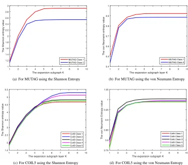
In this subsection, we investigate the nest property of the cen-troid depth-based complexity trace. In the experiment, we u-tilize the testing graphs in the MUTAG and COIL5 datasets. Based on Table 1, the MUTAG and COIL5 datasets represent the testing graphs with low and high average degrees (i.e., 1.10 versus 2.89) respectively. For each testing graph, we commence by identifying the centroid vertex and establish a family ofK -layer expansion subgraphs rooted at the vertex. Moreover, we compute the approximate von Neumann entropy or the Shan-non entropy associated with the steady state random walk on each of the expansion subgraphs, as the centroid depth-based complexity trace of the graph. For each dataset, we compute the mean centroid depth-based complexity trace of the graphs from the same class. We draw the mean complexity trace and the experimental results are shown in Fig. 2.
The subfigures of Fig. 2 exhibit the mean centroid depth-based complexity trace, and each colorized line represents the mean complexity trace of the graphs belonging to the same class in a dataset. Here, the subfigures (a) and (b) are for the MUTAG dataset using the Shannon and von Neumann entropies respectively. The subfigures (c) and (d) are for the COIL5 dataset using the Shannon and von Neumann entropies respec-tively. For each subfigure, the x-axis shows the order of the
Table 1. Information on the selected graph based bioninformatics datasets
Datasets MUTAG PTC COIL Shock CATH2 Reeb D&D
Max # vertices 28 109 241 33 568 220 5748
Min # vertices 10 2 72 4 143 41 30
Mean # vertices 17.93 25.60 144.90 109.63 308.03 95.42 284.3
Max # edges 33 108 702 32 2220 219 14267
Min # edges 10 1 206 3 556 40 63
Mean # edges 19.79 25.96 419 12.16 1254.80 94.59 715.65
# graphs 188 344 360 150 190 300 1178
# classes 2 2 5 5 2 15 2
Mean#edges/Mean#vertices 1.10 1.00 2.89 0.92 4.07 0.99 2.52
The expansion subgraph K
1 2 3 4 5 6 7 8 9 10
T
h
e
Sh
a
n
n
o
n
e
n
tro
p
y
va
lu
e
1 1.2 1.4 1.6 1.8 2 2.2 2.4 2.6 2.8 3
MUTAG Class 1 MUTAG Class 2
(a) For MUTAG using the Shannon Entropy
The expansion subgraph layer K
1 2 3 4 5 6 7 8 9 10
T
h
e
vo
n
N
e
u
ma
n
n
e
n
tro
p
y
va
lu
e
0.4 0.5 0.6 0.7 0.8 0.9 1
MUTAG Class 1 MUTAG Class 2
(b) For MUTAG using the von Neumann Entropy
The expansion subgraph layer K
1 2 3 4 5 6 7 8 9 10
T
h
e
Sh
a
n
n
o
n
e
n
tro
p
y
va
lu
e
1.5 2 2.5 3 3.5 4 4.5 5 5.5
Coil5 Class 1 Coil5 Class 2 Coil5 Class 3 Coil5 Class 4 Coil5 Class 5
(c) For COIL5 using the Shannon Entropy
The expansion subgraph K
1 2 3 4 5 6 7 8 9 10
T
h
e
vo
n
N
e
u
ma
n
n
En
tro
p
y
va
lu
e
0.75 0.8 0.85 0.9 0.95 1 1.05
Coil5 Class 1 Coil5 Class 2 Coil5 Class 3 Coil5 Class 4 Coil5 Class 5
(d) For COIL5 using the von Neumann Entropy
[image:9.595.108.486.361.693.2]From Fig. 2, we observe that the mean entropy values tend to be larger with the increasing layer sizeK of the expansion subgraphs. This is because the family of the K-layer expan-sion subgraphs rooted at the centroid vertex tend to gradual-ly lead the local centroid vertex to the global graph structure, and each K-layer expansion subgraph encapsulates the struc-ture information of the 1-layer to K−1-layer expansion sub-graphs. As a result, Fig. 2 demonstrates the nest property of the centroid depth-based complexity traces, i.e., the entropy-based complexity information of eachK-layer expansion sub-graph encapsulates the information of the 1-layer toK−1-layer expansion subgraphs. Furthermore, it is clear that the mean centroid depth-based complexity traces of graphs from differ-ent classes are dissimilar. This indicates that the cdiffer-entroid depth-based complexity traces have good ability to distinguish graphs from different classes. Finally, we observe that, for the COIL5 dataset the complexity traces using the Shannon entropy can better distinguish the graphs from different classes than that us-ing the von Neumann entropy. On the other hand, for the MU-TAG dataset the complexity traces using either the Shannon en-tropy or the von Neumann enen-tropy can both well distinguish the graphs from different classes. This is because the average vertex degree of the COIL5 dataset is obviously larger than that of the MUTAG dataset. As we have stated in Section 2.3, the von Neumann entropy is sensitive to graphs having low vertex degrees, while the Shannon entropy is suited to characterizing graphs with high vertex degrees. As a result, the centroid depth-based complexity trace using the Shannon entropy is more suit-able to the dataset having graphs with high vertex degrees than that using the von Neumann entropy.
4.3. Experiments on Graph Classification
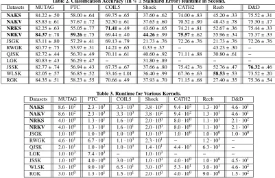
In this subsection, we investigate the performance of the pro-posed local-global nested graph kernels. Specifically, we evalu-ate the classification accuracies of the nested aligned kernel as-sociated with the von Neumann entropy (NAKV) and the Shan-non entropy (NAKS), and those of the nested reproducing ker-nel associated with the von Neumann entropy (NRKV) and the Shannon entropy (NRKS) on a number of graph classification tasks. Furthermore, we also compare our proposed nested graph kernels with seven state-of-the-art graph kernels, including 1) the Jensen-Shannon graph kernel (JSGK) Bai and Hancock (2013), 2) the random walk graph kernel (RWGK) Kashima et al. (2003), 3) the unaligned quantum Jensen-Shannon graph kernel (QJSK) Bai et al. (2015a), 4) the Lov´asz graph ker-nel (LGK) Johansson et al. (2014), 5) the fast Jensen-Shannon subgraph kernel Bai and Hancock (2016), 6) the Weisfeiler-Lehman subtree kernel (WLSK) Shervashidze et al. (2010), and 7) the reproducing graph kernel (RGK) Xu et al. (2018). For the WLSK kernel, we set the largest iteration of the required vertex label strengthening methods as 10, and we use the vertex degree as the original vertex label.
We compute the kernel matrix associated with each kernel on each dataset. We perform 10-fold cross-validation using a C-Support Vector Machine (C-SVM) to compute the classifica-tion accuracies, using LIBSVM software library Chang and Lin (2011). We use nine samples for training and one for testing.
The parameters of the C-SVMs are optimized on each training set using cross-validation. We report the average classification accuracy and the runtime for each kernel in Table 2 and Ta-ble 3. The runtime is measured under Matlab R2015a running on a 2.5GHz Intel 2-Core processor (i.e., i5-3210m).
In terms of classification accuracies on different graph datasets, Table 2 indicates that the proposed local-global nest-ed graph kernels outperform or are competitive to most alter-native graph kernels. Especially, the proposed NRKV kernel significantly outperforms all alternative graph kernels on most datasets. Only the classification accuracy of the WLSK kernel on the Reeb dataset and that of the JSSK kernel on the D&D dataset are a little higher than the proposed NRKV kernel, but our NRKV kernel is still competitive. The reason of the effec-tiveness is that, as we have stated, our proposed nested graph kernels can simultaneously capture the local and global graph characteristics. By contrast, the local graph kernels RWGK and WLSK can only reflect local characteristics of graphs based on substructures, while the global graph kernels JSGK, QJSK, L-GK and RL-GK can only capture global characteristics based on global matrix representations of graphs (e.g., the Laplacian or the adjacency matrix). On the other hand, similar to the pro-posed nested graph kernel the JSSK can also reflect both the lo-cal and global graph characteristics, relying on the depth-based representation. Unfortunately, as we have stated in Section 3.2, the required Jensen-Shannon divergence measure of the JSSK kernel does not establish the alignment information between the probability distributions of pairwise graphs. As a result, the JSSK kernel cannot reflect the precise kernel based similarity information between graphs.
Overall, the classification accuracies of the nested reproduc-ing kernels (i.e., the NRKS and NRKV kernels) are significant-ly better than those of the nested aligned kernels (i.e., the NAKS and NAKV kernels), especially on the PTC, Shock and Reeb datasets. Through Table 1, we observe that the average vertex degrees of the PTC, Shock and Reeb datasets are smaller than 1. On the other hand, the average vertex degrees of the COIL5, CATH2 and D&D datasets are significantly higher, and the clas-sification accuracies of the nested reproducing kernels and the nested aligned kernels on these datasets are competitive. This observation indicates that the nested aligned kernel is not suit-able for graph datasets have low average vertex degrees, and the nested reproducing kernels has better applicability on any dataset.
Furthermore, we observe that either of the proposed nested kernels associated with the von Neumann entropy significant-ly outperforms that associated with the von Shannon entropy on the MUTAG, PTC, Shock and Reeb datasets. This is be-cause the graphs from these datasets have lower average vertex degrees than the remaining datasets. As we have stated in Sec-tion 2.3, the von Neumann entropy is suitable to graphs having low vertex degrees. This suggests that for graph datasets having low vertex degrees the proposed nested kernels associated with the von Neumann entropy are more preferable.
com-Table 2. Classification Accuracy (In%±Standard Error) Runtime in Second.
Datasets MUTAG PTC COIL5 Shock CATH2 Reeb D&D
NAKS 84.22±.50 58.00±.64 69.75±.65 37.60±.62 74.00±.83 45.20±.33 75.52±.31
NAKV 83.83±.61 57.67±.72 52.50±.61 37.65±.60 70.52±.90 48.43±.78 75.30±.17
NRKS 82.25±.63 55.05±.77 71.41±.49 43.60±.65 74.21±.81 52.67±.36 75.44±.33
NRKV 84.37±.78 59.26±.75 69.44±.40 44.26±.99 75.57±.62 55.96±.34 75.37±.33
JSGK 83.11±.80 57.29±.41 69.13±.79 21.73±.76 72.26±.76 21.73±.76 72.26±.76
RWGK 80.77±.75 53.97±.31 14.21±.65 0.33±.37 − 43.23±.30 −
QJSK 82.72±.44 56.70±.49 70.11±.61 40.60±.92 71.11±.88 30.80±.61 −
LGK 80.83±.43 56.29±.47 − 31.80±.89 − − −
JSSK 82.77±.74 56.94±.43 67.75±.67 37.66±.80 75.42±.76 52.76±.47 76.32±.46
WLSK 82.05±.57 56.85±.52 33.16±1.01 36.40±.99 67.36±.63 58.53±.53 73.52±.20
RGK 84.35±.51 58.23±.55 70.66±.49 37.93±.70 71.15±.68 27.40±.35 75.36±.54
Table 3. Runtime for Various Kernels.
Datasets MUTAG PTC COIL5 Shock CATH2 Reeb D&D
NAKS 8.6·102 2.3·103 3.3·103 3.8·102 9.4·102 1.3·101 4.6·101
NAKV 8.6·102 2.3·103 3.3·103 3.8·102 9.4·102 1.3·101 4.6·101
NRKS 4.0·100 1.3·101 1.6·101 2.0·100 8.0·100 1.1·101 2.1·102
NRKV 4.0·100 1.3·101 1.6·101 2.0·100 8.0·100 1.1·101 2.1·102
JSGK 1.0·100 1.0·100 1.0·100 1.0·100 1.0·100 1.0·100 1.0·100
RWGK 4.6·101 6.7·101 1.1·103 2.3·101 − 1.2·103 −
QJSK 2.0·101 1.0·102 1.0·103 1.4·101 4.4·103 6.3·103 −
LGK 1.0·103 7.4·103 − 1.0·103 − − −
JSSK 1.0·100 4.0·100 3.0·100 1.0·100 4.0·100 1.0·100 4.5·101
WLSK 3.0·100 9.0·101 6.5·101 3.0·100 5.3·101 3.0·101 4.6·102
RGK 3.0·100 1.3·101 1.5·101 2.0·100 4.0·100 9.0·100 1.5·102
plete the computation of the kernel matrices. By contrast, some alternative graph kernels (e.g., the LGK and RWGK kernels) fail to complete the computation in a reasonable time. On the other hand, the proposed nested reproducing kernels have com-petitive computational efficiency to the fast alternative JSGK and JSSK kernels.
5. Conclusion
In this paper, we have proposed two novel local-global nested graph kernels, namely the nested aligned kernel and the nested reproducing kernel. Both of the nested kernels are based on the centroid depth-based complexity traces, that gauge the nested depth complexity trace through a family of K-layer expansion subgraphs rooted at the centroid vertex. Unlike most existing state-of-the-art graph kernels that only probe local or global graph characteristics, the proposed nested kernels simultane-ously consider the local and global graph characteristics and thus reflect the presence of richer structural patterns. The ex-periments have demonstrated the effectiveness and efficiency of the proposed nested kernels.
Our future work is to extend the proposed kernel to attributed graphs that encapsulate vertex and edge labels. Moreover, we would also like to further develop novel graph kernels through the dynamic time warping framework associated with other types of (hyper)graph characteristic sequences, e.g., the cycle numbers identified by the Ihara zeta function, the time-varying entropies computed from the continuous-time or discrete-time quantum walk Bai et al. (2015a, 2017). Finally, we are also interested in developing novel graph kernels for time-varying financial market networks Ye et al. (2015), using the dynamic time warping framework.
Acknowledgments
This work is supported by the National Natural Science Foundation of China (Grant no. 61503422, 61602535, 61773415, 61370123 and 61772057), the Open Projects Pro-gram of National Laboratory of Pattern Recognition, the pro-gram for innovation research in Central University of Finance and Economics, and the Beijing Natural Science Foundation project (no. 4162037).
References
Alvarez, M.A., Qi, X., Yan, C., 2011. A shortest-path graph kernel for estimat-ing gene product semantic similarity. J. Biomedical Semantics 2, 3. Aronszajn, N., 1950. Theory of reproducing kernels. Transactions of the
Amer-ican mathematical society .
Bach, F.R., 2008. Graph kernels between point clouds, in: Proceedings of ICML, pp. 25–32.
Bai, L., Hancock, E.R., 2013. Graph kernels from the jensen-shannon diver-gence. Journal of mathematical imaging and vision 47, 60–69.
Bai, L., Hancock, E.R., 2014. Depth-based complexity traces of graphs. Pattern Recognition 47, 1172–1186.
Bai, L., Hancock, E.R., 2016. Fast depth-based subgraph kernels for unattribut-ed graphs. Pattern Recognition 50, 233–245.
Bai, L., Rossi, L., Cui, L., Zhang, Z., Ren, P., Bai, X., Hancock, E.R., 2017. Quantum kernels for unattributed graphs using discrete-time quantum walks. Pattern Recognition Letters 87, 96–103.
Bai, L., Rossi, L., Torsello, A., Hancock, E.R., 2015a. A quantum jensen-shannon graph kernel for unattributed graphs. Pattern Recognition 48, 344– 355.
Bai, L., Rossi, L., Zhang, Z., Hancock, E.R., 2015b. An aligned subtree kernel for weighted graphs, in: Proceedings of ICML, pp. 30–39.
Biasotti, S., Marini, S., Mortara, M., Patan`e, G., Spagnuolo, M., Falcidieno, B., 2003. 3d shape matching through topological structures, in: Proceedings of DGCI, pp. 194–203.
Chang, C.C., Lin, C.J., 2011. Libsvm: a library for support vector machines. ACM Transactions on Intelligent Systems and Technology 2, 27. Conte, D., Ramel, J., Sidere, N., Luqman, M.M., Ga¨uz`ere, B., Gibert, J., Brun,
[image:11.595.100.501.82.342.2]Costa, F., De Grave, K., 2010. Fast neighborhood subgraph pairwise distance kernel, in: Proceedings ICML, pp. 255–262.
Cuturi, M., 2011. Fast global alignment kernels, in: Proceedings of ICML, pp. 929–936.
Cuturi, M., Vert, J., Birkenes, Ø., Matsui, T., 2007. A kernel for time series based on global alignments, in: Proceedings of ICASSP, pp. 413–416. Farhi, E., Gutmann, S., 1998. Quantum computation and decision trees.
Phys-ical Review A 58, 915.
Haasdonk, B., Bahlmann, C., 2004. Learning with distance substitution kernels, in: Proceedings of DAGM, pp. 220–227.
Han, L., Escolano, F., Hancock, E.R., Wilson, R.C., 2012. Graph characteri-zations from von neumann entropy. Pattern Recognition Letters 33, 1958– 1967.
Harchaoui, Z., Bach, F., 2007. Image classification with segmentation graph kernels, in: Proceedings of CVPR, pp. 1–8.
Johansson, F.D., Jethava, V., Dubhashi, D.P., Bhattacharyya, C., 2014. Global graph kernels using geometric embeddings, in: Proceedings of ICML, pp. 694–702.
Kashima, H., Tsuda, K., Inokuchi, A., 2003. Marginalized kernels between labeled graphs, in: Proceedings of ICML, pp. 321–328.
Kriege, N., Mutzel, P., 2012. Subgraph matching kernels for attributed graphs, in: Proceedings of ICML.
Kriege, N.M., Giscard, P., Wilson, R.C., 2016. On valid optimal assignment kernels and applications to graph classification, in: Proceedings of NIPS, pp. 1615–1623.
Ren, P., Aleksi´c, T., Wilson, R.C., Hancock, E.R., 2011. A polynomial charac-terization of hypergraphs using the ihara zeta function. Pattern Recognition 44, 1941–1957.
Riesen, K., Bunke, H., 2010. Graph classification and clustering based on vec-tor space embedding. World Scientific Publishing Co., Inc.
Rossi, L., Torsello, A., Hancock, E.R., 2015. Measuring graph similarity
through continuous-time quantum walks and the quantum jensen-shannon divergence. Physical Review E 91, 022815.
Shervashidze, N., Schweitzer, P., van Leeuwen, E.J., Mehlhorn, K., Borgwardt, K.M., 2010. Weisfeiler-lehman graph kernels. Journal of Machine Learning Research 1, 1–48.
Urry, M., Sollich, P., 2013. Random walk kernels and learning curves for gaus-sian process regression on random graphs. Journal of Machine Learning Research 14, 1801–1835.
Wang, L., Sahbi, H., 2013. Directed acyclic graph kernels for action recogni-tion, in: Proceedings of ICCV, pp. 3168–3175.
Xu, L., Jiang, X., Bai, L., Xiao, J., Luo, B., 2018. A hybrid reproducing graph kernel based on information entropy. Pattern Recognition 73, 89–98. Xu, L., Niu, X., Xie, J., Abel, A., Luo, B., 2015. A local–global mixed kernel
with reproducing property. Neurocomputing 168, 190–199.
Xu, L., Niu, X.C.X., Zhang, C., Luo, B., 2017. A multiple attributes convo-lution kernel with reproducing property. Pattern Analysis and Applications 20, 485C494.