Squint mode GEO SAR imaging using bulk range walk correction on received signals

This is a repository copy of

Squint mode GEO SAR imaging using bulk range walk

correction on received signals

.

White Rose Research Online URL for this paper:

http://eprints.whiterose.ac.uk/141456/

Version: Published Version

Article:

Geng, J., Yu, Z., Li, C. et al. (1 more author) (2019) Squint mode GEO SAR imaging using

bulk range walk correction on received signals. Remote Sensing, 11 (1). 17. ISSN

2072-4292

https://doi.org/10.3390/rs11010017

[email protected] https://eprints.whiterose.ac.uk/

Reuse

This article is distributed under the terms of the Creative Commons Attribution (CC BY) licence. This licence allows you to distribute, remix, tweak, and build upon the work, even commercially, as long as you credit the authors for the original work. More information and the full terms of the licence here:

https://creativecommons.org/licenses/

Takedown

If you consider content in White Rose Research Online to be in breach of UK law, please notify us by

remote sensing

Article

Squint Mode GEO SAR Imaging Using Bulk Range

Walk Correction on Received Signals

Jiwen Geng1, Ze Yu1,*, Chunsheng Li1and Wei Liu2

1 _{School of Electronic and Information Engineering, Beihang University, Beijing 100191, China;}

[email protected] (J.G.); [email protected] (C.L.)

2 _{Department of Electronic & Electrical Engineering, University of Sheffield, Sheffield S1 4ET, UK;}

[email protected]

* Correspondence: [email protected]; Tel.: +86-185-1920-7286

Received: 11 September 2018; Accepted: 19 December 2018; Published: 21 December 2018

Abstract: Geosynchronous synthetic aperture radar (GEO SAR) has the potential for conducting long-term observation of target zones, which is essential for remote sensing applications such as disaster monitoring and vegetation measurements. The squint imaging mode is crucial for long-term observation using GEO SAR. However, this type of SAR imaging is problematic because the squint mode introduces a nonzero range cell walk, which increases the prevalence of invalid data in echoes and intensifies the coupling between the azimuth and range. Therefore, this paper proposes a novel squint mode GEO SAR imaging method based on the correction of the bulk range walk of received signals. Adjusting the starting time of the receiving window significantly reduces the redundancy in echoes. Then, first-order filtering, range cell migration correction, range compression, partial dechirp, and azimuth compression are used to obtain the imaging result. Simulation results for the GEO SAR imaging of Wenchuan County in China demonstrate that the proposed algorithm can achieve a resolution of 5 m within a 30×30 km swath over 48% of the orbital period.

Keywords:geosynchronous synthetic aperture radar; squint mode imaging; range walk correction

1. Introduction

Geosynchronous synthetic aperture radar (GEO SAR) operates on an inclined orbit at a speed of nearly 3.075 km/s and at a height of approximately 35,786 km [1,2]. Compared with low earth orbit (LEO) SAR, GEO SAR moves more slowly and has a wider field of view that is nearly one-third of the earth’s surface [3]. These features enable GEO SAR to observe target zones for a much longer period than LEO SAR, which is beneficial for conducting disaster monitoring [4]. Figure1illustrates an observation mode suitable for long-term observation via GEO SAR. This mode is composed of several strip-map observations acquired with different squint angles, and the target zone is imaged according to the overlapping area of the strip-map data received. Here, not only broadside SAR imaging, but also squint mode SAR imaging, must be used to process echoes acquired by this observation mode. The present study focuses on squint mode strip-map GEO SAR imaging.

Remote Sens.Remote Sens2019,11, 17x FOR PEER REVIEW of2 of 26

A B C D

Target Zone Nadir Trajectory

Stripmap A Stripmap B Stripmap C Stripmap D

Figure Illustration of a geosynchronous synthetic aperture radar GEO SAR observation mode The red point is the center of the target zone The blue line on the map represents the nadir trajectory of the GEO SAR platform The trajectory includes four segments A B C and D denoted by different colors that correspond to separate strip map observations A constant squint angle is adopted in each segment which varies from segment to segment to ensure that the beam center coincides exactly with the red point when the platform resides at the center of each segment Because the orbit of the GEO SAR platform is extremely high the overlapping area of the four strip map observations is sufficiently large to fully image the target zone

Slant Range History of Squint Mode GEO SAR

Figure illustrates the observation geometry between the strip map GEO SAR imaging and a target zone as the GEO SAR platform moves along its orbit At azimuth timetref the beam center points to the reference targetPref which is usually the center of the target zone and the slant range between the beam center andPrefis denoted byRref At the azimuth timetc the beam center points to

Pc and the corresponding slant distance isRc The slant range history of GEO SAR imaging can be analyzed according to Figure as follows

X

Y Z

ref

t tc

ref

R

c

R

O

c

t



ref

R Rc

R



ref

P

c

P

Figure Observation geometry between strip map GEO SAR imaging and a target zone as the GEO SAR platform moves along its orbit The target zone area enclosed by the blue circle in the diagram Figure 1. Illustration of a geosynchronous synthetic aperture radar (GEO SAR) observation mode. The red point is the center of the target zone. The blue line on the map represents the nadir trajectory of the GEO SAR platform. The trajectory includes four segments A, B, C, and D denoted by different colors that correspond to separate strip-map observations. A constant squint angle is adopted in each segment, which varies from segment to segment to ensure that the beam center coincides exactly with the red point when the platform resides at the center of each segment. Because the orbit of the GEO SAR platform is extremely high, the overlapping area of the four strip-map observations is sufficiently large to fully image the target zone.

The relative trajectories between GEO SAR platforms and targets are curved, which varies the range histories spatially in both the azimuth and range directions [5]. A number of GEO SAR imaging algorithms have been developed to correct this two-dimensional (2D) spatial variance. For example, the time-domain back projection (BP) algorithm has been developed for image focusing [6]. However, this algorithm suffers from its tremendous computational burden, even though the fast BP algorithm reduces the computational burden toO(N5/2_{) [7]. In contrast, the computational} complexity of frequency-domain algorithms is much lower, and numerous algorithms that operate in this domain have been developed. The classic frequency-domain SAR imaging algorithms include the omega-K methods presented by Claudio Prati and Fabio Rocca [8], the methods based on the chirp scaling [9], and the frequency domain algorithms proposed by Franceschetti et al. [10]. As aforementioned, the severe spatial variance makes these classical algorithms fail in GEO SAR. However, inspired by these methods, some scholars developed algorithms for GEO SAR. Bao et al. [11] modified the chirp scaling (CS) algorithm based on a fourth-order polynomial model, and achieved an 8-m resolution within a 40×40 km swath. Hu et al. [12] improved the conventional nonlinear CS algorithm by accounting for a linear spatial variance in the range direction in the polynomial model. Tao et al. [13] developed the nonlinear azimuth CS algorithm by introducing spatially variant components in the classic hyperbolic model. Sun et al. [14] considered spatial variation in both the range and azimuth directions in a fifth-order polynomial model, and a 5-m resolution within an 82×95 km swath was achieved using range cell migration (RCM) equalization and sub-band synthesis technologies. To avoid the requirement for conducting sub-band synthesis, Chen et al. [15] combined singular value decomposition and azimuth nonlinear scaling, and obtained a 20-m resolution within a 150×130 km swath. Yu et al. [16] proposed a time-frequency scaling algorithm to correct linear and quadratic variances in the azimuth direction and obtained well-focused results. Ding et al. [17] modified the quadratic term in the azimuth direction and obtained a 20-m resolution within a 400×200 km swath under conditions where the Doppler rate was zero or approximately zero.

Remote Sens.2019,11, 17 3 of 26

between the azimuth and the range. As a result, squint mode SAR imaging is considerably more complicated than broadside imaging. Therefore, correcting the range walk is the key to developing high-resolution squint mode GEO SAR imaging. Whereas past efforts have addressed this issue using range migration removal and 2D nonlinear CS [18], the researchers assumed that the range walk was spatially invariant over the entire swath, which restricted the performance of the developed algorithm. Therefore, we propose a novel squint mode GEO SAR imaging method based on the correction of the bulk range walk of echoes. The key component of the method is to exploit the characteristics of the low pulse repetition frequency (PRF) employed in GEO SAR, and accordingly adjust the starting time of the receiving window. Then, first-order filtering, RCM correction (RCMC), range compression, partial dechirp, and azimuth compression are used to obtain the imaging result. Although the bulk range walk can be corrected in the signal processing stage, the proposed method conducts the correction while receiving the echoes (i.e., during receiving), which significantly reduces the echoes redundancy and improve the efficiency of on-board storage.

The remainder of this paper is structured as follows. Section2analyzes the range walk of squint mode GEO SAR based on a slant range model, and illustrates the advantages of conducting range walk removal upon receiving. Section3discusses the feasibility of conducting range walk removal on receiving by comparing the Doppler bandwidths of GEO SAR and LEO SAR, and presents the proposed approach for adjusting the starting time of the receive window. An imaging algorithm based on echoes with the bulk range walk corrected is then proposed in Section4. Simulation results for the squint mode GEO SAR imaging of Wenchuan County in China are presented and analyzed in Section5, and the results are discussed in Section6. Finally, Section7concludes the paper.

2. Slant Range History of Squint Mode GEO SAR

Figure2illustrates the observation geometry between the strip-map GEO SAR imaging and a target zone as the GEO SAR platform moves along its orbit. At azimuth timetref, the beam center points to the reference targetPref, which is usually the center of the target zone, and the slant range between the beam center andPrefis denoted byRref. At the azimuth timetc, the beam center points to

Pc, and the corresponding slant distance isRc. The slant range history of GEO SAR imaging can be analyzed according to Figure2as follows.

Remote Sens x FOR PEER REVIEW of

A B C D

Target Zone Nadir Trajectory

Stripmap A Stripmap B Stripmap C Stripmap D

Figure Illustration of a geosynchronous synthetic aperture radar GEO SAR observation mode The red point is the center of the target zone The blue line on the map represents the nadir trajectory of the GEO SAR platform The trajectory includes four segments A B C and D denoted by different colors that correspond to separate strip map observations A constant squint angle is adopted in each segment which varies from segment to segment to ensure that the beam center coincides exactly with the red point when the platform resides at the center of each segment Because the orbit of the GEO SAR platform is extremely high the overlapping area of the four strip map observations is sufficiently large to fully image the target zone

Slant Range History of Squint Mode GEO SAR

Figure illustrates the observation geometry between the strip map GEO SAR imaging and a target zone as the GEO SAR platform moves along its orbit At azimuth timetref the beam center points to the reference targetPref which is usually the center of the target zone and the slant range between the beam center andPrefis denoted byRref At the azimuth timetc the beam center points to

Pc and the corresponding slant distance isRc The slant range history of GEO SAR imaging can be analyzed according to Figure as follows

X

Y Z

ref

t tc

ref

R

c

R

O _tc

ref

R Rc

R



ref

P

c

P

Figure Observation geometry between strip map GEO SAR imaging and a target zone as the GEO SAR platform moves along its orbit The target zone area enclosed by the blue circle in the diagram Figure 2.Observation geometry between strip-map GEO SAR imaging and a target zone as the GEO SAR platform moves along its orbit. The target zone area enclosed by the blue circle in the diagram on the left side is enlarged in the diagram on the right side. Attrefandtc, the beam center points to targets

PrefandPc, respectively, wherePrefis the reference target, which is also the center of the target zone.

Attref, the slant range between the beam center andPrefisRref. Attc, the slant range between the beam

Remote Sens.2019,11, 17 4 of 26

Ignoring the antenna weighting, the GEO SAR echo fromPccan be expressed as:

Secho(t,τ) =σ·rect

_t −tc

Ts

·rect

τ−2R(t)/c Tp

·exp

"

jπKr

τ−2R(t)

c

2# ·exp

−j4π

λ R(t)

, (1)

wheretandτdenote the slow time in the azimuth direction and the fast time in the range direction, respectively; σis the radar cross-section of Pc;rect(·) is the rectangle function; Ts is the synthetic aperture time;R(t) represents the slant range history between the beam center andPc;cis the speed of light;Tpis the pulse width of the transmitted chirp signal;Kris the frequency modulation rate; andλis the wavelength of the beam. As previously reported [16],R(t) can be described by a polynomial expression of orderN, as follows:

R(t)≈

N

∑

rn

n!(t−tc) n

, (2)

wherern is thenth polynomial coefficient that can be obtained by fitting based on ephemeris data and geographic information specific to the target zone. A value ofN= 5 has been demonstrated to be sufficiently large for GEO SAR imaging [16], and that value is assumed hereafter. However, becauseR(t) varies for different target zones at different locations, the coefficientsrnare spatially variant, and can be expressed as functions of∆_{R=Rc−Rre f and}∆_{t=tc−tre f, as follows:}

        

       

r0=r0,re f +∆R

r1=r1,re f +k1,1,r·∆R+k1,1,a|∆R·∆t

r2=r2,re f +k2,1,r·∆R+k2,2,r·∆R2+k2,1,a|∆R·∆t+k2,2,a|∆R·∆t2

r3=r3,re f +k3,1,r·∆R+k3,1,a|∆R·∆t+k3,2,a|∆R·∆t2

r4=r4,re f +k4,1,r·∆R+k4,1,a|∆R·∆t

r5=r5,re f

(3)

where the auxiliary coefficientsrn,ref,kn,m,r, andkn,m,a|∆R, wherekn,m,a|∆Rdenotes the spatially variant coefficientkn,m,rat∆R, can be calculated as presented previously in Yu et al. [16].

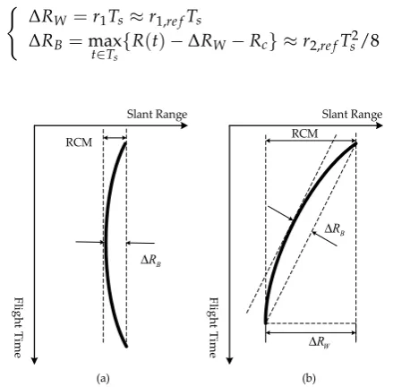
As Figure3shows, echoes usually contain range walk∆_{RWand range curvature}∆_{RB. According to} Equation (2), the first-order coefficientr1mainly causes the range walk. Therefore, the range walk and the range curvature are given as follows:

( _∆

RW =r1Ts≈r1,re fTs ∆_RB=max

t∈Ts

{R(t)−∆_{RW−Rc} ≈r2,re fT}2

s/8 (4)

 

   

  _{   }  

 

  _{   }  

  _ _{    }  



          

W

R ∆

B

R ∆

Slant Range

F

lig

h

t T

im

e

RCM Slant Range

F

lig

h

t T

im

e

RCM

B

R ∆

(a) (b)

  

Remote Sens.2019,11, 17 5 of 26

In frequency domain squint mode GEO SAR imaging, both∆_RWand∆_{RBshould be corrected to} make the migration curve limited in one single range bin.

To evaluate the proportion of∆RWrequiring correction, we define a ratioχWas:

χW=

∆_RW ∆RW+∆RB ≈

8r1,re f

8r1,re f +r2,re fTs. (5)

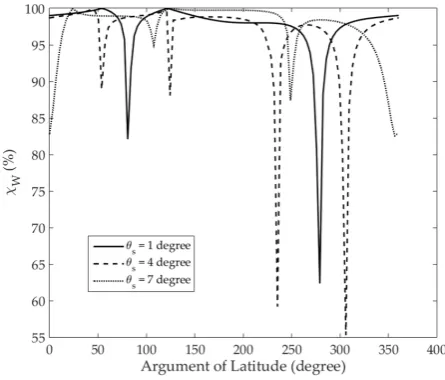
Figure4illustrates the value ofχWobtained for different squint anglesθs, where the GEO SAR platform operates on an orbit with an inclination angle of 60◦. Here, we note that χW generally increases with increasingθs.χWis greater than 90% for the most of the orbital period. This indicates that∆_{RWaccounts for the vast majority of the correction required. We note that for a swath of width} ∆_{W, the volume of recorded echo data can be given as:}

Vecho≈

2

c

∆W·sinθinc+

cTp

2 +max{∆RB,∆RW}

·Fs·Na, (6)

whereθincis the incidence angle corresponding to the center of the target zone,Fsis the range sampling rate, and Na is the azimuth sampling rate. From Equation (5), the ratio ∆RW/∆RB is given by χW/(1−χW), which means∆RW is much higher than 9 times of∆RB. Equation (6) indicates that

Vechois significantly reduced if∆RWis corrected on receiving rather than storing the data for later image processing. Consequently, the efficiency of on-board GEO SAR data storage increases.

 

 

 

 

,

Figure 4. Values of ratioχW, defined in Equation (5), obtained with different squint anglesθs,

which include 1, 4, and 7 degrees. Because of the high orbital height, the maximum value ofθs

is approximately 7◦for GEO SAR.

3. Bulk Range Walk Correction on Receive

Compared with LEO SAR, the Doppler band of GEO SAR is much narrower. This feature makes it feasible to conduct bulk range walk correction by adjusting the starting time of the receiving window. The specific features of GEO SAR and the proposed adjustment principle are presented in the following discussion.

3.1. Doppler Bandwidth of GEO SAR

Remote Sens.2019,11, 17 6 of 26

As illustrated in Figure5, a GEO SAR platform moves fromS1toS2while observingPc.S0is the midpoint of the arcS1ˆS2. The corresponding Doppler bandwidth is:

Ba=|fd2−fd1|, (7)

wherefd1andfd2are the instantaneous Doppler frequencies atS1andS2, respectively, which are given as follows:

fd1= (2/λ)·

→

Vst1·

_→

Rt−

→

Rs1

/|→Rt−

→

Rs1| (7a)

fd2= (2/λ)·

→

Vst2·

_→

Rt−

→

Rs2

/|→Rt−

→

Rs2| (7b)

whereV→st1and

→

Vst2are the respective relative velocity vectors between the GEO SAR platform andPcat

S1andS2,

→

Rs1and

→

Rs2are the respective platform position vectors atS1andS2, and

→

Rtis the position vector ofPc. In Figure5,i→st0,i→st1, andi→st2are the unit vectors fromPc. toS0,S1, andS2, respectively. The wavenumber vectors corresponding toi→st0,i→st1, andi→st2are given as follows, respectively:

→

kr0= 4π

λ

→

ist0, k→r1= 4π λ

→

ist1, andk→r2= 4π λ

→

ist2. (8)























 







 







_

_





_

_

_

_











  

 

 kr12

 0 r k  Slant Range Direction Azimuth Direction 1 2

G G

1 3 G G  1 G 2

G G₃

1 st i 0 st i 2 st i 

γ

Figure 5. GEO SAR observation of targetPcin the wavenumber domain. Here,S0,S1, andS2, are

different positions of the GEO SAR satellite.i→st0,

→ ist1, and

→

ist2are unit vectors fromPctoS0,S1, andS2,

respectively, andk→r0,

→ kr1, and

→

kr2are the wavenumber vectors in the corresponding directions. The

vectorG→1G2is parallel to

→ kr1, and|

→ G1G2|=|

→

kr1|. The vector

→

G1G3is parallel to

→ kr2, and|

→ G1G3|=|

→ kr2|.

The blue and red arrows representk→r12=

→ kr2−

→ kr1and

→

kgcr, respectively, where →

kgcris the projection of →

Remote Sens.2019,11, 17 7 of 26

In the wavenumber domain, the azimuth resolutionρais determined by the azimuth wavenumber vectork→gcr, which is represented by the red arrow in Figure5. Here,k→gcris the projection of the vector

→

kr12=

→

kr2−

→

kr1in the azimuth direction. Therefore,

→

kgcrcan be given as:

→

kgcr=

→

kr12·sinγ, (9)

whereγis the angle betweenk→r0and

→

kr12and is defined as:

γ=arcsin

 

 s

1−

_→

ist0·

_→

ist2−

→

ist1

2

 



.

Accordingly, the azimuth resolution can be calculated as:

ρa = 2π

kgcr =

λ

2|i→st2−

→

ist1| ·sinγ

. (10)

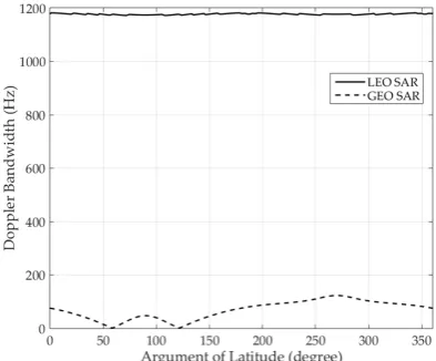
The relationship between azimuth resolution and Doppler bandwidths varies with different targets at different orbit positions. Equations (7) and (10) provide a solution. Using the iterative method to determine the starting observation position (e.g.,S1in Figure5) and ending observing position (e.g.,S2in Figure5) under the predetermined azimuth resolution, the Doppler bandwidths can be obtained by Equation (7). Figure6presents the Doppler bandwidths of GEO SAR and LEO SAR with an azimuth resolution of 5 m. The figure indicates that the Doppler bandwidth of GEO SAR is much smaller than that of LEO SAR, which is caused by the slower relative speed between GEO SAR platforms and targets.

,

Figure 6.Doppler bandwidths of GEO SAR and low earth orbit (LEO) SAR with an azimuth resolution of 5 m based on Equations (7) and (10). We consider L-band GEO SAR in orbit with an inclination angle of 60◦. The parameters employed for LEO SAR are the same as those of L-band ALOS-2 [19]. In this case, the Doppler bandwidth of GEO SAR is nearly 1/10 that of LEO SAR.

3.2. Adjusting the Starting Time of the Receive Window

Remote Sens.2019,11, 17 8 of 26

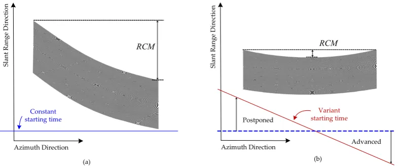
the variable starting time, given by the red line in Figure7b. We note that adjusting the starting time greatly reduces the RCM corresponding to the target, which indicates that the echoes can be recorded using less on-board storage and the range-azimuth coupling decreased. To avoid overlapping between the transmitted pulses and the received signals, the scope for adjusting the starting time must satisfy

∆_ta <_PRT−_{Tp, (11)}

where the pulse repetitive time isPRT= 1/PRF. For LEO SAR with a resolution of 5 m,∆_{tais less than} 0.7 ms [21], which provides no scope for adjusting the starting time. However, the much lower PRF employed with GEO SAR relative to that employed with LEO SAR provides a value of∆taas long as 12 ms, which provides ample scope for adjusting the starting time of the receive window.

RCM

Azimuth Direction

S

la

n

t Ra

n

g

e

D

ir

ec

tio

n

Azimuth Direction

(a) (b)

S

la

n

t Ra

ng

e

D

ir

ec

ti

o

n

Constant starting time

RCM

Postponed

Advanced Variant

starting time

Figure 7.Effect of a variable starting time for the receive window. (a) The echo acquired by the squint mode with a constant starting time for the receive window represented by the blue line. (b) The echo acquired using the same mode but with a starting time that varies according to the red line, where the starting time is postponed during the first half of data recording and is advanced during the latter half.

In this paper, we adjusted the starting time to correct the bulk range walk of the reference target, which is more than 90% of the sum of∆RWand∆RB for an entire swath. Since the range walk is directly defined byr1in Equation (4), the range walk corrected means this item is removed. Therefore, the slant range of a reference target after correction becomes:

Rre f_RWC(t) =r0_re f + 5

∑

rnn

n!t

n_{. (12)}

By comparing Equations (2) and (12), we note that the linear component representing the range migration disappears. Therefore, the adjusted starting timeTS_RWCshould satisfy:

Ts_RWC=Ts_general+2

h

Rre f_RWC(t)−Rre f_act(t)

i

/c, (13)

whereTs_generalis the starting time before adjustment andRref_RWC(t) is the actual range history of the reference target. Furthermore, correcting the bulk range walk on receive ensures thatr1,ref in Equation (3) is equal to 0, which indicates that:

r1=k1,1,r·∆R+k1,1,a|∆R·∆t. (14)

Remote Sens.2019,11, 17 9 of 26

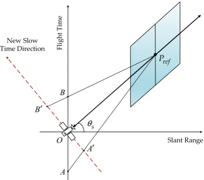
prior to adjusting the starting time of the receive window. By applying Equation (13), the receive time is postponed fromAtoA′or advanced fromBtoB′. As a result, slow time is changed from the flight direction to the new direction denoted by the red dotted line. As such, the deviation between the red dotted line and the flight trajectory complies with Equation (13). The operation makes the new slow time and fast time directions orthogonal, and changes the squint mode to an equivalent broadside mode. However, this change from squint mode to broadside mode is only applicable toPref, and the other targets in the swath are still subject to a slight degree of squint mode observation.



 

 

O

F

lig

h

t T

im

e

Slant Range New Slow

Time Direction

A A′

B

B′

s

θ

ref

P

Figure 8.Equivalence between the broadside mode and the squint mode for a reference targetPrefusing

a variable starting time for the receive window.

4. Squint Imaging Algorithm for GEO SAR after Correcting Bulk Range Walk

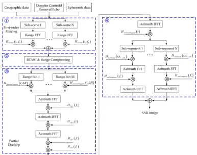
The proposed imaging process comprising operations in the range and azimuth directions after correcting the bulk range walk on receive is illustrated in Figure9. The echo data of four isolated point targets with bulk range walk removed is shown in Figure9a. First-order filtering was applied in the range direction to compensate for the range-dependent termk1,1,r·∆Rin Equation (14), as shown in Figure9b. Then, RCMC and range compression were implemented to obtain the signal illustrated in Figure9c. Next, partial dechirp was used to shorten the span of the aperture time for every target to facilitate the azimuthal segmentation of echoes. The results are shown in Figure9d. Then, azimuth compensation was conducted, which led to the imaging result illustrated in Figure9e. The proposed squint mode imaging algorithm is described by the flowchart given in Figure10. The detailed steps in the algorithm are outlined in the following subsections.

(a) (b) (c) _(d) (e)

Slant Range

F

lig

ht

T

im

e





p



q

r

s

Remote Sens.2019,11, 17 10 of 26

Figure 10.Flowchart for the proposed squint mode GEO SAR imaging algorithm, which is composed of four steps. Step 1 is first-order filtering. Step 2 includes range cell migration correction (RCMC) and range compression. Step 3 implements partial dechirp. Azimuth compensation is accomplished in Step 4.

4.1. Operations in the Range Direction

After transforming Equation (1) into the range frequency domain, the return signal is given as:

SrngF(t,fτ;tc,∆R) =σ·rect

t−tc

Ts

·rect

fτ

Br

·exp

−jπf

2

τ

Kr

·exp

−j4π(fτ+ f0)

c R(t)

, (15)

where fτis the range frequency,Br =KrTpis the bandwidth of the transmitted signal, and f0is the carrier frequency. To increase the accuracy of RCMC, the termk1,1,r·∆R in Equation (14) should first be removed. Because k1,1,r·∆R depends on the position of a target, the return signal must be segmented in the range direction. The length of each segment∆_{Rseg can be 1.5–2 times} ∆_RB. Then, the range-dependent term k1,1,r·∆Rcan be compensated in each segment by the following first-order filter:

HLrcmc=exp

j4π(f0+fτ)

c ·k1,1,r·∆Rseg·t

. (16)

Subsequently, RCMC and range compression are implemented using the fourth-order nonlinear chirp scaling imaging algorithm [22], which extends the RCMC ability in the range direction, and the echo becomes (AppendixA):

S(t,τ;tc,∆R) =σ·rect

_t−t

c

Ts

·sinc τ−τmig·exp

−j4π

λ R(t)

, (17)

Remote Sens.2019,11, 17 11 of 26

4.2. Operation in the Azimuth Direction

Because the signal has been well compressed in the range direction, the azimuth operations can be implemented in each range gate. The first time-scaling given as:

HAS1(t;∆R) =exp

j2π

λ k1,1,a|∆Rt

2 ₍₁₈₎

is used to remove the azimuth-dependent termk1,1,a|∆R·∆tc. Then, the frequency-scaling

HY3Y4(ft;∆R) =exp

(

j2πY3|∆R

3λ

λ 2

3

ft3−j πY4|∆R

λ

λ 2

4

ft4

)

(19)

and the second time-scaling

HAS2(t) =exp

( −j4π

λ · 5

∑

pn

n!t n

)

(20)

are subsequently applied to correct the quadratic and linear spatial variances in rn (n = 3, 4, 5), respectively. Expressions for the undefined parameters in Equations (19) and (20), including Y3, Y4,p3,

p4, andp5, are given in AppendixB. After removing the azimuth spatial variance inrn(n= 3, 4, 5), the higher-order items in the frequency domain can be compensated by applying

Hapc(ft) =exp

( −j4π

λ 10

∑

Pm

λft 2

m)

, (21)

where the values ofPm(m= 3–10) are defined in AppendixC. Implementing Equations (18)–(21) transforms the return signal as follows:

Sapc(t,τ;tc,∆R)≈σ·rect

t−tc

Ts

·sincτ−τ_mig ·exp

−j4π

λ

r0−k1,1,2a|∆Rtc2+12 r2−k1,1,a|∆R

(t−tc)2+ 5

∑

n=3 rn|∆_tc=0

n (t−tc)n

(22)

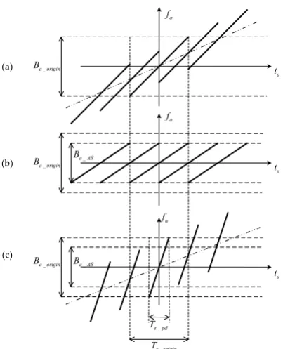
The time-frequency relationships corresponding to Equations (17) and (22) are illustrated in Figure11a,b, respectively. Here, the Doppler bandwidth is transformed fromBa_origin ≈ 2|r2|Ts/λ toBa_AS ≈ 2|r2−k1,1,a|∆R|Ts/λ. However, the Doppler bandwidth must be recovered to preserve the azimuth resolution. This is implemented using partial dechirp, which consists of applying the following two steps:

(

HPD_1(ft) =exp{−j2π·χ·φ0(ft)}

HPD_2(t) =exp

n

−j4_λπ·k1,1,a|∆R

2(1−χ)t2

o (23)

Here,φ0(ft)can be calculated according to Equation (A8) in AppendixA, andχis the partial dechirp coefficient, where 0<χ<1. The application of Equation (23) transforms the echo as follows:

SPD(t,τ;tc,∆R) =σ·rect

h _t

−tc

(1−χ)Ts

i

·sinc τ−τmig

·exp

−j4_λπ

r′0+r′1·(t−tc) +r ′

2

2 ·(t−tc) 2

+ ∑5

n=3 rn,re f|∆R

n (t−tc)

n (24)

Remote Sens.2019,11, 17 12 of 26



 _{ }

  

 



 

  



 

 

 

 

  

 _{ }

 _{ }

 _{ }

 



 

 

 

 

 

 

 

 

 

_

a origin

B

a

t

a

f

a

t

a

f

_ a origin

B Ba_AS

a

t

a

f

_

a origin

B Ba_AS

_

s origin

T

_

s pd

T

(a)

(b)

(c)

Figure 11.Azimuth time-frequency relationships corresponding to Equations (17), (22), and (24) are illustrated in (a–c), respectively.

After conducting partial dechirp, azimuthal segmentation is employed, where the width of each segment is(1−χ)Ts. We can compensate for the azimuth-dependent term in Equation (24) by applying

HsubScene(t;tc,sub) =exp

j4π

λ

k1,1,a|∆Rtc,sub

(1−χ) (t−tc,sub)

(25)

to each azimuth segment, wheretc,subdenotes the center time of each azimuth segment. Once the spatial variance in the azimuth direction has been removed, azimuth compression is implemented by applying:

HaziCompress(ft) =exp

(

−jπλ(1−χ)

2r2|∆tc=0 ft2

)

. (26)

Then, the final imaging result is obtained by transforming the return signal into the 2D time domain.

5. Simulation and Analysis

5.1. Simulation Method and Parameters

Remote Sens.2019,11, 17 13 of 26

|r3|Ts2/8. Due tor2potentially being zero in some AOL positions, we mapped the ratio between these two into a negative exponential function, and introduced the spatial variance index:

gvar=exp

−|r3|

|r2| ·

Ts 4

. (27)

This means that whengvaris closer to 1, the linear component accounts for a larger proportion, and then the spatial variance weakens, and vice versa.

Another key factor dominating the performance of an imaging algorithm is the squint angle. As mentioned before, the squint angle is much smaller in GEO SAR, limited to±8◦, than in LEO SAR. This means that the traditional squint angle, or together with the elevation angle, cannot describe the squint characteristic in GEO SAR. Therefore, the ground squint angle was introduced to evaluate the squint condition in GEO SAR [18], which is the projection angle on ground of the traditional squint angle. The relationship of these angles is demonstrated in Figure12.

 

 

 

 

 

S

N

P s

V 

g

V

g

θ

s

θ

L

θ

Q

Figure 12. The observation angle relationships in GEO SAR.Sdenotes the satellite position,Pis the target position on the ground, andNis the nadir point. SPis the beam-center line. SNQis the zero-Doppler plane,SNPis the squint plane,θ_Lis the elevation angle,θsis the squint angle, andθgis

the ground squint angle.

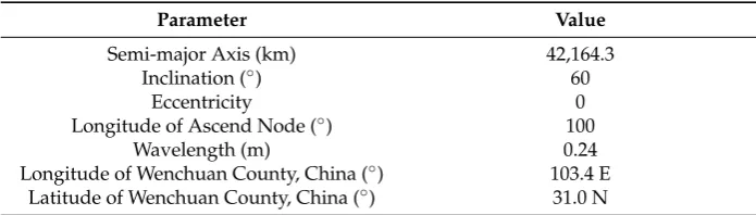
The simulation parameters are listed in Table1. The orbital parameters refer to the Global Earthquake Satellite System (GESS) projection [3]. The swath center is selected as Wenchuan County in China, which is a highly seismic zone requiring frequent observation.

Table 1.Simulation parameters.

Parameter Value

Semi-major Axis (km) 42,164.3

Inclination (◦) 60

Eccentricity 0

Longitude of Ascend Node (◦) 100

Wavelength (m) 0.24

Longitude of Wenchuan County, China (◦) 103.4 E Latitude of Wenchuan County, China (◦) 31.0 N

5.2. Observation Duration Comparison

Remote Sens.2019,11, 17 14 of 26

the nadir trajectory, the red lines represent the feasible observation durations corresponding to the respective observation modes, and the green point represents the target location.

A

B C

D

E F

(a) (b)

Figure 13.Comparison of GEO SAR observation durations obtained for a nadir trajectory mode (a) in broadside and (b) the proposed squint mode method.

For the broadside mode, there are only three positions that can be used to observe Wenchuan, as shown in Figure 13a. The AOLs of three positions are nearly 30◦, 87◦, and 148◦. At these positions, the squint angle and elevation angle, denoted by(θL,θs), should be (1.92◦,2.10◦), (4.82◦,0.51◦), and (0.99◦,−1.56◦). The ground squint angles of these three positions are equal to zero. Applying the broadside mode yields an observation duration of about 0.59 h per orbit, which is 2.47% of the orbital period. In contrast, through adjusting the observing angles in different AOLs, the proposed algorithm can image Wenchuan for several strip areas, as shown in Figure13b. Applying the proposed method, the observation duration increased to about 11.55 h per orbit, which is 48.15% of the orbital period. The results indicate that the proposed method significantly improves the observation ability of GEO SAR.

5.3. Imaging Results and Analysis

Figure13shows the feasible observation period in different modes. There is no need to clarify the feasible period in Figure12a because so many broadside imaging algorithms have that ability. However, the feasible periods in Figure12b were created by the proposed algorithm, which should be verified. In Figure13b, three sections,FA,BC, andDE, are stated as the feasible periods. According to the simulation parameters listed in Table1, we drew the spatial variance indexgvarand ground squint angleθgcurves in the full orbit, which are shown in Figure14.

According to Section5.1, the most difficult position for imaging are among A~F. Therefore, the main characteristics of these points are listed in Table2.

According to Table2, position A has the most severe spatial variance (gvar= 0.955), and position D has the largest ground squint angle (θg= 62.53◦). Hence, if the imaging qualification in A and D can be guaranteed, then all the other positions in the feasible period in Figure13b can be focused well.

Remote Sens.2019,11, 17 15 of 26

A B C D E F

A _B

C D

E

F

(a) (b)

--

--

--

-Figure 14.The spatial variance index and ground squint angle curves when observing Wenchuan in full orbit. (a) The spatial variance indexgvar; (b) the ground squint angleθg. The black dashed line is

the Doppler centroid frequency, which has three intersection points with the ground squint angle curve atθg=0. These three points are highlighted by green circles, corresponding to the broadside mode in

Figure13a.

Table 2.Characteristics of candidate positions.

Index AOL (◦_{) Longitute-Latitude of Nadir (}◦_{) gvar θg(}◦_{) θ}

L(◦) θs(◦) Ts(s)

A 47.10 (81.18E, 39.38N) 0.955 26.95 3.18 1.30 365.08 B 67.29 (82.78E, 53.02N) 0.965 24.48 4.43 0.67 465.53 C 107.66 (114.83E, 55.61N) 0.965 −31.66 4.35 0.37 529.99 D 131.22 (119.07E, 40.65N) 0.959 −39.51 2.74 −0.43 428.13 E 185.05 (97.48E, 4.37S) 0.981 62.53 −3.61 −4.48 714.52 F 343.18 (108.23E, 14.51S) 0.964 −58.63 −4.15 5.52 722.26

Range Direction Azimuth

Direction

1

T

2

T

3

T

30km 30km

Remote Sens.2019,11, 17 16 of 26

and17were evaluated according to resolution (res), peak to side lobe ratio (PSLR), and integrated side lobe ratio (ISLR) along the azimuth and range directions, and the results are presented in Table3. Here, PSLR is defined as the ratio of the peak level of sidelobes to the peak level of the main lobe, and the ISLR is the ratio of the total power in all sidelobes to the power in the main lobe.

(a) (b) (c)

A

zim

u

th (Sam

p

les

)

A

m

p

lit

u

d

e (

d

B

)

A

m

p

lit

u

d

e (

d

B

)

(d) (e) (f)

(g) (h) (i)

Range (Samples)

200 400 600 800 1000

100 200 300 400 500 600 700 800 900 1000

Azimuth (Samples)

1000 2000 3000 4000 5000 6000 7000

A

m

plit

ud

e (d

B

)

-40 -35 -30 -25 -20 -15 -10 -5 0

Range (Samples)

2500 3000 3500 4000 4500 5000 5500 6000

A

m

plit

ud

e (d

B

)

-40 -35 -30 -25 -20 -15 -10 -5 0

Range (Samples)

200 400 600 800 1000

500 1000 1500 2000 2500 3000 3500 4000

Azimuth (Samples) 104

0 1 2 3 4

-40 -35 -30 -25 -20 -15 -10 -5 0

Range (Samples)

2000 2500 3000 3500 4000 4500 5000 5500 6000

A

m

plit

ud

e (d

B

)

-40 -35 -30 -25 -20 -15 -10 -5 0

Figure 16. Imaging results of the 2D nonlinear chirp scaling (CS) algorithm [18]. The first (a–c), second (d–f), and third (g–i) row correspond respectively to pointsT1,T2, andT3illustrated in Figure15.

The first (a,d,g), second (b,e,h), and third (c,f,i) column represent contour maps, azimuth profiles, and range profiles, respectively.

Table 3.Evaluation of imaging quality (in position A).

Azimuth Direction Range Direction

Method Target Res (m) PSLR (dB) ISLR (dB) Res (m) PSLR (dB) ISLR (dB)

Algorithm proposed by Zhang et al. [18]

T1 55.622 −15.129 −19.633 1.578 −12.963 −10.624

T2 4.810 −12.525 −10.279 1.522 −13.279 −10.050

T3 33.486 −0.809 −1.828 1.522 −9.213 −7.721

Proposed Algorithm

T1 4.775 −13.256 −10.295 1.534 −13.351 −10.138

T2 4.800 −13.168 −10.153 1.534 −13.264 −10.039

Remote Sens.2019,11, 17 17 of 26

(a) (b) (c)

(d) (e) (f)

Range (Samples)

200 400 600 800 1000

100 200 300 400 500 600 700 800 900 1000 Azimuth (Samples)

1000 2000 3000 4000 5000 6000 7000

A m plit ud e (d B ) -40 -35 -30 -25 -20 -15 -10 -5 0 Range (Samples)

2000 2500 3000 3500 4000 4500 5000 5500 6000

A m plit ud e (d B ) -40 -35 -30 -25 -20 -15 -10 -5 0 Range (Samples)

200 400 600 800 1000

100 200 300 400 500 600 700 800 900 1000 Azimuth (Samples)

1000 2000 3000 4000 5000 6000 7000

A m p lit u d e ( d B ) -40 -35 -30 -25 -20 -15 -10 -5 0 Range (Samples)

2000 2500 3000 3500 4000 4500 5000 5500 6000

A m plit ud e (d B ) -40 -35 -30 -25 -20 -15 -10 -5 0

(g) (h) (i)

- - - -- - - -- - - -- - - -- - - -- - - -Range (Samples)

200 400 600 800 1000

100 200 300 400 500 600 700 800 900 1000 Azimuth (Samples) 1000 2000 3000 4000 5000 6000 7000

A m p lit u d e ( d B ) -40 -35 -30 -25 -20 -15 -10 -5 0 Range (Samples)

2000 2500 3000 3500 4000 4500 5000 5500 6000

A m p lit u d e ( d B ) -40 -35 -30 -25 -20 -15 -10 -5 0

Figure 17. Imaging results of the proposed squint mode algorithm. Images (a–i) are equivalent representations to those given in Figure16.

The algorithm proposed by Zhang et al. [18] neglects the residual walk after removing the bulk range walk, and this negatively affects the azimuth spectrum of the imaging results, as indicated by Figures16and17and Table3. This issue becomes increasingly serious as the spatial variance increases. As shown in Figure16, the swath center pointT2is well focused. However, for pointsT1and

T3, which are at the edges of the swath, the signal in azimuth is almost defocused. Since the spatial variance is so severe that the traditional nonlinear chirp scaling does not work well, the imaging quality in range direction is degraded. However, the proposed algorithm preserves the focusing performance of the 2D nonlinear CS algorithm over the full scene. From the quality indices presented in Table3, the imaging coherency is good over the entire swath. Since the fourth-order nonlinear chirp scaling is used in range direction, the focusing ability in range direction is improved compared to the algorithm proposed by Zhang et al. [18].

Remote Sens.2019,11, 17 18 of 26

(a) (b) (c)

(d) (e) (f)

(g) (h) (i)

A

zim

u

th (Sam

ples

)

A

m

plit

ud

e (d

B

)

A

m

plit

ud

e (d

B

)

A

zi

m

ut

h

(

S

am

ples

)

A

m

p

lit

ud

e (

d

B

)

A

m

plit

ud

e (d

B

)

A

zi

m

ut

h

(

S

am

pl

es

)

A

m

plit

ud

e (

d

B

)

A

m

plit

ud

e (d

B

)

Figure 18. Imaging results of the proposed squint mode algorithm. Images (a–i) are equivalent representations to those given in Figure16.

Table 4.Evaluation of imaging quality (in position D).

Azimuth Direction Range Direction

Method Target Res (m) PSLR (dB) ISLR (dB) Res (m) PSLR (dB) ISLR (dB)

Proposed Algorithm

T1 4.656 −13.233 −9.695 1.318 −13.298 −10.097 T2 4.866 −13.310 −10.253 1.309 −13.233 −10.031 T3 4.952 −13.158 −10.250 1.318 −13.324 −10.139

Remote Sens.2019,11, 17 19 of 26

6. Discussion

6.1. Accuracy

In order to correct the squint effect, the linear residual terms k1,1,r·∆R andk1,1,a|∆R·∆tc in Equation (3) were removed since these two terms depend on the locations of targets. Segmentation was adopted by applying Equations (16) and (25). After segmentation, each sub-block corresponds to an area of∆_{Rseg×(1−χ)Ts, as shown in Figure19. When processing each sub-block of data,} the follow-up filters were designed according to the center pointPC. Therefore, for all points except

PC, residual phase errors occur, which have to be controlled to guarantee the imaging accuracy.

ΔR_seg

()

χ

−

1

s

T

M P

C P Slant Range

A

z

im

ut

h

   

   

   

  _{ } 

  _{ } 

 _{ }

 _   _

 



Figure 19.Points in one sub-block diagram. PointPCis located at the sub-block center, whereasPMis

a set denoting every point at the corner.

Suppose a target located at(∆_t,∆_{R)has an accurate 2D frequency domain phase}Φa₍∆_t,∆_R) and the polynomial expansion phaseΦe₍∆_t,∆_{R). In some positions where the spatial variance is} minimal, the range walk removed echo data are like broadside data, which means r1 ≈ 0 and Φa _≈Φe. However, for some severe spatial variant areas,k1,1,r·∆Randk1,1,a|∆R·∆tcchange drastically. The expansionΦe₍∆_t,∆_{R)is no longer accurate. Segmentation can be used to correct it. Therefore,} the correct approach to weigh the segmentation is to improve the quality of the phase error of the corner points. That is,

∆Φ χ,∆Rseg/∆RB=max P∈PM

Φe_P

∆t±Ts

2(1−χ),∆R± 1 2∆Rseg

−Φa_P

∆t±Ts

2(1−χ),∆R± 1 2∆Rseg

, (28)

where

 



Φa₍∆_t,∆_{R) =−}4π(fτ+f0) c

r0−

9 ∑ n=1

An

n+1

− c ft

2(f0+fτ)−r1 n+1

Φe_{(∆t,∆R) =Φ(ft,f}

τ)

, (29)

and the∆_tand∆_{Rare inherent inrnandAn, which are defined in Equations (3) and (A9).}Φ_(ft,fτ)is shown in Equation (A7).

The relative phase∆Φ _{should be controlled at a very low level, which means segmentation} contributes to an accurate expression without introducing phase error. To this end, Equation (28) should obey

∆Φ _χ,∆Rseg/∆RB< π

4M, (30)

whereM> 1 is an adjustable coefficient.

Remote Sens.2019,11, 17 20 of 26

introduce error by this means. Using the simulation examples demonstrated in Section5, the simulated relationship among∆_{Rseg,χ, and}∆Φ_{is demonstrated in Figure20.}

(a) (b)

Figure 20.The simulated relative phase∆Φ_againstχand∆_{Rseg. (}a) and (b) correspond to targetsT3in

position A and position D in Table2, respectively. These two images reflect the corner points’PMphase

error of controlled by∆Rsegandχ.∆Φheavily relies onχ, which means the azimuth spatial variance is

more severe than in the range direction. This was verified by imaging results in Figure16g,h. From the simulation results,χshould be larger than 0.8, whereas∆_{Rsegcan be several times}∆_{RBwith high}∆Φ

values avoided.

The final imaging quality does not depend on Equation (30); instead, quality depends on the fourth-order NCS in range direction and time-frequency scaling in the azimuth direction. Equation (30) only ensures that segmentation has no effect on the subsequent image quality. Since the fourth-order NCS and time-frequency are designed for imaging a broad scene, the imaging quality of targets in small 30×30 km areas can be ensured in most circumstances. This means that the marginal points of sub-blocks can be focused. The error between sub-blocks can only be distorted, which can be resolved by geometric calibration before stitching.

6.2. Computational Load

The computational load is one of the main factors affecting the practical application of the algorithm. To multiply a pair of complex numbers requires six floating point operations per second (FLOPs), whereas only one FLOP is needed for complex addition. Specifically, creating anNpoints FFT (or IFFT) operation requires 5Nlog2(N) FLOPs [20]. Suppose the echo data hasNaziandNrngsampling points in the azimuth and slant range directions, respectively, after range walk removal. For the BP algorithm, with eight-times interpolation in the range direction, and imaging an area ofNrng×Nrng size, the computational load of BP is:

CBP =45NaziNrnglog₂ Nrng+7NaziNrng2 . (31)

However, for the algorithm proposed, there are 4NazitimesNrngpoints FFT operations, 10Nrng timesNazipoints FFT operations, and 14NaziNrngtimes multiplications. Therefore, the computational load is:

Cp≈20NaziNrnglog₂ Nrng+50NaziNrnglog₂(Nazi) +84NaziNrng. (32)

Remote Sens.2019,11, 17 21 of 26

for practical use. In addition, many segmenting operations exist that can be easily used by parallel computing. This further shortens the time required for the method when implementing in modern computers.

7. Conclusions

We proposed a novel squint mode GEO SAR imaging method, where the bulk range walk is first corrected on receive by adjusting the starting time of the receive window and then applying first-order filtering, RCMC, range compression, partial dechirp, and azimuth compression to obtain the focused single looking complex (SLC) image. Simulation results demonstrated that the proposed algorithm achieves a resolution less than 5 m in the azimuth direction over a 30×30 km swath.

In addition to the performance, the feasibility of the proposed algorithm was investigated. Firstly, up-to-date technology can make the antenna have the ability to scan in a range of±8◦ in the azimuth direction, which indicates that the staring mode can be realized. Secondly, the low PRF employed with GEO SAR provides ample scope for adjusting the starting time of the receive window and removing the range walk on receive. Lastly, the ephemeris data and geographic information of the target zone can be acquired to calculate the coefficients of the range model and each filter in the proposed algorithm, and focused imaging results can be produced.

The staring mode of GEO SAR enables the continuous observation of the region of interest. Compared with the broadside mode, the proposed method increases the observation duration for Wenchuan County in China by nearly 20 times. As a result, the proposed method enables GEO SAR to conduct long-term observation of target zones, which is essential for the management of global disasters and related affairs. For earthquake-prone areas, like Wenchuan, the starting mode can continuously provide images over a long time period after an earthquake. Some disaster information, including dammed lakes, landslides, and mudslides, can be updated continuously, which is central to disaster relief and rescue.

Another distinctive characteristic of GEO SAR is the short temporal resolution, which is vital to the application of interferometry, such as vegetation measurement and crust deformation detection. However, interferometry cannot be realized by applying several images obtained at different squint angles within one orbit period and coherent change detection needs to use the same observation geometry. For this reason, for interferometric applications, it is necessary to wait at least one orbit period (one day), similarly to the polar orbit repeat pass interferometry case.

Author Contributions:All authors contributed equally to this paper in ideas, design of methodology and writing. Additionally, Z.Y. was responsible for project administration, data analysis and experiments validation, writing. J.G. accomplished software programming, data analysis and presentation.

Funding:This research was funded by China Scholarship Council (Grant No. 201706025038).

Acknowledgments:This work was supported by the Program of the China Scholarship Council under Grant No. 201706025038.

Conflicts of Interest:The authors declare no conflicts of interest.

Appendix A.

Application of the first-order filter in Equation (16) removes the residual range-Doppler component k1,1,r ·∆R in Equation (14). Then, Equation (15) is multiplied with the following scaling function:

HAS1(t,fτ) =exp

−j4π(fτ+f0)

c rpt(t)

, (A1)

Remote Sens.2019,11, 17 22 of 26

Therefore, at this stage, cubic perturbation factorYand quartic perturbation factorZwere also inserted. Subsequently, the echo was transformed into the 2D frequency domain represented by the azimuth frequencyftand the range frequencyfτ, and compensated for by multiplying with:

H3plus_Y(ft,fτ) =exp (

−j2π 9

∑

φk,re f(ft)· fτk )

·exp

j2π

1 3Y·f

3

τ+

1 4Z· f

4

τ

, (A2)

whereφk,re f(ft)are the frequency coefficients of the reference target. The expressions forφk,re f(ft) are provided in TableA1. YandZare defined in (A11), at the end of this appendix. According to a previous study [22], the nonlinear CS function is designed as

HNCS(ft,τ) =exp

−jπQ2

τ−τre f

2 −j2π

3 Q3

τ−τre f

3 −jπ

2Q4

τ−τre f

4

, (A3)

whereτre f is the position of the reference target in the range-Doppler domain, andQ2,Q3, andQ4are

ft-dependent scaling coefficients, which are defined in Equation (A11). After conducting the scaling operation, all targets have an equivalent RCM, which can be corrected by multiplying the echo with:

Hrpc_rcmc(ft,fτ) =exp

−jπ

2 3

YK3

mre f+Q3

(Kmre f+Q2)

2fτ3+K_{mre f}1+Q2f 2

τ

·exp

−jπ₂ ·2(Jmre f+Q3)2−(Lmre f+Q4)(Kmre f+Q2)

(K_{mre f}+Q2)5

·f4

τ

·expnj2πfτ h

φ1,re f

ft,re f

−φ1,re f(ft)

io

(A4)

The first and second exponential terms are applied for range compression, whereas the third exponential term is applied for correcting the bulk RCMC.Kmref,Jmref, andLmrefare the frequency quadratic, cubic, and quartic modulation of the reference target in the range-Doppler domain respectively, which is defined in Equation (A11). After this operation, the RCM values of all targets have been corrected, and the residual phase can be compensated by multiplying the echo with:

Hresidual(ft) =exp

jπKmre f +Ks1·τ′+Ks2·τ′2

α·τ′+β·τ′22

·exp

−j2₃πJmre f+Js1·τ′

α·τ′+β·τ′23

·exp

jπ₂Lmre f

α·τ′+β·τ′24

·expnjπhQ2·τ′2+23Q3·τ′3+12Q4·τ′4

io

(A5)

where τ′ = τ−2r0,re f/c and Ks1 and Ks2 are the linear and quadratic coefficient of frequency modulation, respectively, which are defined in Equation (A11). Js1 is the linear coefficient of cubic modulation, and α and β are the linear and quadratic scaling parameter, respectively, which can be obtained by traditional NCS method. The specific expression is also in Equation (A11). Here, the time-scaling operations in Equation (A1) have changed the spatial variance in the azimuth direction. Therefore, to facilitate azimuth processing, it was necessary to recover the spatial variance at each range bin by applying the filter

H_AS1(t) =exp

j4π

λ rpt(t)

. (A6)

Remote Sens.2019,11, 17 23 of 26

Lastly, the specific expressions of the parameters given in Equations (A2)–(A5) are listed here. First, the 2D frequency domain phase is expanded in the following series form:

Φ_{(ft,fτ)≈2πφ0(ft) +2π} 9

∑

φn(ft)· fτn, (A7)

where the coefficientsφn(ft)(n=0−9)are defined as follows:

                      

φ0(ft)≈φ0,re f(ft) +M1,r(ft)·∆R+M2,r(ft)·∆R2+M1,a(ft;∆R)·∆t

+M2,a(ft;∆R)·∆t2+M3,a(ft;∆R)·∆t3

φ1(ft)≈φ1,re f(ft) +L1,r(ft)·∆R+L2,r(ft)·∆R2+L1,a(ft;∆R)·∆t

+L2,a(ft;∆R)·∆t2

φ2(ft)≈φ2,re f(ft) +J1,r(ft)·∆R+J1,a(ft;∆R)·∆t+J2,a(ft;∆R)·∆t2 φ3(ft)≈φ3,re f(ft) +K1,r(ft)·∆R+K1,a(ft;∆R)·∆t

φk(ft)≈φk,re f(ft), 4≤k≤9

. (A8)

This is the spatial mode of the 2D spectrum, and the specific expressions employed herein are listed in TableA1.

Table A1.Spatially variant coefficients in the 2D frequency domain.

φ0(ft) φ1(ft)

                                        

φ0,re f(ft) =−2r0,_λre f +

10

∑ m=2

Am−1,re f

m

−λft

2

m

M1,r(ft) =−_λ2+

10

∑ m=2

lm−1,1,r

m

−λft

2

m

M2,r(ft) = 2_λ

10

∑ m=2

lm−1,2,r

m

−λft

2

m

M1,a(ft;∆R) = 2_λ

10

∑ m=2

lm−1,1,a

m

−λft

2

m

M2,a(ft;∆R) = 2_λ

10

∑ m=2

lm−1,2,a

m

−λft

2

m

M3,a(ft;∆R) = 2_λ

10

∑ m=2

lm−1,3,a

m

−λft

2 m                                 

φ1,re f(ft) =−2r0,_cre f−_λ2

10

∑ m=2

Am−1,re f

m (m−1)

−λft

2

m

L1,r(ft) =−2c−λ2

10

∑ m=2

lm−1,1,r

m (m−1)

−λft

2

m

L2,r(ft) =−2c

10

∑ m=2

lm−1,2,r

m (m−1)

−λft

2

m

L1,a(ft) =−2c

10

∑ m=2

lm−1,1,a

m (m−1)

−λft

2

m

L2,a(ft) =−2c

10

∑ m=2

lm−1,2,a

m (m−1)

−λft

2

m

φ2(ft) φ3(ft)

                        

φ2,re f(ft) =−21Kr+

2

c f0

10

∑ m=2

Am−1,re f

m C2m

−λft

2

m

J1,r(ft) = _{c f}2₀

10

∑ m=2

lm−1,1,r

m C2m

−λft

2

m

J1,a(ft;∆R) = _{c f}2₀

10

∑ m=2

lm−1,1,a

m Cm2

−λft

2

m

J2,a(ft;∆R) = _{c f}2₀

10

∑ m=2

lm−1,2,a

m Cm2

−λft

2 m               

φ3,re f(ft) =−_{c f}22 0

10

∑ m=2

Am−1,re f

m Cm3+1

−λft

2

m

K1,r(ft) =−_{c f}22 0

10

∑ m=2

lm−1,1,r

m C3m+1

−λft

2

m

K1,a(ft) =−_{c f}22 0

10

∑ m=2

lm−1,1,a

m C3m+1

−λft

2

m

φk(ft), 4≤k≤9

φk,re f(ft) = (−1)k2_c

10

∑ m=2

Am−1,re f

m Cmk+k−2

−λft

2

m

Remote Sens.2019,11, 17 24 of 26                     

A1=1/r2

A2=−r3/2r32

A3= 3r32−r2r4/6r5₂

A4=− r22r5+15r33−10r2r3r4

/24r7₂

A5= 10r22r42−r23r6+105r2r23r4−105r2r23r4+15r22r3r5/120r92

A6=− r24r7−21r32r3r6−35r23r4r5+210r22r23r5+280r22r3r42−1260r2r33r4+945r53

/720r11₂

· · ·

(A9)

In addition,{lm,1,r,lm,2,r,lm,1,a,lm,2,a,lm,3,a}are the spatial coefficients, which can be resolved by numerical analysis according to the function

Am=Am,re f+lm,1,r·∆R+lm,2,r·∆R2+lm,1,a·∆t+lm,2,a·∆t2+lm,3,a·∆t3. (A10)

Expressions for the parameters related to CS in Equations (A2)–(A5) can be determined according to a previously proposed method [21], and are given as follows:

                                                                

Kmre f =1/

2φ2,re f

Ks1=2K2mre fJ1,r(ft)/L1,r

fre f

Ks2=

h

4K3

mre fJ1,r2 (ft)−2Kmre f2 J2,r(ft)

i

/L2 1,r

fre f

+2K2

mre fJ1,r(ft)L2,r

fre f

/L3 1,r

fre f

Jmre f =

h

2βKmre f + (2α+1)Ks1

i

/2α(α+1)

Js1=

h

6J1,r(ft)·Jmre f·Kmre f−3K1,r(ft)·K3_{mre f}

i

/L1,r

fre f

Lmre f =

h

(2α+1)Js1+2Jmre fβ−Ks2

i

/3α(α+1)

α=L1,r(ft)/L1,r

fre f

−1

β=hL1,r(ft)L2,r

fre f

−L2,r(ft)L1,r

fre f

i

/L3_1,rfre f

Y=Jmre f/K_{mre f}3 −3φ3,re f

Z=2J2

mre f −Lmre fKmre f

/K5 mre f

Q2=αKmre f

Q3=

0.5αKs+βKmre f

/(1+α) Q4=αLmre f−Js1/3

(A11)

Appendix B.

In Equations (19) and (20), the parametersY3,Y4,p3,p4, andp5 can be derived according to a previous study [16] as follows:

Y3= 1

4k2,1,a· r2|tc=0

3 h

−k2_2,1,a−r3|tc=0·k2,1,a−(2k2,2,a+3k3,1,a)·r2|tc=0

i

(A12)

Y4=−

1 60k2_2,1,a r2|tc=0

5        

12k2_2,1,a· r3|tc=0

2

−15k2_2,2,a· r3|tc=0

2

−21k3_2,1,a·r3|tc=0 +9k4_2,1,a−24k2_2,1,a·k2,2,a·r2|tc=0+11k

2

2,1,a·k3,1,a·r2|tc=0

−6k2,1,a·k3,2,a· r2|tc=0

2

−6k2,2,a·k3,1,a· r2|tc=0

2

−2k2_2,1,a·r2|tc=0·r4|tc=0+30k2,1,a·k2,2,a·r2|tc=0tc=0·r3|tc=0

−12k2,1,a·k3,1,a·r2tc=0·r3|tc=0

        (A13)

p3=−k2,1,a|∆R (A14)