ALAN HEPBURN WELSH
A THESIS SUBMITTED FOR THE DEGREE OF DOCTOR OF PHILOSOPHY
OF
THE AUSTRALIAN NATIONAL UNIVERSITY
DECLARATION
I he re by c e r t i f y t h a t t h i s t h e s i s does n o t c o n t a i n any m a t e r i a l p r e v i o u s l y p u b l i s h e d or w r i t t e n by any o t h e r person e x c e p t where due r e f e r e n c e i s made in t h e t e x t .
CONTENTS
DECLARATION i .
CONTENTS i i .
PREFACE v .
1 . THE FUNCTIONAL LEAST SQUARES PROCEDURE
1 . 1 I n t r o d u c t i o n 1 .
1 . 2 A s y m p t o t i c t h e o r y 5 .
1 . 3 An a n g u l a r i n t e r p r e t a t i o n 1 3 . 1 . 4 I n t e r c e p t e s t i m a t i o n 1 5 .
1 . 5 R o b u s t n e s s 2 1 .
1 06 C o m p u t a t i o n o f f u n c t i o n a l l e a s t s q u a r e s e s t i m a t e s 2 6 .
A p p e n d i x 1 2 8 .
2 . THE ESTIMATION OF AUTOREGRESSIVE PROCESSES
2 . 1 I n t r o d u c t i o n 2 9 .
2 . 2 S t r o n g c o n v e r g e n c e r e s u l t s 3 0 .
2 . 3 A g e n e r a l r e s u l t 3 4 .
2 . 4 Weak c o n v e r g e n c e r e s u l t s 3 9 . 2 . 5 F i n i t e s a m p l e e f f i c i e n c y 4 4 .
3.
THE ESTIMATION AND TESTING OF CONSTRAINED LINEAR MODELS
301
Introduction
51.
3.2
Strong convergence r e s u l t s
53.
3.3
Weak convergence r e s u l t s
54.
3.4
Singular design matrices
61.
3 05
Hypothesis t e s ti n g
65.
3.6
The a l t e r n a t i v e hypothesis
72.
Appendix 3
78.
4. THE ESTIMATION OF MULTIVARIATE MODELS
4.1
Introduction
79.
4.2
The singular estimator
82.
4.3
The functional l e a s t squares estimator
88.
4.4
Adaptive estimation
93.
4.5
Multivariate au toregressive processes
99.
406
The mink-muskrat s e r i e s
104.
Appendix 4
106.
5. TESTING GOODNESS-QF-FIT
5.1
Introduction
107.
5.2
A t e s t for departures from symmetry
io9.
5.3
A t e s t for departures from normality
113.
5.4
A t e s t for l o n g - t a i l e d departures from normality
122.
6 . THE ESTIMATION OF PARAMETERS OF REGULAR VARIATION
6 o l I n t r o d u c t i o n 133.
6 . 2 E s t i m a t o r s b a s e d on t h e e m p i r i c a l c h a r a c t e r i s t i c f u n c t i o n 135. 6 . 3 B e s t a t t a i n a b l e r a t e s o f c o n v e r g e n c e 140. 6 . 4 The g o o d n e s s - o f - f i t a p p r o a c h t o d e t e r m i n i n g r Q 148.
6 . 5 A d a p t i v e e s t i m a t i o n 154.
6 . 6 S i m u l a t i o n r e s u l t s 1 61.
PREFACE
This th e s is i s concerned w ith the a p p l i c a t io n o f a d a p tiv e procedures to several s t a t i s t i c a l problems in which the unknown t a i l behaviour o f the u n d e rly in g d i s t r i b u t i o n i s o f im portance.
A daptive techniques are bro ad ly a p p lic a b le to no n-p a ra m etric problems : these techniques p e rm it the c o n s tr u c tio n o f procedures which do n o t depend s u b s t a n t i a l l y on unknown fe a tu re s o f the u n d e rly in g d i s t r i b u t i o n and which may be " e f f i c i e n t " over a broad class o f d i s t r i b u t i o n s . Moreover, r a t h e r than merely a d ju s t in g f o r the unknown t a i l s t r u c t u r e o f the u n d e rly in g d i s t r i b u t i o n , we may a lso be able to p r o t e c t a g a in s t i t and in t h i s sense a d a p tiv e
procedures may a ls o be ro b u s t. We begin t h i s th e s is by c o n s id e rin g the a p p l i c a t io n o f a d a p tiv e e s tim a tio n techniques to l i n e a r ( i . e . re g re s s io n , experimental design and a u to re g re s s iv e ) models w it h
l o n g - t a i l e d e r r o r d i s t r i b u t i o n s . The e v a lu a tio n o f the t a i l s t r u c t u r e o f the e rro rs i s secondary to a d ju s tin g f o r and p r o t e c t in g a g a in s t t h a t s t r u c t u r e and any e v a lu a tio n o f t h a t s t r u c t u r e i s c a r r ie d o u t i m p l i c i t l y d u ring e s tim a tio n . However, a d ap tiv e procedures may
suggest techniques f o r making e x p l i c i t infe re n c e s about the u n d e rly in g t a i l s t r u c t u r e and v ic e v e rsa . Hence, in the l a t t e r p a r t o f t h i s t h e s i s , we c o n sid e r both the problem o f t e s t i n g f o r g o o d n e s s - o f - f i t and o f m o delling the t a i l o f a d i s t r i b u t i o n . In both cases, a d a p tiv e
techniques are a p p r o p r ia t e .
The c la s s i c a l approach to non-param etric problems in v o l v i n g the t a i l s t r u c t u r e o f the u n d e rly in g d i s t r i b u t i o n is through the extreme o rder s t a t i s t i c s . However, i t i s known t h a t the t a i l behaviour o f a d i s t r i b u t i o n f u n c tio n is r e f l e c t e d in the behaviour o f the
This relationship between t a i l s and characteristic functions
pervades this thesis, providing a strong central theme. Of course,
the choice of approach depends on the problem under consideration.
Here we will mainly concentrate on the empirical characteristic
function approach although in the l a s t chapter we will advocate a
technique based on the order s t a t i s t i c s .
In the f i r s t part of this thesis we consider the application of
an adaptive empirical characteristic function technique to linear
model problems. The procedure, called functional le ast squares, is
described in chapter 1. The relationships between functional le ast
squares, le ast squares, angular estimation and M-estimation are
discussed in detail. In addition, the known asymptotic theory of
the procedure is described and the essential conditions stated. The
intercept (location) problem is considered and asymptotic results are
obtained. Finally, a general scheme for the computation of functional
le ast squares estimates is givenG
In the second chapter, the
functional least squares procedure is applied to the problem of
estimating autoregressive processes with long-tailed error distributions.
The asymptotic results include a general result on strong uniform
convergence which is needed in the sequel. The chapter concludes
with a simulation study to investigate the relative efficiency of
the procedure in small samples.
The estimation and testing of constrained linear models is
considered in the third chapter. The general theory leads to a
method of overcoming a singular design matrix and several tests of
hypotheses. In the fourth chapter, the problem of estimating
multivariate linear models is considered. Two generalisations of
the functional le a st squares procedure are considered; one of these
is shown to be an appropriate generalisation.
Indeed, an adaptive
multivariate autoregressive models. An important general result on the
invertibil ity of multivariate autoregressive models is established.,
Finally, the procedure is used to analyse two series of data which
are the annual trappings of mink and muskrat in Canada from
1848-1909.
The l a s t two chapters of this thesis are concerned with the problem
of evaluating the ta il structure of the underlying distribution.
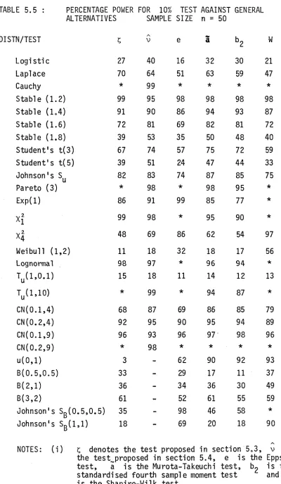
In chapter 5, we derive tests for symmetry and normality. The tests
are based on the empirical characteristic function and are closely
related to the functional least squares procedure. Some
characterisation results are discussed and both the asymptotic theory
and small sample power of the tests are investigated. In chapter 6,
we propose a general non-parametric model for the regularly varying
t a i l s of a distribution and consider the problem of estimating the
parameters of the proposed model. Estimators based on the empirical
characteristic function are constructed and are shown to be inferior
to other estimators based on the extreme order s t a t i s t i c s . These
l a t t e r estimators are shown to attain optimum rates of convergence.
Two approaches to adaptive estimation are considered. Only one of
these approaches is appropriate and we conclude the thesis with a
brief investigation of the small sample properties of this technique.
Section 5.4 and chapter 6 are the product of jo in t work with
Dr P.G. Hall.
Several papers based on the results presented in this thesis have
already been published or submitted for publication. These include
Heathcote and Welsh (1983, 1984), Hall and Welsh (1983, 1984a, 1984b)
and Weish (1983).
I wish to express my sincere gratitude to the members of my
supervision committee, Professor C.R. Heathcote, Dr. P.G. Hall and
throughout the course of this research.
I also wish to acknowledge
my debt to the work of Professor Sc Csörgo and to thank him for his
helpful correspondence. The assistance of a Commonwealth Post-Graduate
Research Award which supported my research was appreciated. Special
thanks are due to Ms0 J. Wilson for her typing of the manuscript.
Finally, I wish to record my deep gratitude to my parents and my wife,
Mary, for her continuing support and encouragement.
Note added in proof:
After the typing of this thesis was completed,
Professor Csörgo pointed out to the author that the discussion at
the bottom of page 10 is contained in his paper "Testing for linearity"
THE FUNCTIONAL LEAST SQUARES PROCEDURE
1.1 I n t r o d u c t i o n
C o n s id e r th e s ta n d a rd l i n e a r r e g r e s s io n model
(1.1.1) Y . = a + x '.$ + e . ,
J J J 1 < j < n , where th e x . = ( x . , , . . . , x . ) ' a re known p - v e c t o r s (p > 1) ,
J j J- J p ”
( a ,8 V i s a ( p + l ) - v e c t o r o f param eters to be e s tim a te d from th e n > p o b s e rv a tio n s Y ^ , . . . , Y n and th e e^. a re in d e p e n d e n tly d i s t r i b u t e d as e . Chambers and H e a th co te (1981) proposed a method o f e s t im a t in g th e s lo p e 8 in ( 1 . 1 . 1 ) which H e ath co te (1982) su b s e q u e n tly
c a l l e d f u n c t i o n a l l e a s t s qua re s. S p e c i f i c a l l y , f o r each t in a s e t T near th e o r i g i n , th e f u n c t i o n a l l e a s t squares e s t im a t o r 8n ( t ) o f 8 a t t i s th e s t a t i s t i c m in im is in g
- 2 -1 ^
( 1 . 1 . 2 ) L ( 8 , t ) = - t n o g |n 1 2 e x p { i t ( Y . - x 3) } | 2 .
n j = l J J
M in i m i s a t io n o f L ( 8 > t ) le a d s to a f a m i l y o f e s t im a t o r s indexed by t e T and a p a r t i c u l a r member o f t h i s f a m i l y may be s e le c te d
a d a p t i v e l y . We w i l l c a l l both th e members o f th e f a m i l y {§ ( t ) , t e T} and any a d a p t i v e l y s e le c te d member o f th e f a m i l y f u n c t i o n a l l e a s t
squares e s t i m a t o r s , a l l o w i n g th e c o n t e x t t o d i s t i n g u i s h between th e two cases.
F u n c tio n a l l e a s t squares was proposed by Chambers and H e ath cote (1981) as an e x te n s io n o f l e a s t squares m ethodology. I f
empirical version of
a2.
I f the error d is trib u tio n lacks a variance
then cle a rly d iff ic u lt ie s arise. Chambers and Heathcote proposed the
loss function (1.1.2) as the empirical version of
(1.1.3)
L (t) = -t~ 2 log |<j>(t)|2 ,
where 4>(t) = u (t) + iv ( t)
is the cha ra cte ristic function of e .
In
the f in it e variance case, as t -* 0 ,
L (t) =
a2+ o (t) ;
moreover, i f
eis normally d istrib u te d L (t) =
a2. Thus least
squares estimation involves minimising the leading term in the
expansion of L ( t) . However, even i f the error d is trib u tio n lacks a
variance L (t)
is well defined fo r a ll
t
f0 such that
|6 (t)| > 0
and in the f i r s t instance i t is th is observation which indicates that
the procedure might have desirable properties.
The intercept term a in the model
(1.1.1)
is not estimable
by functional least squares because the loss function is a function of
the data only through the symmetrised pairs of differences of
residuals rather than through the residuals themselves. We c la r ify
both th is point and the relationship between functional least squares
and least squares by examining the estimating equations.
Following
Chambers and Heathcote (1981) put
-1 n
U (3 ,t) = n
Z cos(t(Y .- x '.3)) ,
n j = i J J
(1.1.4)
n
V (ß ,t) = n
2 s in {t(Y .-x '.ß )}
n
j= l
J J
and w rite (1.1.2) as
Ln(ß ,t) = -t~ 2 log UJ2(ß,t) + V 2 (ß ,t)} .
zero, we obtain
i 1 n - 1 n
t [U ( 3 , t ) n
£ x.sin{t(Y .-x'.ß)} - V ( 3 , t ) n
Z x .
n
j=l J
3 3
n
j = l J
x
cos{t(Y .-x'.3)}] = 0
U vJor, more concisely,
i o " n( 1.1 .5)
t n
Z
Z x.sin{t(Y .-Y. ) - t ( x .-X. ) '3> = 0 .
j =l k=l
3
3
K
J
k
A straightforward argument shows t h a t (1.1 .5 )
holds i f and only i f
1
o n
n
t n
Z
Z (
x .-x.
)
si n
{t( Y .-Y. ) - 1(
x
.
- x
. ) ' 3} = 0 ,
j_-j ^_i j k J K J k
and the l e f t hand side c l e a r l y depends only on pairs of differences
of the r es id ual s and pairs of differe nc es of the x ' s .
Moreover,
in the l i m i t as
t -> 0 ,
( 1. 1. 5)
reduces a f t e r some manipulation to
_ 1
n
i n
(1.1.6)
n
Z (x . - x ) ( x . - x ) '3 = n
Z (x.-x)(Y.-Y) .
j= l J
J
j=l J
J
That (1.1.6)
i s rel a te d to the normal equations for 3 is c le ar
but i t is important to bear in mind t h a t these normal equations
a r i s e from the model
(1.1.1)
with an a t l e a s t i m p l i c i t i n te r c e p t
term r a t h e r than from the regression through the origin model.
S p e c i f i c a l l y , the l e a s t squares estimates for a regression through the
or igin s a t i s f y the equations
-1 n -1
n
n
Z x . x '3 = n
Z x .Y. ,
j =^ J J j = ] 1 1whereas, the l e a s t squares estimates f o r (1 .1.1)
s a t i s f y
a = y - x 3
n
J
n
,
n_i Z x . ( Y . - a - x ' . 3 ) = 0
and on s u b s titu tin g the f i r s t equation in to the remaining equations
( 1 .1 .6 ) is obtained. F i n a lly , Heathcote (1982) has shown th a t i f
A
t f 0 , then 3 ( t ) can be regarded as a perturbed form of
A A
3 = 3 0 .
n n
Thus f a r we have advanced the fu n c tio n a l le a s t squares procedure
merely as a convenient non-parametric g e n e ra lis a tio n o f le a s t squares
which is a p p lica b le to regression models with lo n g - ta ile d e rro r
d i s t r ib u t i o n s . However, the most a t t r a c t i v e fe a tu re o f the method is
the f l e x i b i l i t y i t a ffo rd s when applied a d a p tiv e ly . Under appropriate
c o n d itio n s , the asymptotic variance o f (a p p ro p ria te ly standardised -
see Theorem 1.2) ß ( t ) is a scala r fu n c tio n a2( t ) m u lt ip lie d by a
constant m a trix . The fu n c tio n c 2( t ) is c a lle d the variance fu n c tio n
by Chambers and Heathcote (1982) who suggested minimising an estimate / \
o f o2( t ) to s e le c t an estim ator from the fa m ily (3 ( t ) , t e T} .
They showed th a t
(1 .1 .7 ) g2( t ) = [ u 2( t ) { l - u ( 2 t ) > - 2 u ( t ) v ( t ) v ( 2 t ) + v 2( t ) { l + u ( 2 t ) } ]
/ { 2 t 2 14>( t ) | 4}
and th a t of the d i s t r ib u t i o n s which are normal or le p t o k u r t ic ( i . e .
1o n g e r-ta ile d than normal), the normal is the only one f o r which
a2( t ) is minimised a t t = 0 . Chambers and Heathcote suggested
estim ating o2( t ) by a 2( t ) , defined by replacing u( k t) and
v ( k t) in (1 .1 .7 ) by Un(§n( t ) , k t ) and Vp(3n( t ) , k t ) , k = l,2 ,
re s p e c tiv e ly where U ( 3 , t ) and Vn( 3 , t ) are defined by (1 .1 .4 ) .
Let t denote the minimum o f a2( t ) . Then i f t n + 0 , suspected
o u t lie r s (n^ of them say, n^ < n) may be removed from the sample
and the trimmed sample o f n^ = n-n^ observations reanalysed. Here
and in the sequel, we de fin e o u t l i e r s to be observations which appear
zero then le a s t squares may be deemed a p pro pria te. On the other hand,
i f t is not close to zero then the deleted data points are not
n 2
l i k e l y to be o u t lie r s (with respect to a sample o f normally
d is t r ib u t e d observations) and the recommended estim ator is 3 ( t ) .
Chambers and Heathcote (1981) and Heathcote (1982) discuss graphical
methods to aid in the above a n a ly s is .
1.2 Asymptotic theory
We assume th a t our regression problem (1 .1 .1 ) is embedded in an
i n f i n i t e sequence o f s im ila r problems such th a t the number n o f
observations tends to i n f i n i t y . Chambers and Heathcote (1981)
developed the asymptotic theory o f the estim ator 3 ( t ) f o r each fix e d
t iE T and Csörgo (1983) developed the theory f o r the adaptive
e stim ator. In t h is section we examine t h is theory.
Formally we de fin e the fu n c tio n a l le a s t squares estim ator 3 ( t )
by the equation
(1 .2 .1 ) L ( 3n( t ) , t ) = i n f L ( 3 , t ) , t e T
n n 3 g B
where L ( 3 »t ) is defined by (1 .1 .2 ) and B is an appropriate compact
subset of . As L ( 3 , t ) is not convex in 3 , r e g u la r it y
/ s conditions are required to ensure the (asymptotic) uniqueness o f 3 ( t ) .
Csörgo (1983) suggested three obvious i d e n t i f i a b i l i t y c o n d itio n s 0
Condition Cl : There is a unique tru e slope vector 3Q
which is an i n t e r i o r p o in t of the compact set
8 c Kp ,
Condi tio n C2 : |<J>(t) | > 0 f o r each t e T where T is a
Condition C3 :
The function
n(s) = lim n
j=l
n
E
ex p(is 'x .)
= i J
exists for all
s
gIR^ , is continuous at
s = 0 and s a tisfie s 0< |n(t(ß -ß))| < 1
for each t
GT and ß
g B \ {3QT »As L (3»t) is translation invariant, we may incorporate the
intercept into the errors and write
almost surely. Then the loss function L (B,t) can be considered
as the empirical version of
(Notice L(B ,t) = L(t) of (1.1.3)). Thus C2 and C3 ensure the
existence of L(3,t ) .
Essentially, C3 ensures that the x's can
be treated as a sequence of proper degenerate random variables and
is automatically satisfied i f the x's arise as independent realisations
of a random variable with an absolutely continuous distribution function.
The l a s t part of C3 ensures that
is identifiable, i. e . that
In the sequel we will specialise T to a particular compact interval
of (0,°°) and assume that C2 and C3 hold on this particular T .
In general, the conditions C1-C3 can be satisfied by the judicious
choice of T and 8 and hence may be regarded as restrictions on
these sets. For example, suppose we have n bivariate observations
(Y^,Xj),...,(Y ,xn) on the simple regression model
( 1. 2. 2)
L(ß,t) = - t -2logI<f>(t)n(t(ßQ-ß)) I2 .
Y.
J a + x .3 + 0 j o eJ. 1 < j < n ,
where we choose the x 's such th a t h a l f the observations are taken
a t x=l and h a lf a t x = - l . The e r ro r d i s t r ib u t i o n is unknown but
may reasonably be modelled by a contaminated normal d i s t r ib u t i o n
CN(y,a2) = ( l- y ) N ( 0 , l) + y N ( 0 , a 2) , 0 < y < 1 .
Then
<j>(t) = ( l - y ) e x p ( - t 2/2 )+ y e x p (-a 2t 2/2 )
and
n(s) = cos(s)
so the conditions C1-C3 are s a t is f ie d by choosing T = [ t ^ t ^ ] ,
where 0 < t^ < t ^ < 00 , and B = [ b ^ b ^ ] , where
ß - (tt/ 2t^) < b^ < b^ < 3q + ('n /2 t2) . Notice th a t in the above
example, the x 's may be regarded as r e a lis a tio n s o f a random v a ria b le
X , where
X w ith p r o b a b ilit y 1/2
w ith p r o b a b ilit y 1/2 .
For n larg e enough, ß ( t ) is a s o lu tio n o f the estimating
11
equations (1 .1 .5 ) almost s u re ly . As Csörgo (1983)points out, i t
fo llo w s from the i m p l i c i t fu n c tio n theorem (Rudin (1976), p224)
th a t f o r n s u f f i c i e n t l y la rg e , ß ( t ) is unique and has a continuous
d e r iv a tiv e almost surely on a s u ita b ly chosen T . Of course, we
assume th a t our T is such a choice. Thus, f o r la rg e enough n ,
ß ( • ) can be considered a random element o f the separable Banach space
C^(T) o f continuous p-dimensional ve cto r fun ction s
f ( t ) = ( f ^ ( t ) , . . . , f p ( t ) ) endowed w ith the supremum norm
P i
sup ( Z f ( t ) 2) 2 . Convergence in t h is norm implies and is implied
by the uniform convergence of the components of f ( t ) .
Hence, we
adopt the convention t h a t
| f ( t ) | = ( | f ^ ( t ) | , . . . , | f ( t ) | )
and t h a t
all suprema and l i m i t s are taken componentwise.
We also apply t h i s
convention to matrices.
Fi n a ll y , put
|| f ( t) || = max{ I f x ( t) I , . . . , | f p( t ) | } .
Csörgo (1983) proved t h a t 3 ( t )
i s uniformly c on si st en t for
3 o ‘
THEOREM 1.1
(Csörgo ,1983)
Suppose Cl - C3 ho ld .
Then
„
a . s .
sup |3 ( t ) - 3 . | + 0 .
t G T n
0
Although no alge br aic moment conditions need be imposed on the
i / s
d i s t r i b u t i o n of e to ensure the weak convergence of n2(3 ( • )-3 ) ,
a t a i l condition i s required to ensure t h a t the l i m i t process is
sample continuous.
Let X denote Lebesgue measure and se t
m(y) = X { t e ( - l / 2 , 1/2)
: ( l - u ( t ) ) 2 < y ) ,
0 < y < 1
ip(h) = sup{y e [ 0 , 1 ] : m(y) < h} .
Notice t h a t ip
i s the non-decreasing rearrangement of
The co ntinuity condition is our fourth condition.
Condition C4 :
i
[ ^ ( h ) / ( h ( 1 o g l / h ) 2}]dh < oo .
( l - u ( t ) ) 2 .
Csörgo (1981a)
showed t h a t C4 holds i f E( 1 og+ 1 c
| ) <°° f o r some
6 > 0 but f a i l s i f only Elog+ |e| < 00 .
Thus C4 is a mild condition
which in p r a c t ic e is no r e s t r i c t i o n .
Csörgo (1981a)
and Marcus (1981)
showed t h a t C4 is a necessary
and s u f f i c i e n t condition f or the weak convergence of C ( . )
in
_ i n n
C2(T) , where C ( t ) = n 2 E ( e x p ( i t c . ) - <J>(t)} .
The l i m i t process
n
j=l
J
EC( t)C (s) = cj)(t-s) - f ( t ) f ( - s ) .
In a d d itio n to t h i s r e s u l t , we re q u ire an extension to weighted versions
o f c n( * ) given by Csörgo (1983) . Put
_i n
C * ( t) = n 2 £ b . { e x p ( i t e .) - t ) } where b 1 < j < n , n = l , 2 , . . .
ft nj j nj
-1 n
is a t r ia n g u la r array o f real numbers such th a t n I b2 . = l f o r each
.
1=1
PJn and lim n~^ max |b . | 2 = 0 . Then Csörgo (1983, Theorem B)
n-*» l<j< n nj
showed th a t C *(*) converges weakly to C( - ) in C2( T) i f and only
i f C4 holds. Furthermore, i t fo llo w s th a t i f { b .} i s a sequence
_ 1 n 3
o f real numbers such th a t lim n £ b. = b ,
n-*» j = l 3
_2 n n
lim n I b2 = 0 and lim max b 2. / E b2 = 0 then C4 is a
n-*» j = i 3 n-K» l<j< n J j = l J
s u f f i c i e n t con dition f o r
-1
sup |n £ b . e x p ( it e . ) - b<J>(t) | -> 0
t e T j = l J J
to hold.
The above r e s u lts prescribe the conditions we must impose on
the x 's .
Condition C5 : The l i m i t s
-1 n
T = lim n £ x .x
n-*» j = l ^ ^
-1 n
and x = 1 im n E x .
n-K» j = i J
e x is t and the m atrix A - r - x x ' -js non-singular.
Condition C6 : For 1 < k, m < p ,
lim max x 2 / E x? = 0
n -x » i< j< n jm j = l
lim max x?, x? / £ x?, x 2
n-«» l< j< n Jk Jmj = l Jk
b-x» n>l j = l jm 1 j m
W rite r = (yj^ ). Applying the Cauchy-Schwarz in e q u a lity i t fo llo w s
n _i n
from C5 th a t the sums n E |x . | and n E | x . , x . | , l < k , m<p
j = l jm j = l JK jm
are bounded as n->°° . Notice th a t
-1 -1 M
I max x? = (n I x? ) max x 2 / E x2
l<j<n jm j=l Jm l<j<n J"' j=l jm
so, provided C5 holds, the f i r s t co n d itio n o f C6 holds i f and
only i f n~* max x? -> 0 .
l<j<n
The t h i r d con d itio n o f C6 was omitted by Csörgo (1983) but is in
f a c t required in the proof o f his Lemma 4 (see the proof o f Theorem
3. 3) ; Csörgo (personal communication) has confirmed t h is minor
omission.
Csörgo (1983) also required th a t f o r l<m, k<p ,
n
and
l i m n E x?. x 2 - 0
• i j k jm
n-x» j = l J 0
lim max ( x . - x ) 2/ E ( x . - x ) 2 = 0 .
jm m
. , v jm
m
n-x» l<j< n J j = l J
However, these co n dition s are redundant. F i r s t l y ,
r f 2 £ x?, x? < (n "2 £ x i j * ( n ' 2 £ x i
J=1 jm
j « ! XJk Xjm - Xj k
and
n n A _ 1 1 n
n L E x .- < ( n max x 2, ) n E x 2
j=l kj k ~ l< j< k j k j =l \jk
as n -> <»
-*■ 0 , n
so th a t lim \ x 2., x 2
max ( x . - x ) 2 / E ( x . - x ) 2
l< j< n Jro m j = l jm m
n n n
< 2 max { ( x 2 + x 2) / I x? } / { E (x . -x ) 2/ E x ? )
- i< j< n W m j = l J|n j = l Jm m j = l J"1
Condition C3 ensures th a t y - x 2 > 0 holds so tha t
mm m
lim max ( x . - x ) 2/ E (x - x ) 2 = 0 .
n-o K j < n J"1 m j = i Jm m
Under C4-C6 we can take b. = x. or b. = x. x., , l<k, m<p ,
J jm j jm jk
-ii
in the c o r o l l a r y to Theorem B of Csörgo (1983) to obtain the
r e s u l t th a t
^ D
and
sup |n E x. e x p ( i t e . ) - x<J>(t)| 0
t e r j = i J J
-1
sup |n E x.x'. e x p ( i t e . ) - r<f>(t)| -*■ 0
t e T j = i J J
hoi d.
The main weak convergence r e s u l t can now be stated.
THEOREM 1.2 (Csörgo, 1983) Suppose C1-C3 and C5-C6 h o l d . Then
n2(3p( . ) - 3q) converges weakly in C^(T) to a Gaussian process
G(«) with mean vector zero and covariance matrix
EG(t)G(s)1 = g( t,s)A~^ ,
where o ( t , s ) = h( t , s ) / { ts | <j)( t ) | 21 cf ( s) | 2} ,
h ( t , s ) = [ u ( t - s ) { u ( t ) u ( s ) + v ( t ) v ( s ) } + u ( t + s ) { v ( t ) v ( s ) - u ( t ) u ( s ) }
+ v ( t - s ) { v ( t ) u ( s ) - u ( t ) v ( s ) } - v ( t + s ) { v ( t ) u ( s ) + u ( t ) v ( s ) } ] / 2 ,
i f and only i f C4 h o ld s .
The variance fu n ct io n defined by (1.1.7) is recovered as
It is clear that G2(t)
is an even function of t so i t su ffices
to consider t > 0 .
In C2 we have excluded the point t=0 so by
Theorem 2 of Chambers and Heathcote
(1981)
we are, from the
e f f i c i e n t non-parametric estimation viewpoint, implicitly assuming
that the error distribution i s long-tailed.
Define
( 1.2 .4)
t = i n f { s : a 2(s) = inf a 2( t )}
0
t>0
and suppose that the set T of conditions C1-C3
is of the
particular form
T = [ t ^ t ^ ]
such that 0< t^ < t Q< t^ < 00 and
o2( t Q) < o 2( t ) ,
t e T \ { t Q) .
Under Cl - C3
i t follows that for the estimator o2(t)
proposed
by Chambers and Heathcote ,
sup | o 2(t) -
g2(t) I -*
0
t
ET n
and i f
(1.2.5)
t = inf{s : o2(
s)=
inf o 2( t ) }
n
n
t e
ta . s .
then
t
-> t .
The main result for the adaptive estimator i s the
n
o
following.
..
„
a . s .
THEOREM 1.3
(Csörgo, 1983)
Suppose Cl - C3 hoid.
Then §n( t n) -> ß .
If in addition C4 - C6 hoid,
n^ * V V " 3o^ ^ N(°,o2( t 0)A“1) .
If we assume Ee = 0 and Ee2 =
g2< °° then
t = 0 i s
permitted and we draw on the le a s t squares resul ts for
(an, ^ ) ' to obtain
A A
results for ß (0) =
.
Suppose that in addition to the second
moment assumption on the error distribution, C5 and the f i r s t
a - a
V
-* N
(0
, a 2 1 + x‘a' *x - X - ' A - 1 'n
of n - ßo ; - A - 1 x A ' 1
J
The additional smoothness needed when t
f-0 in the functional least
squares procedure is expressed in the second and th ird conditions
of C6 .
F in a lly , the results fo r fixed t may be derived from
Theorems 1.1 and 1.2 though a d ire c t proof permits a s lig h t weakening
of the conditions.
In p a rtic u la r, C4 is redundant and C2 and C3
need only hold a t the fixed t of in te re s t.
Conditions Cl - C6 w ill frequently be referred to in the
sequel.
Extra and a lte rn a tiv e conditions w ill be introduced in the
appropriate chapters.
For easy reference, each of the f i r s t four
chapters is concluded by an appendix containing a succinct statement
of the conditions introduced in that chapter.
1.3
An angular in te rp re ta tio n
Heathcote (1982) investigated the relationship between the
functional least squares procedure and regression analysis fo r
angular variates. Although he concluded that the techniques are
not the same, we w ill show that they are in fa c t the same, a conclusion
which leads to a geometric in te rp re ta tio n of functional least squares
and resolves some pedagogical d if f ic u lt ie s .
Suppose the model
(1.1.1)
holds with e an angular variate
d istrib u te d on a c irc le of radius 1 /t, t > 0 . Then in the standard
analysis fo r angular variates (See Gould (1969) or Mardia (1972,
chapter 2 )), the parameters
( a , 3)are estimated by minimising the
sample c irc u la r variance
i n
C (a ,3 ,t) = l- n " i 2 cos{
t (Y . -
a- x
iß )}
.The estimating equations are
n~ E sin{t(Y . - a - x ‘.ß)} = 0
j= l
J
J
(1.3.1)
n_i E x . sin { t(Y .
j= l
3
3
- a - x '.$)} = 0 ,
J
which, a fte r some s im p lific a tio n , can be w ritten as
tan{tan( ß ,t) } = Vn(e ,t)/U n(ß ,t)
(1.3.2)
n i l II
n
E
E x .
j= l k=l
3
n
n
n
E x . sin{t(Y . - Y, ) - t ( x . - x, )'3 } = 0 ,
= i J J K J k
with U (ß ,t) and Vn(ß ,t)
defined as in (1.1.4) . The estimating
equations fo r ß in (1.3.2) and (1.1.5) are id e n tic a l.
Moreover,
Hence minimising L (ß ,t)
is the same as minimising C (an(ß ,t)> ß ,t)
/ \
and we can in te rp re t ßn( t)
as the angular estimator of ßQ which
arises a fte r elim inating the 'in te rc e p t1 term in the model
(1 .1 .1 ).
Recall that an analoguous relationship holds between functional
least squares estimation a t t=0 and le ast squares;
see section 1.1.
In geometric terms, the functional least squares procedure
wraps the error d is trib u tio n about a c irc le of radius 1 /t , t > 0 ,
eliminates the 'in te rc e p t1 term and then performs an angular regression
analysis. The radius can be chosen adaptively from the sample.
The radius diverges as t -> 0 so the le ast squares analysis
corresponds to an angular analysis carried out on a c irc le of
i - U2( e, t ) - V2(ß,t)
straight line on a plane. Wrapping the plane round the x-axis
produces, in general, a spiral on the surface of a cylinder of radius
1 /t .
If t = 0 then we have an identity transformation which corresponds
to interpreting the plane as a surface of a cylinder of infinite radius.
This interpretation of functional le ast squares is particularly interesting
in view of the origins of the linear theory of errors; see Mardia
(1972, pxvii).
Heathcote (1982) showed that functional le ast squares is efficient
only i f the error distribution is normal
(t=0) or von Mises ( t > 0).
Clearly functional le ast squares will also be efficie nt i f the wrapped
distribution is von Mises. Although the process of unwrapping is not
unique, the obvious unwrapped version of the von Mises distribution
( i . e . the distribution with characteristic function I | t | ( a ) / I Q(a) ,
where Ij t j( a) is the modified Bessel function of the f i r s t kind and
of order
| t | ;
Mardia (1972, p63)) does not correspond to any
common linear distribution. However, some of the common linear
distributions when wrapped do resemble the von Mises distribution;
see Mardia ( 1972,p48ff).
Although we will exploit the angular interpretation of functional
least squares in the sequel we will s t i l l formulate the procedure
in terms of characteristic functions. Most importantly, there is a
rich theory of characteristic functions available. But also, the
characteristic function provides the most simple and direct
relationship between a distribution and it s wrapped version : i f
c has a characteristic function <|>(s), s e R , then c(mod2Tr/t)
has a characteristic function <|>(tk), k e Z .
1.4
Intercept estimation
(1 o 4.1)
an($n( t ), t)
arctan{Vn(§n( t) , t ) / U n(§n( t) , t ) } ,
t GT ,
where 3 (t)
is defined by
(1.2.1)
and 1)^(3,t)
and
( 3 ,t )
are
defined by ( 1 . 1 . 4 ) .
Notice that an(3 ( t ) , t )
s a t i s f i e s
(1.3.2)
(we take the principal value for d e f i n i t e n e s s ) and that
/S /N _ **"
an(3n>0) = Y _ x' 3 n ,
the l e a s t squares intercept estimator, so that
(1.4 .1)
preserves the interpretations of sections 1.1 and 1.3.
Csörgo and Heathcote (1982)
considered an estimator of the form
(1.4 .1) in the development of a t e s t for symmetry; we treat
as a
location estimator in i t s own right.
In this context i t i s important
to indicate exactly what is being estimated.
Clearly, an
is the
empirical version of
(1.4 .2)
a
(t) =
ar ctan {v (t)/u(t)} ,
t e T
,
the circular mean direction of the error distribution wrapped around
a c i r c l e of radius 1 / t .
If t = 0 then a Q(t)
is the mean of the
error distribution.
By Theorem 1 of Csörgo and Heathcote (1982),
a
( t ) ,
t > 0 equals a constant,
a Q
say, i f and only i f the error
distribution i s symmetric about
.
In the general asymmetric case,
we simply treat
a
(t)
as the parameter of interest and adopt the
angular mean interpretation.
/ \ A
The asymptotic behaviour of a (3 ( t ) , t )
i s closely related
to that of 3 (t) .
*
THEOREM 1.4
Under conditions Cl - C3 ,
^ -
a s
-sup
|a
(3 (t) , t) -
a
( t) | ->
0 .
t e T
Furthermore, i f in addition C5-C6 hold, then n2 (cxp ( §n ( • ) > • ) - aQ( •))
converges weakly in C(T) to a Gaussian process E(*)
with mean
zero and covariance
o (
t , s ) ( 1 + x 1A_1x)
i f and only i f C4 holds.
Proof.
The strong convergence result follows immediately from the
f a ct that
„
-
a . s .
sup |Un($n( t ) , t ) + i V n($n( t ) , t ) - 4>( t) I -* 0 .
Write
(1.4.3)
n'(an(3n( t ) , t ) - a Q( t ) ) = n5[an(3n( t ) , t ) - ap(30 , t ) ]
+ n2[an(3Q,t) - aQ( t ) ] .
As in the proof of Theorem 3 of Csörgü and Heathcote (1982), i t
follows from a one term Taylor expansion of the arctan function and
the law of the iterated logarithm for empirical characteristic functions
(Theorem 9.1 of Csörgo (1981b))
that the weak limit of the second term
of (1.4.3)
in C(T),
i f i t e x i s t s , is identical to that of
(1.4.4)
E ^ ( t ) = n~*
Z [ v ( t ) { c o s ( t e .) - u( t )}
n
j=l
J
-
u ( t ) { s i n (
te .) - v(
t )
} ] / { 1 1 (
t
) | 2} .
JExpanding the f i r s t term of (1.4 .3 )
in a Taylor expansion about
3
qleads to
ni [Sn(ßn( t ) , t ) - S n( e 0 , t ) ] =-nT(ßn( t ) - 60 ) ,an(ßn( t ) , t ) .
where -a (ß,t) = t - * 3[arctan{Vn(ß ,t ) / U n( ß , t ) } ] / 3 ß
« n
n
= -n"
lx .c o s{ t ( Y , - Y , ) - t ( x . - x . ) ‘ß}/{U2(ß,t)+V2( ß , t ) }
I
J
J
KJ
K
n
n
and
|| ßn( t ) - ßo || < || ßn(t) - ßo || .
Also, from the proof of Theorem 1.2, the weak limit in C^(T) of
n2(3 (•) —
3 ) ,
i f i t e x i s t s , i s identical to that of
(1. 4. 5)
n
n
£ ( x . - x ) [ v ( t ) { c o s ( t e . ) - u ( t ) }
j = i J J
-u( t ) { s i n ( t e . )-v(t)}]/{t| <j)(t) | 2) .
vJ
Next, we show t h at
_
P
( 1. 4. 6)
sup I a (3 ( t ) , t) - x|
-> 0 .
t e T n n
Now
sup I a (3 , t ) - x|
i s bounded above by a constant times
t G T n 0
_2 n
n
sup n“^ £
£ x . c o s{ t ( e .- e, )} - Icf)( t) 12x
t G T
j =l k=l J
J
K
+ x
sup
t G T
{Un(3ot ) + V n(3o ’t ) } " W t } l 2 ‘
The second term converges almost surely to zero by Theorem 2.1 of
Feuerverger and Mureika (1977). Applying the cosine addition formula,
the f i r s t term i s bounded above by
- 1 n - l n
(1. 4. 7)
sup In
£ x . c o s ( t e . ) n
£ cos (te. ) - u2( t ) x |
t G T
j =l J
3
k=l
K
+
sup
t G T
-1 n
n
£ x . sin ( t e .)
j = i J J
-1
n
£ sin ( te. ) - v2( t ) x | .
k=l
K
But
-1 n
sup |n
£ x. cos ( t e . )
t
e r
j =i J
J
-i n
n
£ cos ( te. ) - u2(t)xI
k=l
K
1
n
_
_i n
<
sup I n
£ x. cos ( t e . ) - u ( t ) x | sup |n
z
cos ( t e . ) I
t e T
j =l J
J
t G T
j =i
J
n
+ IxI sup | n-1 £ cos ( te .) - u( t) I
t G T
j = l
J
by Theorem B of Csörgo (1983) and Theorem 2.1 of Feueverger and
Mureika (1977). Applying a s i m i l a r argument to the second term in
( 1 . 4 . 7 ) , i t follows th a t
P
sup Ia ((3 , t ) -x I -* 0 .
t e T n 0
Furthermore, sup l an(ßn( t ) , t ) - an(ßQ, t ) | i s bounded above by a
constant times
o n n
sup |n Z Z x . [ c o s { t ( e . - e j + t ( x . - x j ' ( ß -ß ( t ) ) } - cos {t (e .-e . ) } ] |
t e T j = l k=l J J K J k o n j K
+ ^sup^|an(8o , t ) I |U2(ßn( t ) , t ) + V 2 ( ß n( t ) t ) - U 2 ( ß o ,t) -V 2 (ß o , t ) I .
The second term c l e a r l y converges almost surely to zero while the f i r s t
term is bounded above by
o n n
sup 2 n ' ^ E I | x . | | s i n { t ( x . - x . ) ' ( ß - ß ( t ) ) / 2 } |
t e r j = l k=l J J K 0 n
« n n
< sup 111 n Z Z | x . ( x . - x . ) ' ( ß - ß ( t ) ) I
" t G T j = l k=l J J K 0 n
a.s.
0 ,
by C5 and Theorem 1.1. Hence (1 .4.6) obtains.
Combining (1 .4 .5 ) and (1.4.6) , the weak l i m i t in C(T) of
the second term in (1 .4 .3 ) , i f i t e x i s t s , is ide nt ic al to th a t of
x ' E ^ ( - ) . Putting t h i s r e s u l t with (1.4. 3) and (1 .4.4) i t fol lo ws
th a t the weak l i m i t in C(T) of n2(a n(§n( •) * • ) - a Q( •)) , i f i t e x i s t s ,
(1 .4.8) E (• ) rr ' E ^ V ) + * ' E (n2 ) ( - )
-i n _ ' . i
= n 2 E (1 - x A ( x . - x ) } [ v ( t ) { c o s ( t e . ) - u ( t ) }
j = i J J
-u( t ) { s i n ( t e . ) - v ( t ) } ] / { t ]4>( t ) | 2} vJ
and the r e s u l t follo ws from Theorem B of Csörgo (1983) .
I t is not hard to see from (1 .4 .5 ) and (1 .4 .8 ) th a t the
i ^ A _1_ A
asymptotic covariance of n2(an($n( t ) , t ) - aQ( t ) ) and n2(3n(s) - 3Q)
w i l l be -o (t ,s )A ~ *x .
COROLLARY 1.4.1 Suppose Cl - C3 and C5-C6 h o id . Then
n2(an(ßn( * ) s-) - ccQ ( •) ,3n( • ) ' - 3 ^ ) ' converges weakly in CP+1(T)
to a Gaussian process F(*) with mean vector zero and covariance matrix
E F (t )F (s ) ' o ( t , s ) 1 + x ' A ^ x
-A " 1*
i f and only i f C4 h o ld s .
Furthermore, with t defined by (1.2.4) and t defined by ( 1 . 2 . 5 ) ,
by a s i m i l a r argument to t h a t used in the proof o f Theorem 1.3, we
obtain the fo ll o w in g analogue to the l e a s t squares r e s u l t ( 1 . 2 . 6 ) .
THEOREM 1.5 Suppose Cl - C3 hold. Then
A A „ a. s.
(a ( 3
(
t ) , tv nv nv n '* n; ’ ßn( t n)} + (ao( t o) '
^ •
I f in ad ditio n C4 - C6hoi d, /
i n2
V
- > N
/
0, o2( t Q) l + x ' A ^ x - x ' A -1
\
.
w - % .Proof.
The argument is essentially that of Theorem 4 of Csörgo (1983).
By Corollary 1.4.1, F (•)
' ) >' )" “ o( ’ 1
-
ßo
converges weakly
to F(’ ) in C^+1(T)
.
By a theorem of Skorokhod (1956) , we can
redefine {e.} on a new probability space carrying a copy of F(-)
J
a.s.
such that on the new space sup |F ( t ) - F ( t ) |
0 . Hence
t e r
|Fn( t n)-F (t0)| < sup^|Fn( t ) - F ( t ) | + |F ( t n)-F (tQ)| +
0
by construction and the sample continuity of F. The resu lt obtains.
1.5
Robustness
The angular interpretation of functional least squares estimation
enables us to clarify the relationship between functional least squares
and robust estimation, circumventing the conceptual d i f fi c u lt ie s
expressed by Chambers and Heathcote (1981) and Heathcote (1982).
Although we could tre a t a n of ( l c4.1) in the context of the classical
location problem, since the real practical advantages of robust methods
l ie in their application to more complicated models, we t re a t the more
general regression problem.
In this context, we assume an underlying
(usually normal) error distribution and examine the consequences of
deviations from this assumption. Such deviations are manifested as
outliers in the sample and may be modelled by long-tailed error
distributions. The x 's are assumed to be observed without error;
see Heathcote (1982, p227).
We may write the estimating equations (1.3.1) in M-estimate
(1.5.1)
Z
1
<HY - a - x l ß ) = 0 ,
j= U j j
J
J
with ^(x) = s in (tx ) . However, functional least squares is rather an
unusual M-estimator.
Wrapping the error d is trib u tio n round a c irc le
of radius 1 /t, t > 0 ,
is fundamentally d iffe re n t from the more usual
clipping or trimming approach. A ll observations are transformed to
w ith in u / t of the regression lin e (and observations on the same x
which d iffe r by multiples of 2ir/t are wrapped onto the same point)
whereas c la s s ic a lly the extreme observations would be either excluded
or mapped to a fixed distance from the regression lin e .
Furthermore,
(1.5.1) does not require im p lic it knowledge of the scale of the error
d is trib u tio n fo r it s d e fin itio n and i t is simple to obtain tran slatio n
in variant estimating equations (1.3.2) by elim inating the intercept
term. Classical M-estimators related to functional le ast squares may
be obtained bv a lte rin q the ^-fu nctio n in (1.5.1) : apart from a scale
fa c to r, put f(x ) = s in (tx ) I( |x | <jr/2t)+sgn(x) I( |x | >Tr/2t)
fo r a Huber
M-estimator or f(x ) = s in (tx ) I ( |x | <rr/t) fo r a redescending M-estimator.
The la s t example is of course Andrews' sine estimator (Andrews (1974)).
Using the techniques developed fo r M-estimators, we can calculate
the functional least squares influence curve (Hampel (1968)) and
evaluate the robustness of functional least squares.
Fix t GT and
assume fo r covenience that the x 's are independent realisations of a
random p-vector X such that X and c are independent, EX - x
and E(X - x)(X - x ) 1 = A < °° .
I f H denotes the jo in t d is trib u tio n
function of (Y,X) , define (a (t),& ) = (a (t),ß )(H )
by
When H i s t he e m p i r i c a l d i s t r i b u t i o n f u n c t i o n o f ( Y ^ , X ^ ) , . . . ,(Y ,X ) we r e c o v e r ( 1 . 3 . 1 ) . Put H = ( l - y ) H + y6 where 6 i s t he
Y o o
d i s t r i b u t i o n f u n c t i o n o f t h e deg ener at e d i s t r i b u t i o n which has a l l i t s mass a t ( y o >x 0 ) and Hq = H i s t h e u n d e r l y i n g d i s t r i b u t i o n .
Se t ( a ( t ) , 3 ) ( H ) = (a ( t ) , 3 y ) . S u b s t i t u t i n g Hy i n t o ( 1 . 5 . 2 ) l e a d s t o
( 1 . 5 . 3 ) ( 1 - y )
1RP+1
( : ) s i n { t ( y - a ( t ) - x 13 ) } d H ( y , x )
a y y
+ y ( * ) s i n ( t ( y o-aY( t ) - x ^ B y ) } = 0 .
E v a l u a t i n g t h e d e r i v a t i v e o f ( 1 . 5 . 3 ) w i t h r e s p e c t t o y a t y = 0 , we o b t a i n
( 1 . 5 . 4 ) I CQ( t ) t
FP+1
( l ) d x ' ) c o s { t ( y - a ( t ) - x 13 j )dH(y , x )
(x1 ) s i n { t ( V ao( t ) xoßo) }
-F P+1
( £ ) s i n { t ( y - a Q( t ) - x ' 3 0 ) } d H ( y , x ) ,
where IC ( t ) i s t he i n f l u e n c e cu r ve o f ( a ( t ) , 3 ) a t H . Si nce t h e p r oced ur e i s t r a n s l a t i o n i n v a r i a n t and a ( t ) may n o t c o i n c i d e w i t h a " t r u e " i n t e r c e p t , we can absorb any i n t e r c e p t i n t o t h e e r r o r s and w r i t e Y - x ' ß = e a . s . , Y - x ' 3 = e a . s . and
o ’ o o o o
t a n ( t a ( t ) ) = v ( t ) / u ( t ) . Then t he l a s t term on t h e r i g h t hand s i d e o f ( 1 . 5 . 4 ) equals
( J ) s i n { t ( e - a ( t ) ) } d H ( y , x ) = ( ~) E s i n { t ( e - a ( t ) ) } = 0
by the independence of X and e . S im ila r ly , the c o e f f i c i e n t of
IC ( t ) equals
1 x' t E c o s { t ( c - a ( t ) ) } = 1 X'
x
r
o xr
t h ( t ) | 2 .Thus we can w r it e (1 .5 .4 ) as
1 x ' ] ' 1
x
r
( 1 .5 .5 ) IC ( t ) s i n { t ( e Q - otQ(t ) ) } / { t |< | > ( t ) 12) ,
o r , s u b s titu tin g f o r a ( t ) and s im p lify in g ,
( 1 .5 .6 ) ICQ( t ) 1 - x a‘ 1(x o-x)
A_1(x -x)
v o '
( u ( t ) s i n ( t e Q)- v ( t)co s( t e Q) } / { 114>( t ) | 2)
I t is immediately apparent th a t as we always i m p l i c i t l y
estimate a ( t ) in order to estimate ß , the in flu e n c e curve f o r ß
o 0
is simply the p-vector fu n c tio n
A” 1(x q-x) {u(t ) s i n ( t e Q) - v (t)c o s ( t c o) } / { t | d > ( t ) | 2} .
This r e s u lt can be confirmed by d ir e c t c a lc u la tio n . In the symmetric
case, we may use the lo c a tio n invariance o f ICq( t ) and simply set
v ( t ) = 0 to obtain the appropriate influ ence curve. A l t e r n a t iv e ly ,
we may set a ( t ) = a and put Y - a - x ' ß = e a .s . in t o (1 .5 .4 )
to obtain the same r e s u l t by d i r e c t c a lc u la tio n .
I t is c le a r from (1 .5 .5 ) th a t under C2 the in flu e n ce curve is
bounded and continuous in , each component o f the in flu e n c e curve
resembling a sinusoid tra n s la te d to aQ( t ) . These pro p e rtie s ensure
estimator i s bounded and that the estimator i s ins ensitive to rounding
and grouping e f f e c t s .
Notice that i f Ec = 0 ,
lim IC (t)
t+0
0
1 - xA_1(xo-x)
A_1(x -x)
v
o '*
the l e a s t squares influence curve which i s continuous but unbounded
in e
.
It follows that functional l e a s t squares is robust only i f
C2 holds.
If the errors are normally distributed with
Ee = 0 and
Ee2 =
a
2,
IC (t)
o
1 - xA_1(x -x)
v
0 'A~*(x -x)
o
t"1 exp(a2t 2/ 2 ) s i n ( t e ) ,
so that the robustness condition becomes 0 < t <° ° .
Returning to the
general case, i t follows from (1.5.6)
that
EICo(t)ICo( s ) 1 = o ( t , s )
1 + x'A x
-A_1x
-x'A
-1 -1
I A A A
the asymptotic covariance of n2 (an(3n( * ) > * ) - a ( *),
from Corollary 1.4.1.
In the general asymmetric case, the use of
a
(t)
as an
'intercept' estimator may be inappropriate or in other circumstances
unnecessary.
The slope remains an important parameter of int erest and
we return to the original formulation of functional l e a s t squares in
terms of the loss function L ( 3 , t)
of (1.1.2) .
We have already
noted that L (ß,t )
i s a translation invariant function of the
empirical characteristic function of the residuals.
As such,
L ( ß, t)
i s clearly related to the translation invariant loss function
of Jaeckel (1972).
It is of interest that Jaeckel's estimators turn
his loss function is in fact a function of the ordered residuals.
This observation ill u s t r a t e s our central thesis : i t is known (see
for example Feller (1971), p51I f f ) that the tail behaviour of a
distribution and the behaviour of the characteristic function of the
distribution near the origin are dual, so j u s t as order s t a t i s t i c s can
be used to protect against, or adjust for or make inferences about
ta il behaviour, so too can the empirical characteristic function be
used to achieve the same ends. The choice of approach depends on the
problem a t hand but in the present context where we are protecting
against and/or adjusting for tail behaviour, the empirical characteristic
function approach generalises easily and leads to estimators with
at tra cti ve properties and a relatively simple theory.
Finally, although Huber (1981, p7) is at pains to distinguish
between adaptive and robust estimation, any estimator can be examined
from a variety of viewpoints and i t is both the unity and diversity of
such viewpoints which promotes ultimate understanding.
1.6
Computation of functional least squares estimates
Two general FORTAN programs (SLOPE by R.L. Chambers with
modification by J. Perm and FUNLS by the author) and some simulation
specific programs have been developed for the computation of functional
le ast squares estimates. We conclude this chapter with a general
description of the algorithm used in these programs. Although the
algorithm is described in terms of the linear model, the approach
generalises to the models considered in the sequel.
The problem is essentially to calculate the functional least
squares slope estimate 8n( t n) because the subsequent calculation
of an intercept estimate is straightforward. The algorithm for estimating
the le a s t squares estimate or an M-estimate and denote the ite r a t e s
by 3^m“ 1^ ( t ^ m" 1^ ) , m = 1 , 2 , . . . . Given ^ ^ " ^ ( t ^ " 1^ ) , c a lc u la te
s(m) , the scale o f the re s id u a ls , using the sample variance or
p r e fe ra b ly the median absolute d e via tio n from the median divided by
0.6745. C alculate the minimum t ^ o f the estimated variance fu n c tio n
on the set T = [ 0 , 2 * / s ^ ] . Of course t h is procedure may i t s e l f be
i t e r a t i v e and any simple ro u tin e may be used. The upper bound on the
se t T i s an estimate of a rough lower bound f o r the f i r s t zero o f
U ( 3 ( m" 1) ( t ( m" 1) ) ,s ) , s > 0 , which is used to ensure the s t a b i l i t y
of the estimated variance fu n c tio n . Put b ^ = ^ ( t ^ and
de fin e the it e r a t e s b ^ , k = l , 2 , . . . by
(1 .6 .1 ) b(k+1) = b ( k ) + {U 2 (b ( k ) , t (m)) + V 2 ( b ( k ) , t (m)) } " 1
x A "1 £n( b ( k \ t (m)) ,
i n
where A = n Z x . x '. - x x ' and i ( 3 , t ) denotes the l e f t hand side
n j = l J J n
o f (1 .1 .5 ) . The scheme (1 .6 .1 ) is a modified Newton-Raphson
procedure which arises from a modified Taylor expansion o f the
estim ating equations (1 .1 .5 ) ; see Chambers and Heathcote (1981).
I t is e s s e n tia lly the same as the algorithm proposed by Gould (1969)
f o r the angular regression problem. I f the scheme converges to b* ,
put 3 ^ ( t ^ ) = b* and repeat the procedure. The f i n a l estimate is
the fu n c tio n a l le a s t squares estimate. Notice th a t A^ is only
inve rted once so the burden o f the computation f a l l s on the r e c a lc u la tio n
Appendix 1
Condition Cl
:
There i s a unique tr ue slope vector
which
i s an i n t e r i o r point of the compact subset
B C1RP .
Condition C2
:
14>(t) | > 0 f o r each
t e T where T i s a
compact subset of
]R\{0} „
Condition C3
:
The function n(s) = lim n
-1 n
Ee x p ( i s ' x . )
n-*°°
j= l
J
e x i s t s f o r a ll
s e F*3 ,
i s conti nous a t s = 0
and s a t i s f i e s
0 < | n ( t ( ß
- 3 ) ) |< 1 for each
t G T and
(3 GB\{
3}
Condition C4
:
l
[ip(h)/{h(log 1 / h ) 2}]dh < oo ,
'o
where ip(h) = sup{ye[0,l]
:X{t e ( - 1 / 2 , 1 / 2 ) : ( l-u( t ) ) 2<y}}
with
XLebesgue measure.
Condition C5
:
The l i m i t s
T= lim n
-1 n
Ex.x'.
and
n-*»
j= i J J
-1
n
x = lim n
Ex.
e x i s t and the matrix
n-x»
j= l ^
A= r