Rochester Institute of Technology
RIT Scholar Works
Theses Thesis/Dissertation Collections
6-2014
Intelligent Combination of Structural Analysis
Algorithms: Application to Mathematical
Expression Recognition
Amit Pillay
Follow this and additional works at:http://scholarworks.rit.edu/theses
Recommended Citation
Copyright by Amit Pillay
Intelligent Combination of Structural Analysis Algorithms:
Application to Mathematical Expression Recognition
APPROVED BY
SUPERVISING COMMITTEE:
Dr. Richard Zanibbi, Supervisor Roxanne Canosa, Reader
Intelligent Combination of Structural Analysis Algorithms:
Application to Mathematical Expression Recognition
by
Amit Pillay, B.E.
THESIS
Presented to the Faculty of the Department of Computer Science Golisano College of Computing and Information Sciences
Rochester Institute of Technology in Partial Fulfillment
of the Requirements for the Degree of
Master of Science
Rochester Institute of Technology
Acknowledgments
I am greatful to many people who have helped me directly or indirectly in completing my thesis. I am thankful to the department of Computer Science of Rochester Institute of Technology for giving me the opportunity to study my Masters. I am thankful for financial support from Xerox corporation through CAT-EIS/NYSTAR grant.
I am highly grateful to Dr. Richard Zanibbi for his excellent supervision over the past few years. He has been a great mentor and inspiration. It has been absolute pleasure working under him and imbibing his wisdom. I would also like to thank Dr. Anurag Agarwal for his assistance in clearing certain mathematical problems.
Abstract
Intelligent Combination of Structural Analysis Algorithms:
Application to Mathematical Expression Recognition
Amit Pillay, M.S.
Rochester Institute of Technology, 2014 Supervisor: Dr. Richard Zanibbi
Table of Contents
Acknowledgments iv
Abstract v
List of Tables ix
List of Figures x
Chapter 1. Introduction 1
Chapter 2. Background 5
2.1 Preprocessing . . . 6
2.2 Character segmentation . . . 7
2.3 Symbol-Arrangement Analysis . . . 10
2.4 Baseline Structure Tree . . . 12
2.5 DRACULAE Parser . . . 13
2.6 Tree Edit Distance . . . 14
2.7 Parser combination . . . 16
2.8 Graph Transformer Network . . . 21
2.8.0.1 GTN Training . . . 22
Chapter 3. Methodology 25 3.1 Relationship Penalty Function . . . 25
3.1.1 Upper and lower regions . . . 27
3.1.2 Horizontal Regions . . . 29
3.2 GTN Architecture . . . 30
3.2.1 Learning through Backpropagation . . . 32
3.2.2 Experiment . . . 41
3.2.2.2 Single Penalty Function Setup . . . 43
3.2.2.3 Multiple penalty functions Setup . . . 44
3.2.3 Training and testing . . . 44
Chapter 4. Results and Discussion 46 4.1 Expression Rate . . . 46
4.1.1 Single Penalty Scale . . . 46
4.1.2 Discussion . . . 47
4.1.3 Upper and Lower Penalty Scales . . . 49
4.1.4 Discussion . . . 50
4.2 Relation and Parent Error . . . 50
4.2.1 Discussion . . . 50
4.3 Error Comparison . . . 53
4.3.1 Discussion . . . 54
4.4 Summary . . . 55
Chapter 5. Conclusion 57 5.1 Future Work . . . 58
Bibliography 59
List of Tables
List of Figures
1.1 Symbol layout in a textline vs. within a mathematical expression (from Tapia and Rojas [25]). At right the dominant baseline of the handwritten expression
is shown in red. . . 1
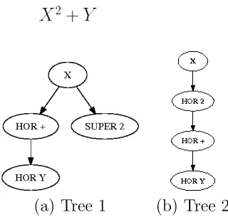
1.2 Two Baseline Structure Trees representing Interpretations of X2+Y . . . . 4
2.1 Two Baseline Structure Trees Representing Interpretations of X2+Y . . . . 14
2.2 Types of Syntactic Parsing . . . 18
2.3 Combination (d) of parse trees for English text (a-c) . . . 19
2.4 Combination of WTNs . . . 20
2.5 GTN for character recognition. [3] . . . 22
3.1 Sigmoid Function . . . 27
3.2 Regions [28] . . . 28
3.3 GTN Math Parser Combination Architecture . . . 31
3.4 Backpropagation in the GTN. Penalties are shown in square brackets . . . . 33
3.5 Threshold and Centroid Table [28] . . . 39
3.6 GTN-Single Penalty Architecture . . . 43
3.7 GTN-Individual Penalties Architecture . . . 44
4.1 Average recognition rates along with standard errors for single-scale experiment 47 4.2 Average recognition rates along with standard errors for two-scales experiment 49 4.3 Segmented bar chart showing Relation and Parent error distribution of 10 runs for 1-Parser GTN structure. Red represents parent error count and blue represents relation error count. Corresponding recognition rate for the run is also shown at the top of each bar . . . 51
4.5 Segmented bar chart showing Relation and Parent error distribution of 10 runs for 3-Parser GTN structure. Red represents parent error count and blue represents relation error count. Corresponding recognition rate for the run is also shown at the top of each bar . . . 52 4.6 Ground Truth BST . . . 52 4.7 DRACULAE Parsed BST . . . 53 4.8 Parent errors comparison between GTN structures having 1, 2 and 3
DRAC-ULAE parsers involved . . . 54 4.9 Relation errors comparison between GTN structures having 1, 2 and 3
Chapter 1
Introduction
Automated mathematical expression recognition is of great practical importance. If technology matures printed document that needs to be converted to electronic form can be done automatically. Recognition of handwritten expressions can be useful with data tablet which can be an alternative and convenient way of writing rather than writing a LATEX expression [28].
[image:13.612.81.461.394.535.2](a) (b)
Figure 1.1: Symbol layout in a textline vs. within a mathematical expression (from Tapia and Rojas [25]). At right the dominant baseline of the handwritten expression is shown in red.
involves two major steps: recognition of individual symbols present in the expression and interpreting the layout of the recognized symbols also known as structural analysis [4]. Structural analysis step may not be so crucial for recognition problems that involve only standard english character 1.1(a). However for problems like recognition of mathematical expressions, the actual position and location of symbols is important and their semantics depends on their arrangement as shown in Figure 1.1(b).
Although there has been number of research that focus on applying different meth-ods of structural analysis [15] [19] [13] [10], every system has improvement limitation in recognition. It has been understood that for most tasks we are faced with a ceiling to the improvement that can be reached with any available machine learning system [27]. [27] explained that the potential loophole of any recognition algorithm is that each of them introduce their own inductive bias to the recognition task and produce different errors. An earlier study on system combination was done by Ali and Pazzani [1] in 1996 who studied the effect of using combining different evidence descriptions of a class on the classification error rate. The result show significant reduction in error rate for half of the different data set used for the experiment and for most of the other set error remains the same.
Thesis Statement: Recognition performance of structural analysis parsers like mathematical recognition parsers can be improved by adopting intelligent parser combina-tion method.
Our combination technique uses Graph Transformer Network(GTN) which was pre-viously used in handwritten character recognition described by LeCun et. al [3]. [3] defined a generalized way in which a series of modules representing key tasks like feature extraction or segmentation in recognition process can be trained. Each module in a Graph Trans-former Network(GTN) takes as input directed graphs and outputs a directed graph, where the graphs have numerical attributes used for learning, and the production of the output is learnt using a gradient descent algorithm. The power of the GTN is that it can combine heterogeneous and dynamic modules and train them using a global optimization criterion, rather than rely upon localized optimization [3].
In GTNs, the produced graphs contain nodes and/or edges that carry numerical attributes, which are used for learning parameters in the GTN (for example, penalties for a relationship defined by edges). During the learning process, labels are used to assign penalties against edges based upon a loss function. These penalties are then backpropagated to adjust weightings in the previous layer of GTN modules. We can see that for labeled graphs that there will be some overlap in their structure to other unlabeled graphs. For example, if our graph is describing the layout of symbols in a mathematical expression such asX2+Y (see Figure 1.2), then we can see that the graph will be similar to that forX+Y
orX2+Y. Using this similarity, we can therefore partially label these additional graphs and
(a) Tree 1 (b) Tree 2
Figure 1.2: Two Baseline Structure Trees representing Interpretations of X2+Y
Chapter 2
Background
Mathematical Expressions MEs form an essential part of scientific and technical documents. Mathematical Expressions can be typeset or handwritten which uses two di-mensional arrangements of symbols to transmit information. Recognizing both forms of mathematical expressions are challenging.
Generally speaking understanding and recognizing mathematical expression, whether typeset or handwritten, involves three activities: Expression localization, symbol recogni-tion and symbol-arrangement analysis. ME localizarecogni-tion involves finding and extracting mathematical expression from the document. Symbol recognition converts the extracted expression image into a set of symbols and symbol arrangement analyzes the spatial ar-rangement of set of symbols to recover the information content of the given mathematical notations.
parallel with latter processes providing contextual feedback for the earlier processes. The order of these recognition activities can vary somewhat, for example, partial identification of spatial and logical relationships can be performed prior to symbol recognition.
2.1
Preprocessing
2.2
Character segmentation
Character segmentation, next step in ME recognition, has long been a critical area of OCR process. Depending upon the requirement, character segmentation techniques is divided into four major headings [21]. Classical approach of segmentation also called dis-section technique consists of partitioning the input image into sub-images based on their inherent features, which are then classified. Another approach to segmentation is a group of techniques that avoids dissection and segments to image either explicitly by classification of pre-specified windows, or implicitly by classification of subsets of spatial features collected from the image as a whole. Another approach is a hybrid approach employing dissection but using classification to select from admissible segmentation possibility. Finally holis-tic approach avoids segmentation process itself and performs recognition entire character strings.
Various techniques have been used for segmentation that involves dissection. White spaces between the characters are used to detect segmentation points. Pitch which is the number of characters per unit of horizontal distance provides a basis for estimating segmen-tation points. The segmensegmen-tation points obtained for a given line should be approximately equally spaced at the distance that corresponds to pitch [21].
Sectioning is done by weighted analysis of horizontal black runs completed versus run still incomplete. Once sectioning determines the regions of segmentation, rules were invoked to segment based on either an increase in bit density or the use of special features designed to detect end-of-character.
In [2], segmentation in cursive handwritten characters is performed in the binary word image by using the contour of the writing. Determination of segmentation regions is done in three steps. In first step a straight line is drawn in the slant angle direction from each local maximum until the top of the word image. While going upward in the slant direction, if any contour pixel is hit, this contour is followed until the slope of the contour changes to the opposite direction. An abrupt change in the slope of the contour indicates an end point. A line is drawn from the maximum to the end point and path continues to go upward in slant direction until the top of the word image. In step 2, a path in the slant direction from each maximum to the lower baseline, is drawn. Step 3 follows the same process as in step 1 in order to determine the path from lower baseline to the bottom of the word image. Combining all the three steps gives the segmentation regions. In [16] segmentation involves detecting ligatures as segmentation points in cursive scripts. Alternatively, concavity features in the upper contour and convexities in the lower contour are used in conjunction with ligatures to reduce the number of potentials segmentation points.
split according to rules based on height and width of the bounding boxes. Intersection of two characters can give rise to special image features and different dissection methods have been developed to detect these features and to use them in splitting a character string images into sub-images.
[9] focuses on segmentation of single and multiple touching character segmentation. [9] proposes a new technique that links the feature points on the foreground and background alternately to get the possible segmentation path. Gaussian mixture probability function is determined and used to rank all the possible segmentation paths. Segmentation paths construction is performed separately for single touching characters and for multiple touching characters. All the paths from to two analysis are collectively processed to remove useless strokes and then mixture Gaussian probability function is applied to decide which on is the best segmentation path.
Different alternative are represented by a directed network whose nodes correspond to the matched subgraphs. Word recognition is done by searching for the path that gives the best interpretation of the word features [9].
2.3
Symbol-Arrangement Analysis
One approach to symbol-arrangement analysis is syntactic approach. Syntactic ap-proach makes use of two dimensional grammar rules to define the correct grouping of math symbols. Co-ordinate grammar for recognition is presented by Anderson. The grammar specifies syntactic rules that subdivide the set of symbols into several subsets, each with its own syntactic subgoal. The final interpretation result is given by the m attribute of the grammar start’s symbol where m represents ASCII encoding of the meaning of symbol-set. Although coordinate grammar provides a clear and well structured recognition approach, its slow parsing speed and difficulty to handle errors are its major drawbacks. In [8], a syntactic approach is adopted in which a system consisting of hierarchy of parsers for the interpretation of 2-D mathematical formulas is described. The ME interpreter consists of two syntactic parser top-down and bottom-up. It starts with a priority operator in the expression to be analyzed and tries to divide it into sub-expressions or operands which are then analyzed in the same way and so on. The bottom-up parser chooses from the starting character and from the neighboring sub-expressions the corresponding rule in the gram-mar. This rule gives instructions to the top-down parser to delimit the zones of neighboring operands and operators.
examination of the symbols to determine the symbol groups and to determine their cat-egories or descriptors. The second pass is parsing or syntax analysis that processes the descriptors synthesized in the first pass to determine the syntactical structure of the expres-sion. A set of predefined rules guides the activities in both the passes.
Another symbol-arrangement analysis approach is recursive projection profile cutting[20]. Cutting by the vertical projection profile is attempted first, followed by horizontal cuts for each resulting regions. The process repeats until no further cutting is possible. The resulting spatial relationships are represented by a tree structure. Although the method looks simple and efficient technique, it is still under study and also involves additional processing for symbols like square root, subscripts and superscripts as these can be handled by projection profile cut.
applies information about the notational conventions of mathematics to remove contra-dictions and resolve ambiguities. The Rank phase uses information about the operator precedence to group symbols into expressions and the Incorporate phase interprets sub-expressions.
Twaakyondo and Okamoto [26] discuss two basic strategies to decide the layout of structure of the given expression. One strategy is to check the local structures of the sub-expressions using a bottom-up method (specific structure processing). It is used to analyze nested structures like subscripts, superscripts and root expressions. The other strategy is to check the global structure of the whole expression by a top-down method (fundamental structure processing). It is used to analyze the horizontal and vertical relations between sub-expressions. The structure of the expression is represented as a tree structure.
Chou in [10] proposed a two-dimensional stochastic context-free grammar for recog-nition of printed mathematical expressions. The recognized symbols are parsed with the grammar in which each production rule has an associated probability. The main task of the process is to find the most probable parse tree for the input expression. The overall probability of a parse tree is computed by multiplying together the probabilities for all the production rules used in a successful parse.
2.4
Baseline Structure Tree
GTN generate BST based on these input. Each node in BST represent the symbol in math-ematical expression and edges represents spatial association between the symbols. Parser also associate a penalty with each of the spatial association.
2.5
DRACULAE Parser
and ordering of operands according to operators.
2.6
Tree Edit Distance
[image:26.612.225.388.184.312.2](a) Tree1 (b) Tree2
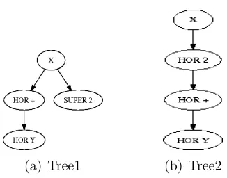
Figure 2.1: Two Baseline Structure Trees Representing Interpretations of X2+Y
Our TED algorithm involves computing the tree edit distance between two Baseline Structure Trees (BST) [28] as shown in Figure 2.1(a) and Figure 2.1(b) representing two interpretations of a mathematical expression having matching symbols but different spatial relationships between them. The expressions are converted into directed trees having nodes with values as a symbol in given expression concatenated with the type of spatial relationship which the symbol has with its parent symbol as shown in Figure 2.1(a) and Figure 2.1(b). Tree edit distance is then given as the number of spatial relationship mismatches between nodes of two trees plus the number of mismatching parents of nodes in two trees. In the given example, Tree2 shows the incorrect interpretation of the expressionX2+Y. The tree
edit distance between Figures 2.1(a) and 2.1(b) is 2. One is due to symbol “2” in Tree2 having a mismatched spatial association with its parent “X” (i.e HOR instead of SUPER as in Tree1) and one due to symbol “+” having mismatching parent (have parent as “2” instead of “X” as in Tree1). Edit distance is then normalized as number of edits / 2n(where n is the number of symbols); 2n is the maximum edit distance, where every symbol has the wrong parent, and in the wrong spatial relationship. Normalization of edit distance is essential in order to meaningfully rank the edits(error) with respect to number of symbols in the expressions that are been compared. To cope with the repeated symbols in the expression symbols needs to be numbered to identify them uniquely.
expression(described in the paper). The edges in the graph represents the relationships between a node in the graph and its ancestor nodes in the symbol layout tree. Given such bipartite graph representations of recognizer output and ground truth, we compute the recognition error by the number of disagreements in terms of stroke labels and spatial relationships which represents distance measure between the two representations.
As there is only one metric involved in evaluating a recognition algorithm from segmentation, classification to structural layout, such a metric can be used to better compare mathematical recognition algorithms as well as provide a single learning function to improve a complete recognition system.
2.7
Parser combination
Classification problem can be solved by having a descriptor for each class which is based on different features taken under consideration and then classifying data to a class based on how close the features of data are to the descriptor of that class. These class-defining descriptors can be formed from a single model or can be formed by combination of mutiple models together called as ensemble of models.
Distribution Summation that involves summation of vectors of all distribution of all satisfied rules from all models and so on [1]. The results shows a statistically significant reduction in error rate for almost all of the data set used or no increase in some cases. For some dataset like wine, the recognition accuracy has increased by factor of 6 from 93.3 percent (with single descriptor) to 98.9 percent (with combined descriptors). This statistically significant reduction in error rate has proven to be true for all the combination techinique tried for the experiment[1].
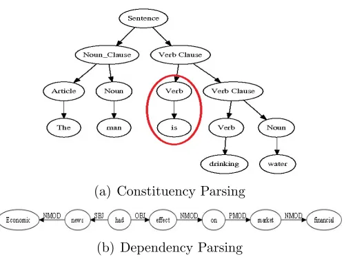
Parser combination involves combining parse trees produced by different parsers, with the goal of reducing error. Parser combination has been explored in a number of areas. Syntactic parsing of a sentence in Natural Language Processing(NLP) can be done in two different ways i.e Constituent Parsing and Dependency Parsing (Figure 2.2). Constituent parsing involves breaking down of sentence into number of syntactic constituents (Noun Clause, Verb Clause or Preposition Clause). Dependency parsing, on the other hand, iden-tify dependencies between words in a sentence and connect the words with that dependency. Our mathematical expression parsing technique is a dependency parsing rather than con-stituency parsing as the technique involves identifying dependencies between symbols in an expression.
Combination of parser can be performed in two different ways as mentioned by Henderson and Brill [17]. The first method is Parse Hybridization in which constituents from each parser’s output are recombined to construct a improved parse. The second is
(a) Constituency Parsing
[image:30.612.183.434.112.300.2](b) Dependency Parsing
Figure 2.2: Types of Syntactic Parsing
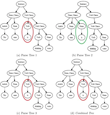
the following Figure 2.3, the constituentVerb is included in two of three parse trees to be combined (tree 1 and tree 3), and so it becomes the part of combined tree. Their experiment showed that these combination techniques gave better recognition results than any of the individual parser used for the experiment. Also the combination technique degrade very less if a poor parser is added to the set.
(a) Parse Tree 1 (b) Parse Tree 2
[image:31.612.74.459.171.574.2](c) Parse Tree 3 (d) Combined Tree
together and finally running a bottom-up parsing algorithm against this chart to obtain maximized well-formed combined parse tree.
Francis Brunet-Manquet in [7] discussed a technique for parser combination for NLP. The combination, however, is applied to dependency parsers unlike the constituent parsers used by Henderson and Brill. The method involves first extracting linguistic data along with confidence rates from a sentence extracted by different syntactic parsers. These linguistic data are then arranged in a respective single structure called dependency structure that identifies the dependencies between these data. From these structures, a common depen-dency structure is obtained consisting of linguistic data contained in different dependepen-dency structures along with different confidence rates associated by different parsers for each data. These confidence rate is nothing but a weighted vote of a parser for a data. Finally a grouping of all linguistic data is done by calculating a combined confidence rate for each data. Combined rate is given as the sum of confidence rates of a data divided by number of parsers that provided this data.
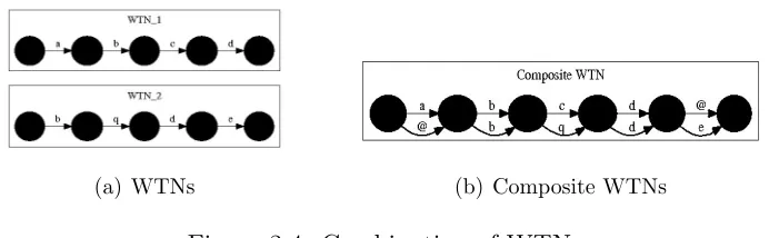
[image:32.612.133.479.454.561.2](a) WTNs (b) Composite WTNs
Figure 2.4: Combination of WTNs
(WTN) are combined using dynamic programming alignment to produce a single WTN. The combination is done sequentially, combining first two and then adding each in turn to the current combined result. The next step is to extract a single WTN from the composite WTN using the voting or scoring scheme that selects the best scoring word sequence from the given hypotheses. One scheme uses frequency of occurrence of particular word type. Higher the frequency, better the score for the word. Other two schemes involve the use of confidence scores generated by ASRs for each word along with frequency scores in voting for best word sequence. One out of the two uses average confidence score while other uses the maximum confidence score for each word type. Experimental results showed that each scoring scheme results in improved word error(WE) reduction than individual ASR system with scheme involving maximum confidence score resulting in maximum WE reduction.
2.8
Graph Transformer Network
[3]. Multiple length sequences which can be best represented in the form of graphs are quite often used for above mentioned tasks. Thus GTN learning can be used for these tasks representing data in the form of graphs in which each path represents a variable length sequence.
Figure 2.5: GTN for character recognition. [3]
Figure 2.5 shows a GTN for recognizing handwritten character string that uses gra-dient based learning.
2.8.0.1 GTN Training
Interpreta-tion graph Gint in which every path represents a interpretation of a segmentation of the
input [a word]. Each arc inGint is associated with a class label and with a penalty for that
class produced by the recognizer.
Another module called the Path Selector takes theGintgraph and the desired labelled
sequence as input and selects paths fromGintthat contains the desired label sequence to give
Constrained graph Gc. Viterbi Transformer then applies Viterbi algorithm to the resulting
graph to select a shortest path (a path with smallest cumulative penalty)Cvit. The loss
function E to minimize is the average penalty of the correct lowest penalty path in the given graph. Gradient based learning is used to train the network. Gradient are computed at different differentiable modules of GTN which are propagated back to so as to compute their gradients and update module parameters.
Partial derivative of the errorEfor the best path with respect to edge penalties on the
Cvit are equal to 1. This is because the loss function is simply the sum of the edge penalties
on Cvit. Since the shortest path is subset of Gc, the partial derivatives of loss function E
with respect to penalties on the arcs of Gc is 1 for those that appear in shortest path and
0 for those that do not. As path selector only selects those paths in Gint that have correct
label sequence, arcs inGint the appear inGc have partial derivatives as 1 or 0, depending on
whether that arc appear in shortest pathGvit. Now these penalties onGintarcs are produced
Chapter 3
Methodology
We describe a novel method of combining syntactic parsers. Our method is based on parse hybirdization techniques presented by Brill and Henderson in [17], in which con-stituents from each parser’s output are recombined to construct a improved parse. Our method made use of GTN which consists of different instances of DRACULAE parsers [28] that produce different BSTs (parse trees). The edges on these parse trees are then penal-ized using penalty function which is described in section 3.1. Penalpenal-ized edges then take part in combination process which is described in section 3.2. After combination, gradients with respect to combination error are computed using the process described in section 3.2.1. Different experiments are performed which is summerized under last section 3.2.2.
3.1
Relationship Penalty Function
Draculae identifies 7 different symbol classes into which different symbols can be classfied. They are as shown in the Table 3.1. Spatial regions around a symbol are partitioned based on the symbol class into seven regions: SU P ER, SU BSC, ABOV E,
BELOW,U P P ER, LOW ER and CON T AIN S.
Table 3.1: Class Membership [28]
Class Symbols
Ascender 0...9, A...Z
Descender g, p, q, y, r, η, ρ
Γ,∆,Θ,Λ,Ξ,Π Open Bracket [{(
Non Scripted Unary binary operators and relation (×,\,≥,÷,≡)
Root √
Variable Range P Q R T S
Center All other symbols
right edges are not included in region definition. Every symbol is reduced to a single point called the centroid of the symbol. A centroid of a symbol lies in exactly one region of its parent symbol.
DRACULAE determines spatial relationships between symbols based on the set of regions for aparent symbol, and the location of the centroid of the associated (child) symbol. Thus a child of a symbol whose symbol class is ascender can lie in either in SU P ER or
SU BSCorABOV E orBELOW orHORregions. For a pair of symbols that are associated in a ground truth baseline structure tree, our model defines a penalty based on how close the centroid of the neighboring symbol is to the vertical boundary (threshold) of these regions. For example, a symbol correctly assigned to the SU P ER region of another symbol will have a penalty based on how close that centroid is to the SU P ER region’s threshold that separates theSU P ER and HOR regions.
Penalties are defined in the interval [0,1], using the sigmoid function:
P(y∆) =
1
1 +e−by∆ (3.1)
where P is the penalty eis constant, b is vertical scaling factor and y∆ is the y-offset of the
Figure 3.1: Sigmoid Function
the steepness of the sigmoid curve. When vertical scaling factor is high, the curve increases steeply which then act more as threshold and when vertical scaling factor is low (closes to zero), the curve flattens.
We describe penalty computation based on types of regions:
3.1.1 Upper and lower regions
Upper regions includeABOV E, U P P ERand SU P ER as shown in Figure 3.2. For upper regions we defined y-offset as,
y∆ = (C−TU)/(Ymax−Ymin) (3.2)
Figure 3.2: Regions [28]
symbol. We normalize the y-offset by dividing offset value by parent symbol’s vertical size. Similarly, for lower regions we defined y-offset as,
y∆= (TL−C)/(Ymax−Ymin) (3.3)
where TL is lower region’s vertical threshold and C is the centroid on neighboring
symbol.
So the penalty function for upper regions becomes:
P(y∆) =
1
Similarly the penalty function for lower regions becomes:
P(y∆) =
1
1 +e−b(C−TL)/(Ymax−Ymin) (3.5)
The upper penalty function (3.4) increases with the increase in y-offset. Whereas the lower penalty function have opposite effect, i.e. the lower penalty function (3.5) decreases with the increase in y-offset. This is described as below:
For upper penalty function:
P = equation
<0.5 if y∆<0
0.5 if y∆= 0
>0.5 if y∆>0
For lower penalty function:
P =
>0.5 if y∆ <0
0.5 if y∆ = 0
<0.5 if y∆ >0
3.1.2 Horizontal Regions
centroid lies below the centre, the offset from lower threshold is uses to compute the penalty value. Let,
Centre= (TU+TL)/2 (3.6)
if C < Centre, centroid lies towards upper vertical threshold, therefore we defined y-offset w.r.t upper threshold as,
y∆ = (TU −C)/(Ymax−Ymin) (3.7)
So the penalty function becomes:
P(y∆) =
1
1 +e−b(TU−C)/(Ymax−Ymin) (3.8)
Whereas. ifC > Centre, centroid lies towards lower vertical threshold, therefore we defined y-offset w.r.t lower threshold as,
y∆= (C−TL)/(Ymax−Ymin) (3.9)
So the penalty function becomes:
P(y∆) =
1
1 +e−b(C−TL)/(Ymax−Ymin) (3.10)
3.2
GTN Architecture
Input to our GTN is a list of mathematical symbols with bounding box co-ordinates. This symbol list is passed to one or more layout parsers. In this first experiment, we have used the publicly available DRACULAE parser [28] 1. DRACULAE parsers have three
Figure 3.3: GTN Math Parser Combination Architecture
parameters, c which controls the vertical position of symbol centroids, ut which defines
the location of upper regions around symbols (e.g. superscript) and lt which defines the
location of lower regions around symbols(e.g subscript) for differentlayout classes assigned to symbols based on their assigned class.
Individual penalties for each edge on different BSTs are computed using the penalty function described in previous section. After the BSTs with edge penalties have been pro-duced, the BSTs are passed to theCombiner module, which has a separate weight for each incoming parser output. The Combiner performs a linear combination of weighted penalties of spatial relationships between two symbols produced by different parsers. This is done by combining all BSTs into a single graph, summing the penalties for any common edges after they have been weighted by their associated connection weightwi, and then applying
0.5∗0.2 + 0.4∗0.6 = 0.34. Since penalty is kept between [0,1], weighted penalty is rounded off to 1 if its greater that 1.0.
The Combiner module output is passed to the BST Scorer module which computes the tree edit distance between the combined BST and ground truth. The set of graph edges
E is partitioned into three disjoint sets: C, the set of correct edges, Ip, the set of edges
with an incorrect parent, and Ir, the set of edges with a correct parent, but an incorrect
relationship. LetN be the total number of edges in the combined BST. We define two edge penalty sums,P
C for the set of correct edges, and
P
Pr the sum of penalties for Ir.
The functionErrord minimized by the GTN is
Errord(C, Ip, Ir) = 1−
(P
Ip+
P
Ir) + (|C| −
P
C)
|C|+|Ip|+|Ir|
= 1− ( P
Ip+
P
Ir) + (|C| −
P
C)
|E|
(3.11)
Errord produces a loss in [0,1]. This function is design for disriminative learning
[3], with the goal of maximimizing penalties on incorrect edges, and minimizing penalties on correct edges.
3.2.1 Learning through Backpropagation
All modules in a GTN must be differentiable with respect to their inputs, allowing error gradients to be backpropagated through each module. The modules in our system include the BST Scorer (a sum module), the Combiner module, and one or more parsers producing graphs with edge penalties in [0,1].
a. Gradients of error at BST Scorer module b. Gradients of error at Linear Combiner
Figure 3.4: Backpropagation in the GTN. Penalties are shown in square brackets penalty for correct and incorrect edges in the combined BST (see Figure 3.4a). Let E be the set of edges with the BST. Therefore partial derivative for Errord w.r.t a penalty on
combined BST edge is given using Equation (2) as follows.
(∂Errord
∂eP
) = ( ∂
∂eP
(1−( P
Ip+PIr) + (|C| −PC)
|E| )) (3.12)
δErrord δeP = 1
|E| if e∈C
− 1
|E| if e∈Ir
− 1
|E| if e∈Ip
The partial derivatives forErrord w.r.t a penalty on a correct edge will be a positive
and partial derivatives for Errord w.r.t a penalty on a incorrect edge will be a negative.
Such a discriminative learning approach minimizes correct edge penalties and also maximizes penalties on incorrect edges, thus reducing the likelihood of selecting incorrect edges in the Combiner module.
containing all incoming edges, from which a minimum penalty spanning tree is computed (see Section 3.2, and Figure 3.4b).
Consider an edge e between symbols X and 2 in the combined BST of Figure 3.4. LeteP be the relationship penalty (0.34). Letw1(0.2) be the input weight to the first parser,
w2(0.7) to the second parser and w3(0.4) to the third parser. Let ep1 (0.5), ep2 (0.5), and
ep3 (0.6) be the penalties on the edges e1, e2 and e3 betweenX and 2 in each of the input
BSTs. For each weight wi, we have:
∂Errord,e ∂wi
= ∂Errord
∂eP
∂eP ∂wi
(3.13) The above equation states that the partial derivative of cumulative error Errord,e
w.r.t a input weightwi is equal to product of partial derivative of cumulative errorErrord,e
w.r.t an edge penalty on combined BST and partial derivative of that same edge penalty w.r.t input weightwi. Here we are just applying the chain rule of computing partial derivatives.
Similarly, for each edge penalty epi in one of the original BSTs we have: ∂Errord,e
∂epi
= ∂Errord
∂eP
∂eP ∂epi
(3.14) The above equation states that the partial derivative of cumulative error Errord,e
w.r.t an edge penalty epi on an input BST is equal to product of partial derivative of
cumulative errorErrord,e w.r.t an edge penalty on combined BST and partial derivative of
that same edge penalty w.r.t edge penaltyepi.
contributed in linear combination to produce penalty for e i.e ifei∈e, then, ∂eP ∂wi =
epi if ei∈e
0 if ei6∈ei
Similarly, ∂eP ∂epi =
wi if ei∈e
0 if ei6∈e
Substituting value of (∂Errord
∂eP ) in equations 3.13 and 3.14, we get,
∂Errord,e ∂wi = 1
|E|
∂eP
∂wi if e∈C
− 1
|E|
∂eP
∂wi if e∈Ir
0 if e∈Ip
∂Errord,e ∂epi = 1
|E|
∂eP
∂epi if e∈C
− 1
|E|
∂eP
∂epi if e∈Ir
0 if e∈Ip
Given the set of such edgesEin the combined BST, the partial derivative of the error w.r.t. wi is is obtained by computing the gradient of error for each edge in the combined
BST as above, and then summing the derivatives:
∂Errord ∂wi
=X
e∈E
∂Errord,e ∂wi
wi(n+ 1) =wi(n)−η∗
∂Errord ∂wi
(3.16) whereη is the learning rate.
In order to compute min at switching surfaces (when edges have same penalty val-ues) we compute penalties using the same penalty functions at a very small higher interval and select minimum of newly computed penalty values. This ensures that we select cor-rect(minimum) penalty function each time there is a tie. We also know that min function is continuous and reasonably regular to achieve convergence using gradient-based learning algorithm [3].
Next we define gradient of Errord,e w.r.t scaling factor (b) of a penalty function.
∂Errord,e ∂b = ∂Errord,e ∂epi ∂epi ∂b (3.17)
From Equation 3.1, we have,
∂epi ∂b =
∂( 1
1+e−by∆)
∂b =
e−by∆
(1 +e−by∆)2
∂(−by∆)
∂b (3.18)
Now depending upon the experimental setup, we have single penalty function for all combining parsers or individual penalty function for each combining parser (described in detail in section 3.2.2).
partial derivatives ofErrord,e w.r.t b. The total gradient w.r.t b will be the sum of all such
partial derivatives computed.
∂Errord
∂b =
X
e∈E
∂Errord,e
∂b (3.19)
However in individual penalty setup, each parser in the setup is associated with individual penalty function. For each edge on a combining BST, we compute the partial derivative of Errord,e w.r.t to that BST’s associated scaling factor bi using equation 3.17.
The total gradient w.r.t scaling factor bi is equal to the sum of all such partial derivatives
computed for all edges of that BST.
∂Errord ∂bi
=X
e∈E
∂Errord,e ∂bi
(3.20) Similarly we compute total gradient of Errord,e w.r.t to scaling factors of other
combining BSTs individually.
The penalty functions’ scaling factor are updated as in the following:
bi(n+ 1) =bi(n)−η∗
∂Errord ∂bi
(3.21) whereη is the learning rate.
The error gradients for each of the parsers need to be computed relative to the parameters defining the vertical locations of SU P ER/HOR, ABOV E/CON T AIN S and
regions (lt), and the vertical position of symbol centroids (c). Both are defined as a per-centage of bounding box height. The partial derivatives of Errord w.r.t region parameters t and care calculated as:
∂Errord,e ∂ut = ∂Errord,e ∂epi ∂epi ∂ut (3.22) ∂Errord,e ∂lt = ∂Errord,e ∂epi ∂epi ∂lt (3.23) ∂Errord,e ∂c = ∂Errord,e ∂epi ∂epi ∂c (3.24)
The relationship penalty epi is based on the proximity of the neighboring (child)
symbol’s centroidC to the region thresholdT and is calculated using equation 3.1 explained in previous section.
From Equation 3.1, we have,
∂epi ∂T =
∂( 1
1+e−by∆)
∂T =
e−by∆
(1 +e−by∆)2
∂(−by∆)
∂T (3.25)
Similarly,
∂epi ∂C =
∂( 1
1+e−by∆)
∂C =
e−by∆
(1 +e−by∆)2
∂(−by∆)
∂C (3.26)
Figure 3.5: Threshold and Centroid Table [28] Again applying chain rule we get:
∂epi ∂ut =
∂epi ∂T
∂T
∂ut (3.27)
∂epi ∂lt =
∂epi ∂T
∂T
∂lt (3.28)
∂epi ∂c =
∂epi ∂C
∂C
∂c (3.29)
Substituting ∂epi ∂ut,
∂epi ∂lt and
∂epi
∂Errord,e
∂ut =
∂Errord,e ∂epi
e−by∆
(1 +e−by∆)2
∂(−by∆)
∂T ∂T ∂ut (3.30) ∂Errord,e ∂lt = ∂Errord,e ∂epi
e−by∆
(1 +e−by∆)2
∂(−by∆)
∂T ∂T ∂lt (3.31) ∂Errord,e ∂c = ∂Errord,e ∂epi
e−by∆
(1 +e−by∆)2
∂(−by∆)
∂C ∂C
∂c (3.32)
We compute ∂Errord ut and
∂Errord
lt by summing the gradient of error for each each edge
penalty in set of edges E as follows,
∂Errord
∂ut =
X
e∈E
∂Errord,e
∂ut (3.33)
∂Errord
∂lt =
X
e∈E
∂Errord,e
∂lt (3.34)
Similarly we compute ∂Errord
c by summing the gradient of error for each each edge
penalty in set of edges E as follows,
∂Errord
∂c =
X
e∈E
∂Errord,e
∂c (3.35)
Each parser’s ut, lt and cparameter values are updated as in the following:
ut(n+ 1) =ut(n)−ρ∗ ∂Errord
lt(n+ 1) =lt(n)−ρ∗ ∂Errord
∂lt (3.37)
c(n+ 1) =c(n)−ρ∗∂Errord
∂c (3.38)
whereρ is the learning rate.
3.2.2 Experiment
Experiments are based on INFTY dataset [23] which consists of ground truth database for characters, words and mathematical expressions. There are 21,056 mathematical expres-sions present in the INFTY dataset which are preprocessed to produce a dataset to be used for our experiment. Experiment consists of dividing the dataset into different sets for GTN training, validation and testing. Experiments are mainly divided into two sections as ex-plained in the following subsections. Each experiments are run multiple times and results are recorded for each run and analyzed.
3.2.2.1 Data Set
• Removing Matrices: DRACULAE expression grammar parses a subset of dialects of mathematics and matrices are not included in the subset. Hence all the expression in the dataset containing matrices are removed in the resulting dataset.
• Removing Malformed: All those expressions that contain more than 1 symbol (more than start symbol) having -1 or null parent, in otherwords if there are more than 1 symbol in an expression having no parent then that expression is to be malformed expression and hence removed the the resulting dataset.
• Removing Single-Symbol: As GTN learning is based on learning relationships between two symbols in an expression, all expressions containing 1 symbol are removed from the resulting dataset as they do not contribute anything in GTN learning process.
• Shuffling: After all the above preprocessing, the expressions are shuffled inorder to randomize expressions in different sets. The order in which data is presented for training is important and its is believed that having randomized data improves the accuracy during training as shuffling enables data to be as far as possible thus making the set statistically unbiased.
Experimental setup is mainly divided into two parts where we try to analyze the effect of having one penalty function for all DRACULAE parsers used in GTN and having individual penalty functions for each DRACULAE parser used in GTN.
Figure 3.6: GTN-Single Penalty Architecture
3.2.2.2 Single Penalty Function Setup
Figure 3.7: GTN-Individual Penalties Architecture
3.2.2.3 Multiple penalty functions Setup
In this setup each BST from DRACULAE parser are penalized with individual penalty function as shown in Figure 3.7. Edge penalties are computed using separate penalty functions and then the resulting BSTs are fed into combiner module for weighted combina-tion of penalized edges. During backpropagacombina-tion learning, gradients computed from a BST’s edges are combined to update the scaling factor of penalty function used to penalized the BST.
3.2.3 Training and testing
number of expressions used in test set 2) total number of incorrectly recognized symbol’s parent (Parent Error) in all the expressions used in test set and 3) total number of incorrectly recognized symbol’s relationship with its parent symbol (Relationship Error).
Chapter 4
Results and Discussion
The results from the experiments described in Chapter 3 are presented in this chap-ter. Section (4.1) presents the experimental results from each individual GTN setup and provides the expression rate along with averages and standard deviations. Section (4.2) provides a distribution of different error types for each GTN setup. Section (4.3) presents a compariative error analysis from different experimental GTN setup for different error types.
4.1
Expression Rate
Following Figures 4.1, 4.2 provide the expression rates from each individual GTN experimental setup which include 1 parser, 2 parsers and 3 parsers. The graphs are bar charts in which each bar represents an expression rate averaged over 10 experimental runs for a given GTN setup. The graphs also show the standard error in terms of a vertical line at the top of each bar. The standard error shows the dispersion of recognition rates around its average for each GTN setup.
4.1.1 Single Penalty Scale
Figure 4.1: Average recognition rates along with standard errors for single-scale experiment learning of both upper and lower thresholds affects the learning of scaling factor.
4.1.2 Discussion
2-parsers GTN structure, which involves combination of 2 DRACULAE parsers in a GTN setup, also achieves a maximum recognition rate of 74% which is higher than plain DRACULAE and have smaller standard error rate as compared to other GTN structures. Smaller the standard error, smaller is the variation from the average and a better represen-tation of recognition result. Thirdly there is 3-parsers GTN setup which achives a maximum recognition rate of 73% and with a standard error in between 1-parser and 2-parsers GTN structures. This graph, overall, shows that with the such a experiment which involves com-bination of parsers we can acheive better recognition rates however results obtained were not as consistent as we desired.
Figure 4.2: Average recognition rates along with standard errors for two-scales experiment increase the penalty of incorrect character sequence as a whole.
Other performance limiting factor can be attibuted to the more deterministic nature of DRACULAE parsers which makes learning harder. DRACULAE consists of multiple heuristic rules that cannot be used in learning especially in gradient based learning.
4.1.3 Upper and Lower Penalty Scales
4.1.4 Discussion
AS can be seen from the graph, the bars looks more or less similar to what we obtained for single scale experimental results. We see lower maximum recognition rate reached with this experiment as compared to single penalty scale experiment. However this experimental results shows lower error rates as compared to single scale experiment as the number of parsers in GTN increases. This means with separate scaling factors we are getting less variation in the recognition rate with increasing number of parsers in GTN which means we are getting a better representation of recognition result.
4.2
Relation and Parent Error
As mentioned in 3.2 section, the recognition error is computed in terms of three disjoint sets from GTN - set of correctly recognized edges, set of edges with an incorrect parent (parent error) and set with edges with a correct parent but an incorrect relationship (relation error). Error function is given at 3.11. Following graphs give the distribution of relation and parent errors from different GTN structures. These graphs provide an overview of how and what distribution of these types of error affect the resulting recognition rate.
4.2.1 Discussion
Figure 4.3: Segmented bar chart showing Relation and Parent error distribution of 10 runs for 1-Parser GTN structure. Red represents parent error count and blue represents relation error count. Corresponding recognition rate for the run is also shown at the top of each bar
[image:63.612.86.526.378.573.2]Figure 4.5: Segmented bar chart showing Relation and Parent error distribution of 10 runs for 3-Parser GTN structure. Red represents parent error count and blue represents relation error count. Corresponding recognition rate for the run is also shown at the top of each bar run. Therefore for different expressions used in the experiment there are more instances of edges in final BST with incorrectly recognized parents than edges with incorrectly recognized relationships with parent. From the graph it is also visible that for the runs with minimum parent and relation errors has better recognition rate. Figures 4.4 and 4.5 similarly shows the error distribution for 10 different runs of 2-parsers and 3-parsers GTN structures re-spectively.These graphs also shows the same behavior in which we have higher parent errors as compared to relation errors. Each of the run showing more parent errors as compared to relation errors can be explained using the following two figures:
Figure 4.7: DRACULAE Parsed BST
Figure 4.6 represents the ground truth BST for one such expression from INFTY dataset and Figure 4.7 represents DRACULAE parsed BST. As can be seens from the figure 4.6 symbol Overline is HOR to symbol Cup and symbols Gamma, Zeta and another Cup are BELOW, SUBSC and HOR to Overline respectively. However in resulting parsed BST (Figure 4.7) we found that symbol Gamma was incorrectly recognized as HOR to symbol Cup which caused Symbols Overline, Zeta and Cup to be incorrectly associated as child symbols of Gamma. This shows a single misrecognition of association between symbols (Cup and Gamma here) leads to 3 parent errors and in our experiments when we obtain a parent error we avoid an additional count of relation error(if there is one) to wrong parent. This is essential to avoid incorrect count of errors. In another term we avoid associating error count of 2 for incorrect parent and relation error just because had the parent was correctly recognized, the relationship with the correct parent could have been correct. As a result we end up having more parent errors than relation errors.
4.3
Error Comparison
error comparison between different GTN structures.
Figure 4.8: Parent errors comparison between GTN structures having 1, 2 and 3 DRACU-LAE parsers involved
4.3.1 Discussion
Figure 4.9: Relation errors comparison between GTN structures having 1, 2 and 3 DRAC-ULAE parsers involved
results and vice-versa.
4.4
Summary
Chapter 5
Conclusion
Thesis Statement: Recognition performance of stuctural analysis parsers like mathematical recognition parsers can be improved by adopting intelligent parser combi-nation method.
We have presented a machine learning algorithm of combining multiple structural recogni-tion algorithms thats supports our hypothesis. Similar experiment was presented by LeCun et. al [3], but it was applied to one dimensional document symbol recognition problem. We showed, in our experiments, that we can combine multiple instances of 2-dimensional math-ematical recognition DRACULAE parsers to obtain a maximum recognition rate of 74% as compared to the best rate of 70% from plain DRACULAE. Our experiment also showed that the total parent and relation errors can be reduced with the combination leading to better recognition of symbol’s parent and its spatial relationship with its parent.
factor in recognition error, therefore we need to employ better handling of parent errors in our experiment to reduce the number of parent errors (may be by highly penalizing parent errors or using an error function that weights parent errors higher) and thus we can obtain better recognition rate than what we obtained from the above experiments.
5.1
Future Work
The performance of our method can be improved by using other performance im-proving machine learning algorithms like Boosting. Most widely used boosting algorithm is AdaBoost (AdaptiveBoosting). AdaBoost train each of the base classifier in sequence using a weighted form of the data set in which weighting coefficient of each data point are adjusted according to the performance of the previous trained classifier so as to give greater weight to misclassified data points. Boosting technique like AdaBoost can be applied to GTN structure to either boost the intermediate results generated by a module of GTN or boost the result given by entire GTN structure.
Bibliography
[1] Kamal M. Ali and Michael J. Pazzani. Error reduction through learning multiple descriptions. Mach. Learn., 24(3):173–202, 1996.
[2] N. Arica and F.T. Yarman-Vural. Optical Character Recognition for Cursive Hand-writing. IEEE Transactions on Pattern Analysis and Machine Intelligence, pages 801–813, 2002.
[3] Y. Bengio, Y. Lecun, L. Bottou, and P Haffner. Gradient-based learning applied to document recognition. Proceedings of the IEEE, 86(11):2278–2324, 1998.
[4] D. Blostein and A. Grbavec. Recognition of Mathematical Notation. Handbook of Character Recognition and Document Image Analysis, pages 557–582, 2001.
[5] Andrew Borthwick, John Sterling, Eugene Agichtein, and Ralph Grishman. Exploiting diverse knowledge sources via maximum entropy in named entity recognition. pages 152–160, 1998.
[6] Eric Brill and Jun Wu. Classifier combination for improved lexical disambiguation. pages 191–195, 1998.
[8] K.F. Chan and D.Y. Yeung. Mathematical expression recognition: a survey. Interna-tional Journal on Document Analysis and Recognition, 3(1):3–15, 2000.
[9] Y.K. Chen and J.F. Wang. Segmentation of Single-or Multiple-Touching Handwritten Numeral String Using Background and Foreground Analysis. IEEE Transactions on Pattern Analysis and Machine Intelligence, pages 1304–1317, 2000.
[10] P. A. Chou. Recognition of equations using a two-dimensional stochastic context-free grammar. In Proceedings of the SPIE Visual Communications and Image Processing IV, 1199:852–863, November 1989.
[11] J. Fiscus. A post-processing system to yield reduced word error rates: Recogniser output voting error reduction (rover). pages 347–352, 1997.
[12] Victoria Fossum and Kevin Knight. Combining constituent parsers. In HLT-NAACL (Short Papers), pages 253–256, 2009.
[13] U. Garain and BB Chaudhuri. Recognition of Online Handwritten Mathematical Ex-pressions. IEEE Transactions on Systems, Man, and Cybernetics, Part B: Cybernetics, 34(6):2366–2376, 2004.
[14] U. Garain and BB Chaudhuri. Recognition of Online Handwritten Mathematical Ex-pressions. IEEE Transactions on Systems, Man, and Cybernetics, Part B: Cybernetics, 34(6):2366–2376, 2004.
[16] K. Gyeonghwan and V Govindraju. A Lexicon Driven Approach to Handwritten Word Recognition for Real-Time Applications. IEEE Transactions on Pattern Analysis and Machine Intelligence, pages 366–379, 1997.
[17] John C Henderson and Eric Brill. Exploiting Diversity in Natural Language Processing: Combining Parsers. Proceedings of the Fourth Conference on Empirical Methods in Natural Language Processing, pages 184–194, 1999.
[18] Zhi-Qiang Liu Jinhai Cai. Integration of Structural and Statistical Information for Unconstrained Handwritten Numeral Recognition. IEEE Transactions on Pattern Analysis and Machine Intelligence, 21(3):263–270, 1999.
[19] Xue-Dong Tian Ming-Hu Ha and Na Li. Structural Analysis of printed mathemat-ical expressions based on combined strategy. Proceedings of the Fifth International Conference on Machine Learning and Cybernetics, Dalian, pages 13–16, 2006.
[20] M Okamoto and B Miao. Recognition of mathematical expressions by using the layout structure of symbols.
[21] Eric Lecolinet Richard G. Casey. A Survey of Methods and Strategies in Character Segmentation. IEEE Transactions on Pattern Analysis and Machine Intelligence, 18(7):690–706, 1996.
[22] Kenji Sagae and Alon Lavie. Parser Combination by Reparsing. Language Technolo-gies Institute. Carnegie Mellon University. Pittsburgh, PA 15213, 2006.
Analysis and Recognition (ICDAR 2005), volume 2, pages 675–679, Seoul, Korea, 2005. IEEE Computer Society Press.
[24] K.C. Tai. The tree-to-tree correction problem. Journal of the association for comput-ing machinery, 26:422–433, 1979.
[25] Ernesto Tapia and Ra´ul Rojas. Recognition of on-line handwritten mathematical expressions using a minimum spanning tree construction and symbol dominance. In
GREC, volume 3088, pages 329–340, 2003.
[26] HM Twaakyondo and M. Okamoto. Structure analysis and recognition of mathematical expressions. In Document Analysis and Recognition, 1995., Proceedings of the Third International Conference on, volume 1, 1995.
[27] Hans Van Halteren, Jakub Zavrel, and Walter Daelemans. Improving data driven wordclass tagging by system combination. pages 491–497, 1998.
[28] Blostein D. Zanibbi, R. and J.R Cordy. Recognizing mathematical expressions using tree transformation. IEEE Transactions on Pattern Analysis and Machine Intelligence, 24(11):1455–1467, 2002.
[29] R. Zanibbi, A. Pillay, H. Mouchere, C. Viard-Gaudin, and D. Blostein. Stroke-based performance metrics for handwritten mathematical expressions. InDocument Analysis and Recognition (ICDAR), 2011 International Conference on, pages 334–338, Sept 2011.
Vita
Amit Arun Pillay was born in Nagpur, Maharashtra, India on September 21, 1984, the son of Arun Pillay and Uma Pillay. He received the Bachelor of Engineering(B.E) de-gree in Information Technology from Veermata Jijabai Technological Institute, Mumbai, India in 2006. He obtained his Master of Science (M.S) degree from Rochester Institute of Technology, United States of America. Currently he is working as a Software Engineer at Silverpop, Atlanta, Georgia, US. His research interest includes Machine Learning, Pat-tern Recognition, Computer Vision and Image Processing. His current research includes combining syntactical pattern recognition techniques.
Permanent address: 615, Shadowood Pkwy SE, Atlanta, Georgia, US
This thesis was typeset with LATEX† by the author.
†LATEX is a document preparation system developed by Leslie Lamport as a special version of Donald
![Figure 1.1: Symbol layout in a textline vs. within a mathematical expression (from Tapiaand Rojas [25])](https://thumb-us.123doks.com/thumbv2/123dok_us/42765.3846/13.612.81.461.394.535/figure-symbol-layout-textline-mathematical-expression-tapiaand-rojas.webp)
![Figure 2.5: GTN for character recognition. [3]](https://thumb-us.123doks.com/thumbv2/123dok_us/42765.3846/34.612.201.409.215.393/figure-gtn-for-character-recognition.webp)
![Table 3.1: Class Membership [28]](https://thumb-us.123doks.com/thumbv2/123dok_us/42765.3846/38.612.231.381.152.245/table-class-membership.webp)

![Figure 3.2: Regions [28]](https://thumb-us.123doks.com/thumbv2/123dok_us/42765.3846/40.612.156.457.119.420/figure-regions.webp)