Knowledge based fundamental and harmonic frequency detection in polyphonic music analysis

Knowledge based Fundamental and Harmonic Frequency

Detection in Polyphonic Music Analysis

Xiaoquan li1_{, Yijun Yan}1_{, Jinchang Ren}1*_, Huimin Zhao2,3_{, S. Zhao}1_{, John Soraghan}1_{, Tariq Durrani}1

1_{Department of Electronic and Electrical Engineering, University of Strathclyde, Glasgow, UK} 2_{School of Computer Science, Guangdong Polytechnic Normal University, Guangzhou, China} 3_{The Guangzhou Key Lab. of Digital Content Processing and Security Technologies,}

China

Abstract. In this paper, we present an efficient approach to detect and tracking the fundamental frequency (F0) from ‘wav’ audio. In general, music F0 and har-monic frequency show the multiple relations; therefore frequency domain analy-sis can be used to track the F0. The model includes the harmonic frequency prob-ability analysis method and useful pre-post processing for multiple instruments. Thus, the proposed system can efficiently transcribe polyphonic music, while taking into account the probability of F0 and harmonic frequency. The experi-mental results demonstrate that the proposed system can successful transcribe polyphonic music, achieved the quite advanced level.

Keywords: Automatic Music Transcription, multiple pitch estimation, poly-phonic music segmentation, fundamental frequency detection.

1

Introduction

In the past decades, detection and tracking of the fundamental frequency (F0) has been an essential part in Blind Signal Separation (BSS) and Music Information Retrieval (MIR) field. Firstly, it is the basic part in semantic level and many features are based on that, for example, if using pitch based features, it would be easier when retrieval since the pitch can be directly used on music. Secondly, pitch tracking can be used on many applications such as humming detection, polyphonic music identification, etc. Thirdly, generally, pitch is an independent direction by contrast with other music re-search directions (timbre, beat, rhythm, chord, melody) that results in pitch can be com-bined with other directions’ methods. At present, F0 tracking can be achieved by using many methods [1] such as probabilistic latent component analysis (PLCA) [2], Non-negative Matrix Factorization (NMF) [3], Support Vector Machines (SVM), Gaussian Mixture Model (GMM), Hidden Markov Model (HMM) [4], etc.

*_{Jinchang. Ren()}

University of Strathclyde, 204 George Street, Glasgow, G1 1XW, United Kingdom

In this paper, we present a tracking F0 frame work which contains five steps: Firstly, we use the Constant Q Translation (CQT) as time-frequency translation function, be-cause CQT is a log frequency representation, which can match with pitch that is also log-frequency representation. Secondly, PLCA can consider the constant harmonic in-terval with log-frequency representations so that small pitch shift or frequency-modu-lated can be detected; another benefit is it can process the different dimensions and can show various features. Thirdly, before doing the harmonic analysis, we should make a smoothing progress. In this step, we use the sigmoid curve and mean filter to remove some relatively small value. Next, we analyses the harmonic structure frame by frame. Finally, we do a post-processing based on several rules.

The rest of the paper is organized as follow: Sect.2 described the related technologies in proposed methods. Sect.3 elaborates the frame work. Experimental results are pre-sented and discussed in Sect.4. Finally, some concluding remarks and future work are summarized in Sect.5.

2

Related work

2.1 Feature Extraction(Front End)

Constant Q Transform (CQT) is a time spectrum transform, and it represents a log-frequency since CQT follows human cochlear structure. What is more, CQT do not stretch spectrum when doing the Fourier transform domain, which is gainful in fre-quency translation [5]. For music analysis, time and log-frefre-quency signal can be con-verted to time and pitch signal because pitch is still log-frequency. The frequency and pitch translate as follows:

pitch = 69 + 12 × log2₄₄₀𝑓 (2.1)

Therefore, pitch is a log-frequency. In addition, all frequencies are scaled by a con-stant factor, which can result in a better frequency resolution in low-frequencies and a better time resolution in high-frequencies.

2.2 Spectrogram factorization

In order to link to the previous step, we use the shift-invariant probabilistic latent com-ponent analysis (SI-PLCA) [6] to do the spectrogram factorization. Because PLCA [7] can improve the resolution in both time and frequency domain at the same time. In addition, the SI-PLCA is useful when the input is a log-frequency presentation. Because the harmonic spacing of all periodic sound is the same. The SI-PLCA can be defined by the following as:

𝑃𝑡(𝑝, 𝑓, 𝑠|𝑤) =_∑ 𝑃(𝑤|𝑠,𝑝,𝑓)𝑃_{𝑃(𝑤|𝑠,𝑝,𝑓)𝑃}𝑡(𝑓|𝑝)𝑃𝑡(𝑠|𝑝)𝑃𝑡(𝑝) 𝑡(𝑓|𝑝)

𝑝,𝑓,𝑠 𝑃𝑡(𝑠|𝑝)𝑃𝑡(𝑝) (2.2)

f∈[1,…,5] where f=3 is the ideal diapason situation when temperament are same and s is the number of instrument sources. 𝑃_𝑡(𝑓|𝑝) is the time-varying log-frequency shifting for pitch p, 𝑃𝑡(𝑠|𝑝) is the source contribution, 𝑃𝑡(𝑝) is the pitch activation, 𝑉𝑤,𝑡 is the log-frequency spectrogram and it is like the 𝑃(𝑤, 𝑡)which is the bivariate probability distribution[8].

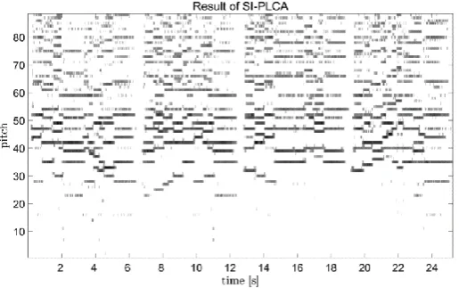
Fig. 1. Result of SI-PLCA with CQT

The Fig.1 is a time-pitch spectrogram, and the value of y axis has been converted from frequency to pitch. It can be seen the signal energy is stronger when pitch is from 30 to 55, because the fundamental frequencies and low order harmonics are concen-trated in this region. On the contrary, the signal energy is weaker in high pitch region due to the dense distribution of high-order harmonics.

3

Proposed method

Fig. 2. Workflow of proposed method

3.1 Mean removal and smoothing

In order to reduce the redundant information, increase the consistency of pitch. A har-monic structure analytics is proposed. In the first step, the result from SI-PLCA will be normalized into [0, 1] by max-mean sigmoid activation function:

y = 1 1+𝑒−𝑧 , 𝑧 =

𝑥−𝑚𝑒𝑎𝑛(𝑥)

max(𝑥)−min (𝑥) (3.1) It adjusts dynamic range. Then, we filter the previous result with mean filter. Further-more, we binaries the filtered result by a fixed threshold 0.5, because sigmoid curve usually set the decision boundary as 0.5. The equation 3.2 is a smoothing in order to avoid high-frequency components because sometimes it might change suddenly large and small. And we define, if there are less than two frame gaps (each frame represents 0.01 sec) between two same notes, then the gap should be filled. And then output [x.*y’] since we need filtered pitch value for the harmonic analysis.

𝑦𝑖= (𝑦𝑖−1+ 𝑦𝑖+ 𝑦𝑖+1)/3 (3.2)

{_𝑦𝑦′′_{= 0. 𝑜𝑡ℎ𝑒𝑟𝑤𝑖𝑠𝑒}= 1, 𝑖𝑓 𝑦 > 0.5 (3.3)

3.2 Harmonic frequency analysis

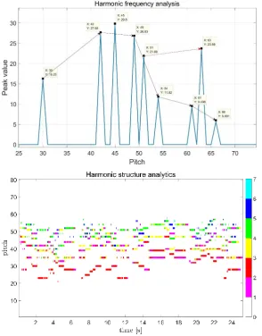
Harmonic frequency analysis is applied in each frame with an interval of 0.01s. The peak values are extracted from SI-PLCA and they would be more if have no smoothing part. The following is the process of this analysis. Firstly, we use the Bayesian model to estimate a rank. The equation has shown below:

𝑃(𝐴|𝐵) =𝑃(𝐵|𝐴)𝑃(𝐴)

𝑃(𝐵) (3.4) where P(A) is harmonic frequency, P(B) is fundamental frequency, P(B|A) is when it is harmonic frequency what the probability to be fundamental frequency, P(A|B) is when it is fundamental frequency, what the probability to be harmonic frequency.

whole frame in order to link them together. Even this database just have four instru-ments, it does not impact the effect. Assuming that we have known the number of in-strument, this approach at least is able to guarantee that one to eight notes play at the same time because the independent value and high probability value would be more.

Fig. 3. The conceptual illustration (top) and the harmonic analysis (bottom)

3.3 Post-processing

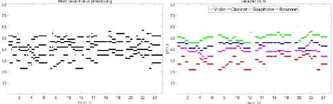
mean value from a length of pitch not just a frame like the last step. We know that generally, the shortest note is 0.08s, so in this part, we filter the notes whose length are smaller than 0.08s. Besides, by training 10% data and testing other 90% data, we get the gain parameter (1.1*instruments) as the standard value to compare with the rank. First of all, we fill up the vacant when it is below 0.08s, but set the rank as the top one such as 6. Secondly, we made a comparison with mean rank value and gain parameter. If the mean value of each rank higher than the gain parameter, this pitch will be con-sidered as foreground and background otherwise. The gain parameter comparison would show on the result.

Fig. 4. Result from post-processing (left) and Ground truth with four instrument sources (right)

4

Experimental results

4.1 Experiment setup

To evaluate the performance of our method, we present our method on BACH10 dataset [9] which contains ten quartets of four part polyphonic pieces with length range from 27 to 45 seconds. Four instrument sources such as violin, clarinet, saxophone, and bas-soon are included. And we also use three widely used evaluation criteria to present the performance of proposed method.

Precision = ∑ 𝑇𝑃(𝑡) 𝑇 𝑡=1 ∑𝑇 𝑇𝑃(𝑡)+𝐹𝑃(𝑡)

𝑡=1 , Recall =

∑𝑇_𝑡=1𝑇𝑃(𝑡) ∑𝑇 𝑇𝑃(𝑡)+𝐹𝑁(𝑡)

𝑡=1 (4.1)

F − measure =2×𝑝𝑟𝑒𝑐𝑖𝑠𝑖𝑜𝑛×𝑟𝑎𝑐𝑎𝑙𝑙

𝑝𝑟𝑒𝑐𝑖𝑠𝑖𝑜𝑛+𝑟𝑎𝑐𝑎𝑙𝑙 (4.2)

where TP is the number of correct non-zero F0 values, FP is the number of incorrect non-zero F0 values, and FN is the number of incorrect zero or non-zero F0 values. The time step of each frame in both test result and ground truth is 0.01s. In addition, F-measure [1] is defined as the F0 mean of precision and recall, if the two values are closer, the F-measure would be higher.

4.2 Evaluation Results and Discussion

used to calculate the mean pitch value. In Table 1, the gain parameter illustrates what is the best gain parameter in this database. We can see that the best one is 4.4 when there are four instruments. And when the gain parameter is lower, the precision and recall would be closer. What is more, even the database is only four instruments; the gain parameter must higher than the number of the instruments.

The system configuration (Table 2) is using 4.4 as the gain parameter, it demon-strates every part of the system is indispensable, where A is CQT and SI-PLCA, B is smoothing, C is harmonic structure analysis, and D is post-processing. We can see that each module has its contribution and every module is indispensable. Part A mainly transform the one-dimensional to both time and frequency domain. Meanwhile, they emphasize the energy in lower frequency. Table 2 shows that the highest recall and lowest precision are both A. That means part A include a high similarity. When B has been added after A, the recall value decreases slightly. Because the points removed by part B do not impact the recall. Part C is the most critical part due to increasing almost 30%. The smoothing (B) and post-processing (D) part both occupy the same important degree. When both module B and D are integrated with A and C together, the system would show the highest F-measure. In addition, when F-measure is higher, precision and recall are closer, and our system configuration demonstrates the effective results.

5

Conclusion

In this paper, we proposed a framework to track the fundamental frequency in poly-phonic music pieces even performed by different instruments. By estimating the har-monic probability analysis followed by CQT and SI-PLCA, the fundamental frequency (F0) can be successfully detected with bio-inspired rule-based post-processing. In fu-ture work, we will extend more datasets to testify this framework such as MAPS [10] and RWC [11]. We will also apply a deep learning based method to detect how many notes per frame. If this step is achieved well, it can not only find how many notes per frame, but also information about which instruments they come from. In addition, there still exist other modules such as beat and chord based methods [12] [13], which can be extended as future study, where denoising and spectrum analysis will be highlighted even for broadcasting applications [14-16].

Table 1. Different gain parameter

Gain

Parameter Precision Recall F- measure

4.2 79.99 83.31 81.62

4.3 79.56 84.90 82.14

4.4 79.35 86.73 82.88

4.5 78.63 86.58 82.41

4.6 78.23 87.03 82.39

Table 2. System configuration

System

configuration Precision Recall F- measure

A 33.39 93.62 49.22

A+B 35.6 93.09 51.50

A+B+C 74.54 83.91 78.95

A+C+D 72.74 85.84 78.75

6

Acknowledgement

This work was supported by the National Natural Science Foundation of China (61672008), Guangdong Provincial Application-oriented Technical Research and De-velopment Special fund project (2016B010127006, 2015B010131017), the Natural Science Foundation of Guangdong Province (2016A030311013,2015A030313672), and International Scientific and Technological Cooperation Projects of Education De-partment of Guangdong Province (2015KGJHZ021).

Reference

1. Bay, M., Ehmann, A. F., & Downie, J. S. (2009, October). Evaluation of Multiple-F0 Esti-mation and Tracking Systems. InISMIR(pp. 315-320).

2. Arora, V., & Behera, L. (2015). Multiple F0 estimation and source clustering of polyphonic music audio using PLCA and HMRFs.IEEE/ACM Transactions on Audio, Speech and Lan-guage Processing (TASLP),23(2), 278-287.

3. Cogliati, A., Duan, Z., & Wohlberg, B. (2017). Piano Transcription With Convolutional Sparse Lateral Inhibition.IEEE Signal Processing Letters,24(4), 392-396.

4. Su, L., & Yang, Y. H. (2015). Combining spectral and temporal representations for mul-tipitch estimation of polyphonic music.IEEE/ACM TASLP,23(10), 1600-1612.

5. Schörkhuber, C., & Klapuri, A. (2010, July). Constant-Q transform toolbox for music pro-cessing. In7th Sound and Music Computing Conference, Barcelona, Spain(pp. 3-64). 6. Benetos, E., Cherla, S., & Weyde, T. (2013). An efficient shift-invariant model for

poly-phonic music transcription. In6th Int. Workshop on Machine Learning and Music. 7. Smaragdis, P., Raj, B., & Shashanka, M. (2006). A probabilistic latent variable model for

acoustic modeling.Advances in models for acoustic processing, NIPS,148, 8-1.

8. Benetos, E., & Dixon, S. (2013). Multiple-instrument polyphonic music transcription using a temporally constrained shift-invariant model.The Journal of the Acoustical Society of America,133(3), 1727-1741.

9. Duan, Z., Pardo, B., & Zhang, C. (2010). Multiple fundamental frequency estimation by modeling spectral peaks and non-peak regions.IEEE Transactions on Audio, Speech, and Language Processing,18(8), 2121-2133.

10. Emiya, V., Bertin, N., David, B., & Badeau, R. (2010). MAPS-A piano database for mul-tipitch estimation and automatic transcription of music.

11. Goto, M., Hashiguchi, H., Nishimura, T., & Oka, R. (2002, October). RWC Music Database: Popular, Classical and Jazz Music Databases. InISMIR(Vol. 2, pp. 287-288).

12. Grosche, P., & Muller, M. (2011). Extracting predominant local pulse information from mu-sic recordings.IEEE Trans. Audio, Speech & Language Processing,19(6), 1688-1701. 13. Müller, M., & Ewert, S. (2011). Chroma Toolbox: MATLAB implementations for extracting

variants of chroma-based audio features. InProc. of the 12th _{Int. Conf. on Music Information}

Retrieval (ISMIR), 2011.

14. Ren, J. and Vlachos, T. (2007), Efficient detection of temporally impulsive dirt impairments in archived films, Signal Processing, 87(3): 541-551

15. Ren, J., Jiang, J., et al (2010), Fusion of intensity and inter-component chromatic difference for effective and roust colour edge detection, IET Image Processing, 4(4); 294-301. 16. Jiang, J., et al (2011), Live: An integrated production and feedback system for intelligent