City, University of London Institutional Repository
Citation:
Najibi, F., Alonso, E. ORCID: 0000-0002-3306-695X and Apostolopoulou, D.
ORCID: 0000-0002-9012-9910 (2018). Optimal Dispatch of Pumped Storage Hydro
Cascade under Uncertainty. In: 2018 UKACC 12th International Conference on Control
(CONTROL). (pp. 187-192). IEEE. ISBN 978-1-5386-2864-5
This is the accepted version of the paper.
This version of the publication may differ from the final published
version.
Permanent repository link:
http://openaccess.city.ac.uk/20142/
Link to published version:
Copyright and reuse: City Research Online aims to make research
outputs of City, University of London available to a wider audience.
Copyright and Moral Rights remain with the author(s) and/or copyright
holders. URLs from City Research Online may be freely distributed and
linked to.
Optimal Dispatch of Pumped Storage Hydro
Cascade under Uncertainty
Fatemeh Najibi, Eduardo Alonso, Dimitra Apostolopoulou
City, University of London
London, UK, EC1V 0HB
Email:
{Fatemeh.Najibi, E.Alonso, Dimitra.Apostolopoulou}@city.ac.uk
Abstract—In this paper, we propose an optimal dispatch scheme for a pumped storage hydro cascade that maximizes the energy per cubic meter of water in the system taking into account uncertainty in the net load variations. To this end, we introduce a model to describe the behaviour of a pumped storage hydro cascade and formulate its optimal dispatch. We then incorporate forecast scenarios in the optimal dispatch, and define a robust variant of the developed system. The resulting optimization problem is intractable due to the infinite number of constraints. Using tools from robust optimization, we reformulate the resulting problem in a tractable form that is amenable to existing numerical tools and show that the computed dispatch is immunised against uncertainty. The efficacy of the proposed approach is demonstrated by means of a realistic case study based on the Seven Forks system located in Kenya.
Index Terms—Robust optimization, Hydroelectric system, Pumped storage hydro cascade, Optimal Dispatch Scheme.
I. INTRODUCTION
Renewable-based resources have been integrated into power systems at a very high pace the last decades making the reliable operation of power systems more challenging. Due to the inherent variable and intermittent nature of renewable resources adequate generation from traditional resources needs to be scheduled to ensure the load generation balance and the secure operation of power systems. One way to make the integration of renewable resources to the grid more smooth is to better utilize existing system resources, e.g., through coupling of resources that have complimentary characteristics. Such candidates are hydro and solar resources in the sense that when the power output of one, e.g., solar generation is high, the potential power output of the other is lower, e.g., hydro generation (e.g. [1], [2]). This is true when the sun irradiance is high and there is no rainfall thus reducing the water inflows to the hydroelectric system and the potential output of the hydroelectric resource. Besides the complementarity effect pumped hydro and solar resources are nicely combined together because the first may serve as a “storage” device for the latter. When the solar generation exceeds the net load then the remaining power may be used to move water upstream in the pumped hydroelectric power system. Moreover, when the solar generation is not sufficient to meet the net load the pumped hydro has satisfactory ramping capabilities to quickly ramp up to meet the load.
In order to integrate solar generation with hydro resources and maximize their benefits mathematical models and algo-rithms that are able to effectively deal with the uncertainty need to be developed. In [3], dynamic programming is used to determine hydroelectric power scheduling. The authors in [4] use Monte Carlo techniques for the short-term operation of the Itaipu hydroelectric power system subject to inflow
uncertainties. Another case study is presented in [5] where a model predictive control scheme for the Mid-Columbia hydropower system is proposed.
In this work: i) We develop a deterministic model for the operation of a pumped storage hydro cascade, ii) We incorporate forecast scenarios in an optimization and define a robust variant of the developed pumped storage hydro cascade system. Using tools from robust optimization we reformulate the resulting problem in a tractable form that is amenable to existing numerical tools, while offering immunization of the computed dispatch against uncertainty, iii) We demonstrate the proposed approach through a realistic system based on the Seven Forks system located in Kenya.
II. HYDROELECTRIC SYSTEM MODEL
In this section, we introduce the hydropower function, the pumped storage hydro modelling and the scheduling con-straints that are utilised to develop our framework.
We consider a hydroelectric power system with N hydro-electric power plants indexed by N = {1, . . . , N} that we wish to schedule for a time period T = {1, . . . , T}. Let us assume thatKplants are pumped storage hydro and comprise the set K ={1,2, . . . , K}, and the remaining plants are in
˜
N =N \K. We model the behavior of the system in discrete time which is a valid assumption since we consider the steady state operation of the hydroelectric system (e.g. [6], [7]).
A. Hydroelectric Power Output
A hydroelectric power planti∈N˜ output is a function of the water discharge and the head level of the plant. The head is the difference between the level of the reservoir and the tail water. In particular, the power of a hydroelectric power plant
i at timetis defined as
Pi(t) =ηiρ g hi(t)qi(t),∀i∈N˜, ∀t∈T, (1)
where ρ is the density of the water in kg/m3; g is the gravitational acceleration in m/s2; hi(t) is the net head of
water of hydropower plant i at time t in m; qi(t) is the
discharge of water of plant iduring time tin m3/s;ηi is the
efficiency of the turbine generator.
The dispatch of a hydroelectric power system is usually formulated as an optimization problem. The use of (1) as a constraint in the dispatch algorithm makes the optimization problem non-convex since it is a non-linear constraint. Thus, several works are dedicated into determining approximations of (1) (e.g., [5]). A linear function fit to the three-dimensional hydropower production function denoted by
˜
is a good approximation of (1) as shown in [8].
The power output of each hydroelectric power planti∈N˜
is constrained by a minimum and a maximum output, i.e.,
Pim≤P˜i(t)≤PiM, for allt∈T. Similar statements are true
for the head levels and the water discharge rates. Thus, we have that
Pim≤P˜i(t)≤PM
i ,∀i∈N˜,∀t∈T, (3) hmi ≤hi(t)≤hMi ,∀i∈N˜,∀t∈T, (4) qim≤qi(t)≤qMi ,∀i∈N˜,∀t∈T. (5)
B. Cascading Effect of Hydroelectric System
The cascading effect of a hydroelectric system refers to the water balance between reservoirs. In other words the water at a downstream dam is affected by the discharge and spillage at upstream dams, and inflows. In the inflow parameters, evaporation and percolation losses are taken into account. Furthermore, in the water balance equation the time that the water needs to travel from one dam to the other should be considered.
A mathematical formulation of the water balance of the hydroelectric power system may be expressed as
V1(t) = V1(t−1) + (r1(t)−q1(t)−s1(t))∆t, (6)
V2(t) = V2(t−1) + (r2(t) +q1(t−τ1) +s1(t−τ1)
−q2(t)−s2(t))∆t, (7)
.. .
VN(t) = VN(t−1) + (rN−1(t) +qN−1(t−τN−1)
+sN−1(t−τN−1)−qN(t)−sN(t))∆t, (8)
where Vi(t) is the live volume of hydroelectric power plant i at the end of time t in m3; τi is the time delay between
reservoiriandi+ 1, i.e., the time water needs to travel from one to the other ;ri(t)is the inflow into hydroelectric power
plant i during time to t ; si(t) is the spillage discharge of
hydroelectric power planti during time tot; and∆t the time interval between the decision making, e.g., one hour.
There are constraints associated with the reservoir storage volume limits of each hydroelectric power planti∈N, which are defined as
Vm
i ≤Vi(t)≤ViM,∀i∈N , t∈T. (9)
C. Pumped storage hydro modelling
Pumped storage hydroelectric plants are designed to serve the peak load at certain times, e.g., peak hours, with hy-droelectric energy and then pumping the water back up into the reservoir at other times, e.g., light load periods. Thus, two intervals need to be considered when modelling the operation of pumped storage hydroelectric systems: intervals of generation and intervals of pumping. In any one interval, the plant can be (i) pumping or (ii) generating. The idle case may be presented as either pump or generate .
Let us assume that hydro electric plantkin the cascade is a pumped storage hydro plant. Then, for the generation intervals
t we have:
˜
Pqk(t) = αk+βkhk(t) +γkqk(t), (10)
Vk(t) = Vk(t−1) + (rk(t) +qk−1(t−τk−1)
+sk−1(t−τk−1)−qk(t)−sk(t))∆t, (11)
where P˜qk(t) is the power output of pumped storage hydro plant kat timet.
For the pump intervalst0 we have:
˜
Pwk(t
0) = −α
k−βkhk(t0)−γkwk(t0), (12) Vk(t0) = Vk(t0−1) + (rk(t0) +qk−1(t0−τk−1)
+sk−1(t0−τk−1) +wk(t0)
−sk(t0))∆t0, (13)
where P˜wk(t
0) is the power needed to pump the water of
pumped storage hydro plant k at time t0 and w
k(t0) is the
pumping rate at timet0.
We represent the intertemporal water balance constraints that relate the charge/discharge decisions, combining (11) and (13) with
Vk(t) = Vk(t−1) + (rk(t) +qk−1(t−τk−1)
+sk−1(t−τk−1) +wk(t)−qk(t)
−sk(t))∆t, (14)
These equalities serve to ensure that the reservoir accumulates water during the light load conditions so as to discharge water in subsequent peak load hours. The constraints associated with the ranges with discharge and pumping rates are
uqk(t)P
m qk ≤
˜
Pqk(t)≤uqk(t)P
M
qk,∀k∈K, t∈T, (15)
uqk(t)q
m
k ≤qk(t)≤uqk(t)q
M
k ,∀k∈K, t∈T, (16) uwk(t)P
m wk ≤
˜
Pwk(t)≤uwk(t)P
M
wk,∀k∈K, t∈T,(17)
uwk(t)w
m
k ≤wk(t)≤uwk(t)w
M
k ,∀k∈K, t∈T. (18)
Note that the minimum and maximum discharge (pumping) rates are both multiplied by the operational state status vari-able uqk(t) (uwk(t)). Whenever the pumped storage hydro generates (pumps) at time t, the associated status variable
uwk(t) (uqk(t)) is 0, resulting in the pumping output wk(t) (discharge output qk(t)) being 0. This formulation preserves
the linearity of the constraints, which helps with the compu-tational tractability. Furthermore, in order to ensure that the pumped storage hydro does not both pump and generate at the same twe include (e.g., [9])
0≤uqk(t) +uwk(t)≤1,∀t∈T, (19)
uqk(t), uwk(t)∈ {0,1},∀t∈T. (20) D. Reservoir geometry
There is a relationship that connects the volume of a reservoir at time t, i.e., Vi(t) with a certain head level, i.e., hi(t). This mapping may be approximated by a linear
func-tion when referring to short-term operafunc-tion of hydroelectric systems since for small head level differences we have small volume differences. We denote this relationship by
hi(t) =ζ1Vi(t) +ζ2,∀i∈N , t∈T, (21)
whereζ1,ζ2 some coefficients.
III. OPTIMAL DISPATCH OF PUMPED STORAGE HYDRO CASCADE
A. Power Balance Constraint
The output of a hydroelectric power system is used to meet the net load at every time instant t ∈T. In this regard, we have
X
i∈N˜
˜
Pi(t)+
X
k∈K
( ˜Pqk(t)−P˜wk(t)) = ∆PL(t),∀t∈T, (22)
where∆PL(t)is the net load at time t. We use the net load
definition since we wish to include in our formulation the effects of renewable resources.
B. Objective Function Formulation
When formulating the optimal dispatch of a pumped storage hydro cascade we wish to maximise the energy per cubic meter of water in the system, i.e., system efficiency. To this end, we wish to operate each dam at the highest possible head and minimise the spillage effects [10]. The rationale behind this statement is that for the same discharge rate of waterq for a higher head level, i.e., h1 > h2, the power output is higher,
i.e.,P1> P2, as it may be easily seen through (1).
In this regard, we wish to maximise the head of each reser-voir at every time instant, i.e., hi(t), for alli ∈ N, t ∈T.
We have
X
t∈T X
i∈N
hi(t). (23)
The spilling of water may be seen as the discharge of a water amount without any power generation. In this regard, water spilled is water that is not used by the hydroelectric power system. So we wish to minimize spillage effects:
MP
t∈T Pi∈N si(t). We have:
M X
t∈T X
i∈N
si(t), (24)
withM a large positive constant.
C. Optimal Dispatch Formulation
In the previous sections, we have identified the objective function and the constraints that will be included in the optimal dispatch formulation of the pumped storage hydro cascade. In this regard, we use (23) and (24) to construct the objective function. The decision variables of the optimal dispatch are the live volumesVi(t); the head levelshi(t); the spillagesi(t);
and the water discharge ratesqi(t), for alli∈N andt∈T,
the pumping rates of the pumped storage hydro units wk(t),
the operational state status variables uqk(t) (uwk(t)) for k ∈
K and t ∈ T. Once, the head level and water discharge rate of each dam are determined we may calculate the power output using (2) and (10). The power needed to pump may be calculated using (12). The power balance constraint now becomes:
P
i∈N(αi+βihi(t) +γiqi(t))
−P
k∈K(αk+βkhk(t) +γkwk(t)) = ∆PL(t),∀t∈T.(25)
We represent the cascading constraints by (6)-(8) and (14) for the hydroelectric plants and the pumped storage hydro plants, respectively; the relationship between the head level and live volume by (21); the power balance by (25). The lower and upper bounds of decision variables are included through
(4)-(5), and (9). The power output limits constraints in (3) are now
Pim≤αi+βihi(t) +γiqi(t)≤PiM,∀i∈N˜, t∈T. (26)
Moreover, (15), (17) are rewritten as:
uqk(t)P
m
qk ≤αk+βkhk(t) +γkqk(t)≤uqk(t)P
M qk,
∀k∈K, t∈T. (27)
uwk(t)P
m
wk≤αk+βkhk(t) +γkwk(t)≤uwk(t)P
M wk,
∀k∈K, t∈T. (28) Note that the constraints for the discharge and pumping rates in a pumped storage hydro plant are taken into account through (16), (18). The constraints that ensure that the pumped storage hydro does not both pump and generate are (19), (20).
max
hi(t),si(t),qi(t),wk(t),
uqk(t),uwk(t),Vi(t) X
t∈T X
i∈N
hi(t)−M
X
t∈T X
i∈N
si(t)
subject to(4)−(9),(14),(16),(18)−(21),
(25)−(28). (29)
The resulting optimization problem given in (29) is a mixed-integer linear program (MILP) due to the presence of the binary variables uqk(t), uwk(t), for all k ∈ K, t ∈ T. The output of (29) determines the head levels, power output, volume, spillage and water discharge for every hydroelectric power plant at every time instant in the period of interest. It also determines the pumping and generating intervals, pumping rates, and the power needed for pumping for the pumped storage hydro at every time instant in the period of interest.
IV. ROBUST OPTIMAL DISPATCH
The optimal dispatch of the pumped storage hydro cascade is used for the short term operation of a hydroelectric power system. However, the net load is usually a forecast of the actual net load and thus, contains some forecast error. This situation is exacerbated when the hydroelectric power system is coupled with some renewable resource, such as solar generation, which is intermittent and variable. In this regard, it is useful to make the optimal dispatch robust to uncertainty. In this section, we introduce uncertainty into the net load and perform a stochastic analysis, taking forecast errors into account. The resulting optimization problem is intractable; thus, we recast it into a tractable form that is immune to uncertainty. In a similar manner uncertainty in time delays or inflows to the system could be taken into account.
A. Uncertainty Modelling
We model the net load∆PL with two components: (i) the
nominal prediction, i.e.,∆PL; and (ii) a random forecast error
vector δ = [δ(1), . . . , δ(T)]> ∈ ∆t ⊂ RT. Thus we have:
∆PL = ∆PL+δ. We use the vectorδto construct bounds of
the forecast error, which are modelled as follows:
withθ(t)>0,∀t ∈ T. The power balance constraint given in (25) may now be written as
P
i∈N(αi+βihi(t) +γiqi(t))
−P
k∈K(αk+βkhk(t) +γkwk(t))
= ∆PL(t) +δ(t),∀δ(t)∈∆t, t∈T. (31)
However, (31) has to be met for every δ(t); thus making it infeasible. In order to make the problem feasible we express the uncertainty in the inequality constraints. To this end, we introduce piecewise affine control rules as presented in [11]. We now define the decision variable of the water discharge of every hydroelectric power planti∈N (pumping rate of the pumped storage hydro plantsk∈K) at timetto consist of a deterministic component qd
i(t) (wkd(t)) and another term that
depends on the uncertain error:
qi(t) =qdi(t) +aqi(t)δ(t),∀i∈N , δ(t)∈∆t,∀t∈T, (32)
wk(t) =wdk(t) +awk(t)δ(t),∀k∈K, δ(t)∈∆t,∀t∈T,(33) where
X
i∈N
aqi(t)− X
k∈
awi(t) = 1,∀t∈T. (34) The stochastic terms imply that if an uncertain error is realized, it is allocated to the water discharge rates, and pumping rates (if pumped storage hydro is at a pumping interval) of hydroelectric power plants according to the coefficientsaqi(t) andawk(t), adjusting their set-pointsq
d i(t),w
d k(t).
Based on this formulation (31) now becomes
P
i∈N(αi+βihi(t) +γiqdi(t))
−P
k∈K(αk+βkhk(t) +γkwdk(t))
= ∆PL(t), t∈T, (35)
i.e., we moved the uncertainty from the equality constraint to the inequality constraints. In particular, the uncertainty sources are introduced in the inequality constraints that include qi(t)
and wk(t). However, moving the uncertainty to qi(t) and wk(t) has as a result to express the spillage effects in terms
of piecewise affine control rules due to (6)-(8), (14). In this regard, we have
si(t) =sdi(t) +asi(t)δ(t),∀i∈N, δ(t)∈∆t, t∈T,(36)
aqi(t) +asi(t) = 1,∀i∈N˜, t∈T, (37)
aqk(t) +ask(t)−awk(t) = 1,∀k∈K, t∈T. (38) Now, (6)-(8), (14) become
V1(t) = V1(t−1) + (r1(t)−qd1(t)−s
d
1(t))∆t, (39)
V2(t) = V2(t−1) + (r2(t) +qd1(t−τ1) +sd1(t−τ1)
−qd2(t)−sd2(t))∆t, (40) ..
.
VN(t) = VN(t−1) + (rN−1(t) +qNd−1(t−τN−1)
+sdN−1(t−τN−1)−qdN(t)−s d
N(t))∆t, (41)
and
Vk(t) = Vk(t−1) + (rk(t) +qkd−1(t−τk−1)
+sdk−1(t−τk−1) +wkd(t)−q d k(t)
−sdk(t))∆t. (42)
We also have the constraints for the additional decision vari-ables
−1≤aqi(t)≤1,∀i∈N˜, t∈T, (43)
−1≤asi(t)≤1,∀i∈N, t∈T, (44)
−uqk(t)≤aqk(t)≤uqk(t),∀k∈K, t∈T, (45)
−uwk(t)≤awk(t)≤uwk(t),∀k∈K, t∈T. (46) We include (45) and (46) to ensure that aqk(t)(awk(t)) will be zero when the pumped storage hydro plant is at a pumping (generating) mode.
The stochastic optimization problem may now be written as
max
hi(t),si(t),qi(t),wk(t),
aqi(t),asi(t),awk(t), uqk(t),uwk(t),Vi(t)
X
t∈T X
i∈N
hi(t)−M
X
t∈T X
i∈N
si(t)
subject to(4),(9),(19)−(21),(34),(35),(37)−(46), qim≤qid(t) +aqi(t)δ(t)≤q
M i ,
∀i∈N˜, δ(t)∈∆t, t∈T
Pim≤αi+βihi(t) +γi(qdi(t) +aqi(t)δ(t))
≤PiM,∀i∈N˜, δ(t)∈∆t, t∈T. uqk(t)P
m
qk ≤αk+βkhk(t) +γk(q
d k(t)
+aqk(t)δ(t))≤uqk(t)P
M
qk,∀k∈K,
δ(t)∈∆t, t∈T uwk(t)P
m
wk ≤αk+βkhk(t) +γk(w
d k(t)
+awk(t)δ(t))≤uwk(t)P
M
wk,∀k∈K,
δ(t)∈∆t, t∈T uqk(t)q
m
k ≤qkd(t) +aqk(t)δ(t)
≤uqk(t)q
M
k ,∀k∈K, δ(t)∈∆t, t∈T, uwk(t)w
m k ≤w
d
k(t) +awk(t)δ(t)
≤uwk(t)w
M
k ,∀k∈K, δ(t)∈∆t, t∈T.
(47)
B. Equivalent Tractable Reformulation
The optimization problem given in (47) cannot be solved directly because some constraints apply for all δ(t)∈∆t, t∈
T; thus, the intersection of an infinite number of constraints. In this regard, we recast (47) into a tractable problem [12]. To make this reformulation more clear, we first go through a simple inequality constraint, i.e., qm
i ≤qid(t) +aqi(t)δ(t)≤
qM
i and follow this procedure for all of the constraints that
contain δ(t). For the upper bound, we have that:
qd
i(t) +aqi(t)δ(t)≤q
M i
(30)
⇔
qd
i(t) +|aqi(t)|θ(t)∆PL(t)≤q
M i ⇔
−qMi −q d i(t)
θ(t)∆PL(t)
≤aqi(t)≤
qMi −qdi(t)
θ(t)∆PL(t)
. (48)
In the same vein, for the lower bound we have that:
qdi(t) +aqi(t)δ(t)≥q
m i
(30)
⇔
qid(t)− |aqi(t)|θ(t)∆PL(t)≥q
m i ⇔
− qid(t)−qmi
θ(t)∆PL(t) ≤aqi(t)≤
qd i(t)−qmi
The resulting tractable mixed integer linear programming may be written as:
max
hi(t),si(t),qi(t),wk(t),
aqi(t),asi(t),awk(t), uqk(t),uwk(t),Vi(t)
X
t∈T X
i∈N
hi(t)−M
X
t∈T X
i∈N
si(t)
subject to(4),(9),(19)−(21),(34),(35),(37)−(46)
qmi ≤qdi(t)− |aqi(t)|θ(t)∆PL(t),
∀i∈N˜, t∈T
qdi(t) +|aqi(t)|θ(t)∆PL(t)
≤qMi ,∀i∈N˜, t∈T
Pim≤αi+βihi(t) +γi(qid(t)
− |aqi(t)|θ(t)∆PL(t)),∀i∈N˜, t∈T.
αi+βihi(t) +γi(qid(t)
+|aqi(t)|θ(t)∆PL(t))≤P
M i ,
∀i∈N˜, t∈T. uqk(t)P
m
qk ≤αk+βkhk(t) +γk(q
d k(t)
− |aqk(t)|θ(t)∆PL(t)),∀k∈K, t∈T
αk+βkhk(t) +γk(qdk(t)
+|aqk(t)|θ(t)∆PL(t))≤uqk(t)P
M qk,
∀k∈K, t∈T
uwk(t)P
m
wk≤αk+βkhk(t) +γk(w
d k(t)
− |awk(t)|θ(t)∆PL(t)),∀k∈K, t∈T
αk+βkhk(t) +γk(wdk(t)
+|awk(t)|θ(t)∆PL(t))≤uwk(t)P
M wk,
∀k∈K, t∈T
uqk(t)q
m k ≤q
d k(t)
− |aqk(t)|θ(t)∆PL(t),∀k∈K, t∈T,
qdk(t) +|aqk(t)|θ(t)∆PL(t),∀k∈K,
t∈T, uwk(t)w
m k ≤w
d
k(t)− |awk(t)|θ(t)∆PL(t),
∀k∈K, t∈T,
wdk(t) +|awk(t)|θ(t)∆PL(t)≤uwk(t)w
M k ,
∀k∈K, t∈T. (50)
V. NUMERICALRESULTS
In this section, we illustrate the robust optimal dispatch of a pumped storage hydroelectric system with a cascade that
Reservoir 1 2
PM
i [MW] 225 72
VM
i [Mm3] 21 10
Vi(start)[Mm3] 12 6.7
hM
i [m] 140 40
hm
i [m] 131 31
qm
i [m3/s] 0 10
qM
i [m3/s] 189 265.68
wM
[image:6.595.340.512.50.125.2]i [m3/s] - 265.68
TABLE I: Hydroelectric system cascade data.
4 8 12 16 20 24
-100 0 100 200 300
[image:6.595.43.294.68.547.2]MW
Fig. 1: Load, solar output and net load that system needs to meet.
contains two hydroelectric power plants, which is a subsystem of the Seven Forks system in Kenya [13]. This system even artificial is driven through data of an actual system. The system considered has one pumped storage hydro unit and a downstream hydroelectric power plant, i.e., N = {1,2},
K = {1}, and N˜ = {2}. We assume that the cascade is working with a solar generation plant. The time horizon we wish to schedule the system operation is over one day, i.e.,
T ={1,2. . . ,24}. In this section, we will validate the results of the robust optimization with Monte Carlo simulations; and quantify the “cost” of uncertainty.
A. System Description
The constraints of the system in terms of power output, live volume, head, and ramping characteristics are shown in Table I. The minimum power output, live volume, and pumping rate for all reservoirs are zero, i.e.,Pim= 0,Vim= 0
for i= 1,2, w1m= 0. The turbine generators efficiencies are
η1= 0.92, andη2= 0.89. The time delays between the dams
are considered to be zero; thus τ1 = τ2 = 0. The inflow to
the system is considered to be constant for the first reservoir
r1(t) = 50 m3/s; and to the second reservoir r2(t) = 0,
[image:6.595.343.509.605.687.2]∀t ∈ T. The starting volume for each reservoir is given in Table I.
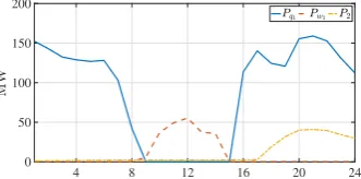
We assume that the cascade operates together with solar generation of250MW capacity. The solar generation and load data are depicted in Fig. 1.
B. Uncertainty modelling
We define the operation of the system for one day so that the net load is met. For these inputs, each of the hydroelectric power systems participates as shown in Fig. 2 which are the outcomes of (29). We notice that at the time where the net load is negative the pumped storage hydro plant is pumping the water as expected. In order to achieve maximum system efficiency, the first hydroelectric power station works to meet the load until the second hydro plant reaches its maximum volume and starts generating power at hour 18.
4 8 12 16 20 24
0 50 100 150 200
[image:6.595.104.229.606.694.2]4 8 12 16 20 24 -200
-100 0 100 200
[image:7.595.78.248.53.125.2]MW
Fig. 3: Sample paths of net load for a 24-hour period.
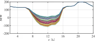
However, the actual output of the solar generation may be different than that forecasted. In Fig. 3, the output of various sample paths of the net load for forecast error of the solar output up to 30% are depicted. We run the optimal dispatch for the pumped storage hydro cascade as described in (29) for sample paths of the net load for forecast errors10-30%. Some representative results are depicted in Fig. 4. It may be seen in Fig. 4b that for higher forecast errors the value of the hourly head levels changes considerably for different sample paths. This is a result of different scheduling decisions based on the net load.
C. Influence of Uncertainty on Objective Function
In order to quantify how the uncertainty levels influence the value of the objective function, i.e., the head levels of the system, and the dispatch decisions we use the robust optimiza-tion formulaoptimiza-tion presented in (29). First, we need to build a reference case against which we will be comparing the robust optimization results. To this end, we run 500 experiments, i.e., Monte Carlo simulations, where the net load at periodt was drawn at random, according to the uniform distribution on the segment[(1−θ)Ps,(1+θ)Ps]wherePsis the solar output and θ is the “uncertainty level” characteristic for the experiment. We calculate the mean and standard deviation of the objective function, i.e., P24
t=1
P2
i=1hi(t)−
P24
t=1
P2
i=1M si(t), with
M = 108. This mean value of the objective function for the differentθ’s, when all the solar generation output were known to us in advance, is found by using (29) to determine the optimal solution and is referred to as the “ideal” case.
We solve the robust optimization problem given in (50) to determine the influence of uncertainty θ on the head levels of the system. To this end, we test the optimal solution of the equivalent tractable robust reformulation of (50) with the “ideal” case for uncertainty levels of 5−15%. The results are summarised in Table II. As expected, the less is the uncertainty, the closer is the objective function to the ideal ones.
VI. CONCLUSION
In this paper, we formulated the optimal dispatch of a pumped storage hydro system by maximising the energy per
cubic meter of water in the system by taking into account uncertainty. We incorporated the uncertainty sources into a robust variant of the dispatch problem. We used tools from robust optimization to reformulate the original intractable problem to an amenable form while preserving immunisation against uncertainty. In the case study, we validated the results of the robust optimization with Monte Carlo simulations and quantified the “cost” of uncertainty with a realistic system.
REFERENCES
[1] A. Beluco, P. K. de Souza, and A. Krenzinger, “A method to evaluate the effect of complementarity in time between hydro and solar energy on the performance of hybrid hydro pv generating plants,”Renewable
Energy, vol. 45, no. Supplement C, pp. 24 – 30, 2012.
[2] ——, “A dimensionless index evaluating the time complementarity between solar and hydraulic energies,” Renewable Energy, vol. 33, no. 10, pp. 2157 – 2165, 2008.
[3] H. I. Skjelbred, “Finding seasonal strategies for hydro reservoir schedul-ing under uncertainty,” inInternational Conference on Renewable
En-ergy Research and Applications (ICRERA), Oct. 2013, pp. 579–583.
[4] R. E. Oviedo-Sanabria and R. A. Gonzlez-Fernndez, “Short-term opera-tion planning of the itaipu hydroelectric plant considering uncertainties,”
inPower Systems Computation Conference (PSCC), Jun. 2016, pp. 1–6.
[5] A. Hamann, G. Hug, and S. Rosinski, “Real-time optimization of the mid-columbia hydropower system,”IEEE Transactions on Power
Systems, vol. 32, no. 1, pp. 157–165, Jan. 2017.
[6] A. C. TalitaDal Santo, “Hydroelectric unit commitment for power plants composed of distinct groups of generating units,”Electric Power Systems
Research, vol. 137, pp. 16–25, Aug. 2016.
[7] J. G.-G. Manuel Chazarra, Juan Ignacio Prez-Daz, “Optimal joint energy and secondary regulation reserve hourly scheduling of variable speed pumped storage hydropower plants,”IEEE Transactions on Power
Systems, vol. 33, pp. 103–115, Jan. 2018.
[8] D. Apostolopoulou and M. McCulloch, “Optimal short-term operation of a cascade hydro-solar hybrid system,”under review in IEEE
Trans-actions on Sustainable Energy.
[9] Y. Degeilh and G. Gross, “Stochastic simulation of utility-scale storage resources in power systems with integrated renewable resources,”IEEE
Transactions on Power Systems, vol. 30, no. 3, pp. 1424–1434, May
2015.
[10] D. Apostolopoulou and M. McCulloch, “Cascade hydroelectric power system model and its application to an optimal dispatch design,” in
IREP’ 2017 - 10th Bulk Power Systems Dynamics and Control Sympo-sium, Aug. 2017, pp. 1–6.
[11] K. Margellos and S. Oren, “Capacity controlled demand side man-agement: A stochastic pricing analysis,”IEEE Transactions on Power
Systems, vol. 31, no. 1, pp. 706–717, Jan. 2016.
[12] A. Ben-Tal, A. Goryashko, E. Guslitzer, and A. Nemirovski, “Adjustable robust solutions of uncertain linear programs,”Mathematical Program-ming, vol. 99, no. 2, pp. 351–376, Mar. 2004.
[13] M. Mbuthia, “Hydroelectric system modelling for cascaded reservoir-type power stations in the lower tana river (seven forks scheme) in kenya,” in3rd AFRICON Conference, Sep. 1992, pp. 413–416.
Uncertainty Tractable robustreformulation MeanIdeal caseStd Price of robustness 5% 4091.8
4,094.5
1.0293 0.07 %
10% 4085.6 2.0357 0.2 %
[image:7.595.107.479.609.699.2]15% 4077.2 2.9376 0.4 %
TABLE II: Head levels vs. uncertainty level.
4 8 12 16 20 24
134 134.5 135 135.5 136
(a)θ= 10%.
4 8 12 16 20 24
134 134.5 135 135.5 136
(b)θ= 30%.