Reactive control of a two-body point absorber using reinforcement learning

Reactive control of a two-body point absorber using reinforcement learning

E. Anderlini

, D.I.M. Forehand

, E. Bannon

, Q. Xiao

, M. Abusara

a_{Institute of Energy Systems, University of Edinburgh, Faraday Building, Colin Maclaurin Road, Edinburgh EH9 3DW, UK} b_{Wave Energy Scotland, 10 Inverness Campus, In verness IV2 5NA, UK}

c_{Department of Naval Architecture, Ocean and Marine Engineering, University of Strathclyde, 100 Montrose Street, Glasgow G4 0LZ, UK} d_{College of Engineering, Mathematics and Physical Sciences, University of Exeter, Penryn Campus, Penryn TR10 9FE, UK}

A R T I C L E I N F O

Keywords:

Reinforcement learning (RL) Q-learning

Reactive control Point absorber

Wave energy converter (WEC)

A B S T R A C T

In this article, reinforcement learning is used to obtain optimal reactive control of a two-body point absorber. In particular, the Q-learning algorithm is adopted for the maximization of the energy extraction in each sea state. The controller damping and stiffness coefficients are varied in steps, observing the associated reward, which corresponds to an increase in the absorbed power, or penalty, owing to large displacements. The generated power is averaged over a time horizon spanning several wave cycles due to the periodicity of ocean waves, discarding the transient effects at the start of each new episode. The model of a two-body point absorber is developed in order to validate the control strategy in both regular and irregular waves. In all analysed sea states, the controller learns the optimal damping and stiffness coefficients. Furthermore, the scheme is independent of internal models of the device response, which means that it can adapt to variations in the unit dynamics with time and does not suffer from modelling errors.

1. Introduction

Wave power is a renewable energy resource that can considerably contribute to the future energy generation thus reducing society’s dependence on fossil fuels. Although a potential of up to 2.1 TW of power has been estimated globally (Gunn and Stock-Williams, 2012), wave energy converter (WEC) devices are not economically viable yet, despite a large number of different designs having been suggested (Falc~ao, 2010). The design of an effective control strategy is fundamental in order to address this problem, since it can result in substantial gains in absor-bed energy without additional hardware costs.

Over the years, different control strategies have been proposed for the maximization of power extraction of WECs. A review of thefirst studies can be found inSalter et al. (2002), whileRingwood et al. (2014) pre-sents a review of recent techniques. From hydrodynamic considerations, complex-conjugate control would theoretically provide optimal energy absorption by achieving resonance between the WEC and the incident waves (Salter et al., 2002). Nevertheless, delivering optimal control may be infeasible in reality due to the associated excessive motions and loads in extreme waves. Hence, alternative suboptimal control schemes have been implemented, which include physical constraints on the motions,

forces and power rating of the device (Ringwood et al., 2014). Latching, declutching, model-predictive and simple-but-effective control are instances of real-time WEC control schemes. Firstly sug-gested byBudal and Falnes (1977), latching control achieves resonance conditions by adjusting the time period when the machine is locked in place through a dedicated mechanism (Babarit et al., 2004; Babarit and Clement, 2006). During the remaining part of the wave cycle, the device motions are linearly damped. Declutching control presents a similar concept, but in this case the power take-off (PTO) system is disconnected during part of the wave cycle through a by-pass valve (with hydraulic PTOs) as opposed to beingfixed in place (Babarit et al., 2009). Model predictive control applies at each time step the force that is expected to result in maximum energy absorption over a future time horizon (Brekken, 2011; Hals et al., 2011; Li and Belmont, 2014a; Richter et al., 2014). Simple-but-effective control obtains an estimate for the optimal controller force by modelling the current excitation force as a narrow-banded function (Fusco and Ringwood, 2013). These control strategies can include constrains on the motions and loading of WECs. While it is hard to scale latching control to farms of WECs, model pre-dictive control has been successfully implemented for multi-body devices and even small array problems (Richter et al., 2013; Oetinger and

* Corresponding author at: Institute of Energy Systems, University of Edinburgh, Faraday Building, Colin Maclaurin Road, Edinburgh EH9 3DW, UK. ** Corresponding authors.

E-mail addresses:[email protected](E. Anderlini),[email protected](D.I.M. Forehand),[email protected](E. Bannon),[email protected](Q. Xiao),M.Abusara@ exeter.ac.uk(M. Abusara).

Contents lists available atScienceDirect

Ocean Engineering

journal homepage:www.elsevier.com/locate/oceaneng

https://doi.org/10.1016/j.oceaneng.2017.08.017

Received 6 December 2016; Received in revised form 16 June 2017; Accepted 14 August 2017 Available online 24 August 2017

Maga~na, 2014; Li and Belmont, 2014b; Amann and Maga~na, 2015; Oetinger et al., 2015). However, model predictive control presents high computational requirements. Simple-but-effective control results in similar performance, but with a simpler implementation (Ringwood et al., 2014). Nevertheless, these methods are strongly affected by the accuracy of the prediction of the future wave excitation force, usually over a short time horizon, as well as of the model of the machine dy-namics (Ringwood et al., 2014).

Resistive and reactive control represent alternative types of schemes that rely on time-averaged sea states, so that stationary wave conditions are assumed (Salter et al., 2002). Numerical simulations are performed so as to obtain the PTO damping (resistive control) or combination of damping and stiffness (reactive control) that result in maximum energy absorption in each sea state (Nambiar, 2015). It is possible to include force saturation within the numerical model and displacement con-straints in the cost function. On the one hand, these techniques may present a lower efficiency as compared with on-line control schemes. On the other hand, resistive and reactive control are conceptually simple to understand, and they present much lower computational costs than real-time methods. Furthermore, they are easily scalable to multi-body or multiple-device problems, as for instance shown byNambiar (2015).

The aforementioned schemes suffer from a significant problem: the optimal control action is determined based on internal models of the body dynamics. Therefore, modelling errors can severely affect the per-formance of these algorithms, with significant drops in efficiency. In addition, these control strategies do not account for changes in the device dynamics over time, e.g. due to slow marine growth or sudden non-critical subsystem failures. For these reasons, the authors have pro-posed the application of reinforcement learning (RL) to resistive control in a previous work (Anderlini, 2016). With this machine learning algo-rithm, the controller learns the optimal PTO damping coefficient in every sea state directly from experience. Penalties for large displacements are included to prevent failures in extreme waves.

In this article, the developed control strategy based on RL is gener-alised to reactive control. Although WECs are expected to be deployed in arrays so as to exploit the advantage of economies of scale (Nambiar, 2015), we consider a single, axisymmetric device for simplicity. In particular, a more realistic WEC than that inAnderlini (2016)is analysed: a two-body point absorber, similar to the reference model 3 inNeary and Previsic (2014), Previsic et al. (2014) and Yu et al. (2015). Point ab-sorbers, which extract energy by resisting the motions of a smallfloating body subject to wave loading through a PTO system, represent a well-understood and simple offshore WEC technology (Falc~ao, 2010). The performance of the algorithm is assessed in both regular and irreg-ular waves.

2. Optimal reactive control of a point absorber

2.1. System description

In this work, the reference model 3 point absorber developed by Sandia National Laboratories is used as a case study. This decision is based on its realistic design, while it is still possible to approximate its motions with a simple model. Furthermore, it is well documented in the literature. The development of the WEC is described inNeary and Pre-visic (2014)in detail.Previsic et al. (2014)andYu et al. (2015)present experimental measurements that have been used to quantify its perfor-mance. The device is afloating, moored, axisymmetric point absorber that comprises of two bodies, whose relative motion due to wave exci-tation results in absorbed energy.

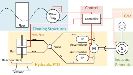
The selected point absorber features a hydraulic PTO system as shown inFig. 1, as envisioned byNeary and Previsic (2014). The mechanical energy associated with the relative motion between thefloat and the reaction plate is converted into electrical energy through a hydraulic stage. The advantages of a hydraulic PTO unit, whose design is inspired by Henderson (2006); Falc~ao (2007); Forehand et al. (2016), are its

robustness, capacity for energy storage and speed control. Furthermore, no expensive, fully-rated power converters are necessary because through the PTO system it is possible to control the output current (Forehand et al., 2016).

As shown inFig. 1, the point absorber comprises of two bodies: afloat and a reaction plate connected to a vertical spar. The wave excitation causes thefloat and reaction plate to move. However, the oscillations of the reaction plate present a much lower magnitude than thefloat because of the higher inertia, viscous drag and depth of the plate. Hence, the motion difference is used to drive a two-way, single-degree-of-freedom ram that pumps high-pressure oil into the circuit. A rectifying valve preventsflow reversal. Furthermore, theflow is smoothed out through a gas accumulator system. In the reference model 3 (Neary and Previsic, 2014), this comprises of four high-pressure (HP) cylinders and a low-pressure reservoir, designed to prevent cavitation (Forehand et al., 2016). Theflow drives a hydraulic motor, which is connected to an in-duction generator. The produced electrical power is fed into the national grid after the voltage is stepped up through a transformer.

As can be seen fromFig. 1, the input variables to the controller are the generated power,P, the displacement and velocity at the PTO,xPTOand

_

xPTO, respectively, and the wave elevation,ζ, from which the sea state is

derived. The controller then adjusts theflow in the hydraulic circuit by opening or closing the valves connected to the accumulators. This cor-responds to changing the damping and stiffness in the system.

2.2. Optimum reactive control

In reactive control, the controller force is calculated as the sum of a damping and a stiffness term [19]:

FPTOðtÞ ¼ BPTOx_PTOðtÞ CPTOxPTOðtÞ; (1)

wherexPTOis the displacement at the PTO. It is assumed that the PTO

damping and stiffness coefficients,BPTOandCPTO, respectively, can be

modified by changing the pressure within the hydraulic circuit. By varyingBPTOandCPTO directly, the developed algorithm can be easily

applied also to other PTO systems such as electromechanical or direct-drive.

In reality, the PTO force is saturated with a limitFMaxdue to the

generator rating, as shown inFig. 6inSection 4.1. The generated powerP can be calculated as:

PgenðtÞ ¼ FPTOðtÞx_PTOðtÞ; (2)

and the power fed into the grid is given by:

PðtÞ ¼ _η

Pgen ifPgen0; ðaÞ Pgen

η ifPgen<0: ðbÞ (3)

For simplicity, in(3)a single measure is employed for the overall efficiency of the PTO unit:η¼80% (Neary and Previsic, 2014). In(2),Pgen is the generated power. From(3)it is clear that with reactive control not

only is power extracted from the waves, but during part of the wave cycle it is also fed into the environment in order to increase the motions of the device through resonance and thus increase energy absorption (Salter et al., 2002). From this behaviour comes the name of the algorithm ”reactive control”.

The optimal PTO damping and stiffness coefficients that result in maximum energy extraction depend on the wave period in regular waves (Tedeschi et al., 2011) or the energy wave period,Te, in irregular waves.

If the force saturation is included, the optimumBPTOandCPTOvalues

become also functions of the significant wave height,Hs. Similarly, the

maximum displacement at the PTO, which is of interest to prevent fail-ures in extreme waves, is also a function of the sea state, given byHsand

Te.

The state-of-the-art optimum reactive control algorithm employs a tabular approach, where the optimal PTO damping and stiffness co-efficients are stored in a table for the main sea states that are encountered at the operational site, given by the combinations of a number of discrete values ofBPTOandCPTO. During the operation of the WEC, the controller

tries to achieve the prescribed PTO stiffness and damping coefficients in the current sea state through the hydraulic PTO system. The optimal coefficients are usually pre-calculated using an optimization algorithm, such as the Nelder-Mead simplex algorithm as inNambiar (2015), with a time-domain hydrodynamic model. For this reason, this technique can be affected by modelling errors and it cannot account for changes in the device response with time, e.g. due to ageing or marine biofouling.

3. Reinforcement learning control

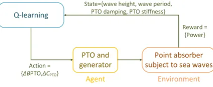
In reinforcement learning, the controller learns an optimal behaviour, orpolicy, from direct interaction with theenvironment. In this work, the on-line, off-policy Q-learning algorithm (Sutton and Barto, 1998) is selected as inAnderlini (2016). With this strategy, at each time stepnthe agent, which is in a specificstate sn, selects an actionan. As a result of the

interaction with the surrounding environment, the controller lands in a new state,snþ1, while observing areward,rnþ1, which depends on the

outcome of the chosen action. The action selection, modelled as a Markov decision process, depends on thevalue function, which is a measure of the expected future reward. By considering present as well as future rewards, RL is able to learn the optimal policy with time for the maximization of the total reward (Sutton and Barto, 1998).

Model-free RL techniques employ the action-value tableQ, which presents an entry for every combination of discrete states and actions. For instance,Qðsn;anÞrepresents the action-value for the current state and

action. The one-step update of the Q-learning algorithm is given by Sutton and Barto (1998):

Qnþ1ðsn;anÞ ¼Qnðsn;anÞ þαn

rnþ1þγmax_a02AQnðsnþ1;a0Þ Qnðsn;anÞ

; (4)

whereαnis defined as thelearning rate, which determines the proportion

of previous learning that is retained in the update of the action-value table, and γnis thediscount factor, which can be used to stress either

current or future rewards.

3.1. Application to the reactive control of wave energy converters

Fig. 2shows how Q-learning is used to learn the optimal combination of PTO damping and stiffness coefficients in each sea state without relying on any internal models of the device dynamics. At each step of the algorithm, the controller selects a step change in the coefficients (action), which is implemented by the PTO unit (agent). After interaction with the waves (the environment is represented by the point absorber subjected to ocean waves), the controller receives a reward, which is a function of the generated power, and moves to a new state, as given by the significant wave height, the energy wave period, and the PTO damping and stiffness coefficients.

The generated power must be averaged over multiple wave cycles so as to ensure transient effects from step changes inBPTOandCPTOdo not

affect the learning process. In particular, a longer time is required in irregular waves due to their random nature. Hence, the averaging is performed over a time horizon,H, during which the statesnand action an

are constant. As a result, the time steps of the Q-learning algorithm now have lengthH. As a new action is selected, there is an immediate change of state tosnþ1and a new averaging process.

3.1.1. State space

As aforementioned, the selected state variables are the significant wave height, the energy wave period, and the PTO damping and stiffness coefficients. Hence, the adopted RL state space is given by:

S¼ 8 > > < > > :s

jsi;j;k;l¼ ðHs;i;Te;j;BPTO;k;BPTO;lÞ;

i¼1:I; j¼1:J; k¼1:K; l¼1:L

9 > > = > >

;: (5)

The choice ofI, J, K, andL is based on a compromise between avoiding slow convergence associated with large values and ensuring sufficient learning accuracy, which may be affected by small values. In particular, due to the extra state variable as compared with resistive control (Anderlini, 2016) the learning time can become an issue with reactive control if large values are selected.IandJ are usually deter-mined by the wave resource at the deployment site. Typical ranges of the significant wave height and energy wave period areHs¼ ½0;9m and Te¼ ½5;14s, in steps of 1 m and 1 s, respectivelyHolthuijsen (2007). With a hydraulic PTO system, K and L are set by the number of accumulators.

3.1.2. Action space

For reactive control, the action is a combination of increase, decrease, or not change the PTO damping and stiffness coefficients. This gives 9 possible actions as opposed to only 3 in the case of resistive control (Anderlini, 2016). It has been preferred, however, to vary only one variable at a time in order to limit the action-state space thus decreasing the size of the Q-table. This has a direct consequence on the overall learning time. The action spaceAis now given by:

A¼ faj½ðΔBPTO;0Þ;ð0;ΔCPTOÞ;ð0;0Þ;ðþΔBPTO;0Þ;ð0;þΔCPTOÞg; (6)

whereΔBPTOandΔCPTOare predefined step changes in the PTO damping

and stiffness coefficients respectively.

The RL states corresponding to the minimum or maximum PTO damping and stiffness coefficients, i.e.BPTO;1,BPTO;K,CPTO;1andCPTO;L,

present a smaller action state to prevent the controller from exceeding the state space boundary. For instance, forCPTO;L, the actionΔCPTOis

invalid.

3.1.3. Reward

In this work, the same reward function, which represents the goal the controller needs to maximise, as inAnderlini (2016)is used. As shown in Fig. 2, the reward is dependent on the absorbed power. Nevertheless, the significant wave height can have stronger influence on the mean gener-ated power,Pavg, than variations inBPTOandCPTO. As a result,Pavg=H2sis

used instead because the absorbed power is proportional to the square of the significant wave height (Holthuijsen, 2007). Additionally, in order to help the learning process by filtering out the noise associated with random seas, the reward function is in fact based on the mean value of a numberMofPavgvalues (which are themselves time-averaged) for each

RL state. This is necessary because of the discretization of the state var-iables and the stochastic nature of irregular waves. Hence, theMmost recentPavg=H2s values are stored for each RL state in a matrix,R, which

presents at mostns⋅Mentries so as to prevent memory issues, wherensis

the total number of states, ns¼I⋅J⋅K⋅L. Thus, the mean value

corre-sponding to each state can be calculated and then expressed with the vectorm¼ hRðs;mÞim¼1:ðM_endÞof sizens, withhiindicating the averaging

process. In this vector, the states are arranged with a vectorised version of (5)so that the discrete values ofBPTOcorrespond to the innermost loop,

CPTOthe inner middle loop,Tethe outer middle loop andHsthe

outer-most loop.

In order to speed up the learning process, it is advantageous to present a cost function that is equal to one at the optimum and zero everywhere else. This is achieved by first normalizing the values of m by the maximum in each sea state, i.e. for the sameHsandTe. This means that

the maximum value is searched between the indices o¼floorððsn

1Þ=ðK⋅LÞÞ⋅K⋅Lþ1 andp¼floorððsn1Þ=ðK⋅LÞÞ⋅K⋅LþK⋅Lof the vectorm.

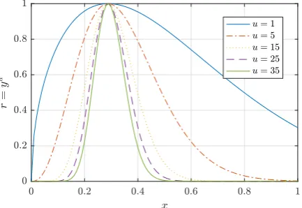
Then, the normalized values should be raised to a very high power,u¼25, so that the optimum will present a value of one and the other terms will tend to zero. This process is necessary because the location of the opti-mum is unknown, and results in the algorithm giving greater importance to the optimum over suboptimal PTO coefficients, even if they result in mean generated power with only a slightly smaller magnitude.Fig. 3 enables the user to fully understand this point, which is of primary importance in the derivation of a suitable reward function for the control of WECs. As an example inFig. 3, the reward function is assumed to be given by a Weibull distribution (Holthuijsen, 2007) with scale and shape parameters 0.6 and 1.5 respectively, whose values are normalized. From Fig. 3, it is clear that a greater value ofucorresponds to a more pro-nounced peakiness. However, a plateau is reached for large values.

Additionally, with reactive control, negative mean power values are possible, which may present a magnitude greater than the maximum power by which the corresponding value inmis normalized. In this case, it is best not to raise them to a power, so that a preliminary reward function is given by:

wðsnÞ ¼ 8 > > > < > > > :

_h

mðsnÞi

maxs¼o:phmðsÞi u

if mðsnÞ>0; ðaÞ

hmðsnÞi

maxs¼o:phmðsÞi if mðsnÞ 0: ðbÞ

(7)

For greater clarity, the calculation of the reward function is shown

graphically inFig. 4 for thefinal step of the RL algorithm using the simulation inFig. 10inSection 5.2. As is described inSection 5.2, this data is generated from running the algorithm in an 8-h-long wave trace in one sea state of irregular waves, which simulates the behaviour of the controller in a realistic scenario. Looking at the tableR, it is possible to make two observations. Firstly, despite the length of the wave trace being analysed (which corresponds to the duration of the controller operation), not all RL states (i.e. rows of the table) present fullyMentries, which means they have been encountered for less thanMtimes (withM¼25 in this simulation). Secondly, even for each state, the values ofPavg=H2scan present a wide range due to the variation in wave energy for the same discrete sea state. This is the main reason behind selecting a relatively large value ofM, which should result in outliers playing a minor role in the calculation of the vector of the mean values,m. InFig. 4, only one sea state is used, so that all entries ofmare normalized with respect to the maximum power. However, if more sea states were present, it would be sufficient to update the portion ofmcorresponding to the current sea state only as defined by indicesoandpin(7). Finally,Fig. 4shows that the use of a high value of the poweru, whereu¼25 is used in this case, results in a smaller reward being associated with suboptimal combina-tions of the PTO damping and stiffness coefficients, as expected from Fig. 3.

Furthermore, some combinations of PTO damping and stiffness co-efficients may result in large motions in extreme waves that may lead to failure. For this reason, a penalty,2, is returned whenever the magni-tude of the maximum displacement at the PTO exceeds a set value, xPTO;Max. Hence, the complete reward function is given by:

rnþ1¼

wðsnÞ ifjmaxðxPTOÞj xPTO;Max; ðaÞ

2 ifjmaxðxPTOÞj>xPTO;Max: ðbÞ (8)

3.1.4. Exploration strategy, learning rate and discount factor

Particularly at the start of the learning process, it is advantageous for the agent to try unseen actions in new states, which is a process known as exploration. As the learning progresses, the controller can shift towards the selection of actions that result in greater reward (exploitation), since there is greater confidence in their values. In this work, this has been achieved through anϵ-greedy exploration strategy, which results in the following action selection at each step of the Q-learning algorithm (Sutton and Barto, 1998):

an¼

argmaxa’2AQnðsn;a’Þ with probability 1ϵn; ðaÞ

random action with probabilityϵn: ðbÞ (9)

In order to ensure exploration at the start and then shift the focus to exploitation, the exploration rateϵn2 ½0;1is calculated as:

ϵn¼ _ϵ

0 if N0; ðaÞ

ϵ0

. ffiffiffiffi

N

p

if N>0; ðbÞ (10)

whereN¼Pi¼1:5Nnðsn;aiÞ Nminϵ, withna¼5 indicating the number of

actions.Nis the matrix containing the count of the number of visits to each state action pair,Nminϵis the minimum number of visits to each state

for an initial random exploration, andϵ0is the initial exploration rate.

The selection ofNminϵandϵ0should be based on a compromise. Higher

values of these variables ensure greater exploration (withϵ0¼1

indi-cating completely random initial actions) and thus increase the chances of the algorithm converging towards the optimum behaviour. At the same time, lower values, particularly forNminϵ, reduce the time during which random actions are taken, with the WEC exhibiting suboptimal performance. Hence, values of Nminϵ¼25 and ϵ0¼0:6 have been

selected as a good choice for the specific case study being analysed in this work. If a greater number of RL states is used, the value ofNminϵshould be

increased.

Similarly, the learning rateαn2 ½0;1 should also decrease as the

learning goes on. Nevertheless, a slower decay is sought in order to Fig. 3.Influence ofuon the peakiness of the reward function, based on the example of a

ensure the controller keeps on updating the Q-table throughout the exploration stage:

αn¼

α0 ifNnðsn;anÞ Nminα; ðaÞ

α0=Nnðsn;anÞ ifNnðsn;anÞ>Nminα; ðbÞ (11)

whereNminαindicates the number of visits to each state-action pair before

reducing the learning rate. As for the exploration rate, a higher learning rate aids the learning process, but a slower decay slows the convergence time of the state-action value function (Sutton and Barto, 1998). It is common practice to select the learning rate to be lower than the explo-ration rate. For this reason, α0¼0:4 is chosen. Additionally, Nminα<

Nminϵshould be selected because the decay of the exploration rate

de-pends on the number of visits to each state (for any actions), while that of the learning rate on the number of visits to each state-action pair. In the case of the presented reactive control, there are 5 actions for each state, so thatNminα¼Nminϵ=5 is chosen.

The learning and exploration rates should be reset on a predefined, regular basis so as to account for changes in the WEC dynamics over time, e.g. due to marine growth or non-critical subsystem failure. Furthermore, a discount factorγ¼0:95 is employed. This is used to discount only slightly the future rewards the Q-learning algorithm receives.

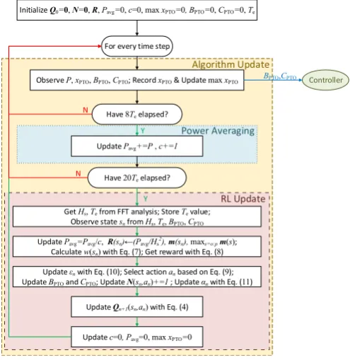
3.2. Algorithm

The proposed Q-learning algorithm for the reactive control of WECs can be seen inFig. 5. Thefirst step consists of the initialization of all variables.QandNare matrices of dimensionsnsna.Ris a vector of

vectors, whose dimensions are at mostnsM, withM¼10 in regular

waves andM¼25 in irregular waves. As inAnderlini (2016), the entries ofRare pre-calculated in a run in a similar wave trace, whilst taking random actions. It is expected thatRwill be pre-initialized using simu-lations also for the full-scale device: as the WEC begins to operate,Rwill be updated using actual sensor data. In addition, since some combina-tions of PTO damping and stiffness coefficients can result in very large motions, it is necessary to initialize the Q-table during a pre-training stage using simulations in order to prevent failure in extreme waves.

After the initialization stage, the algorithm is run indefinitely until maintenance is due. At every time step, the selected PTO damping and stiffness coefficients are implemented by the controller through the PTO system. Furthermore, the generated power and the displacement at the PTO are sampled in order to update respectively the mean absorbed power and the maximum displacement value in each time horizon. In particular, the power averaging is performed only after 8Tehave passed

in order to remove transient effects due to change inBPTOorCPTO. A

longer time is required than for resistive control in Anderlini (2016), since a change in PTO stiffness coefficient can cause large motions. Additionally, the time horizon lasts 20Tein both regular and irregular

waves. This results in a speed-up in convergence as compared with 30Tz

inAnderlini (2016), whilst still ensuring the algorithm is stable. FromFig. 5, the Q-learning update at the end of each episode can be seen. The values of the significant wave height and energy wave period are computed using spectral analysis and Fast Fourier Transforms (FFT) from the record of the wave elevation with a unidirectional wave spec-trum for simplicity(Holthuijsen, 2007).

4. Simulation system

4.1. Hydrodynamic model

The analysed WEC is described inSection 2.1and shown inFig. 1. Greater information on the device and its dimensions and properties can be found inNeary and Previsic (2014), Previsic et al. (2014) and Yu et al. (2015). Assuming linear wave theory and small body motions, the response of the device can be obtained from the superposition of the inertial, hydrostatic, viscous, radiation, diffraction and incident forces in addition to the control force (Falnes, 2005). The two-body problem can be thus modelled with a twelve-degree-of-freedom model. However, by Fig. 4.Calculating the rewardw(excluding penalties for large motions) at one step of the RL algorithm in irregular waves. This corresponds to the last step in 10 inSection 5.2.

considering only planar motion, i.e. surge, heave and pitch, and the axisymmetric geometry of bothfloat and reaction plate, which means heave is decoupled from surge and pitch (Falnes, 2005), it is possible to simplify the model to the coupled heave degrees of freedom of the two bodies. Therefore, using Cummins’formulation for the radiation force (Cummins, 1962), it is possible to express the equations of motion of the device in the time domain with the following matrix notation:

ðMþAð∞ÞÞ€xðtÞ þ∫t0KðtτÞx_ðτÞdτþCxðtÞ ¼fexðtÞ þfPTOðtÞ þfvðtÞ: (12)

M is the inertia matrix, which can be obtained using the data in Previsic et al. (2014), andCthe stiffness matrix. The calculation of the heave hydrostatic stiffness for thefloat is standard (Falnes, 2005), whose dimensions can be found inPrevisic et al. (2014), with the sea water densityρ¼1025 kg/m3

and the gravitational accelerationg¼9.81 m/s2 . The reaction plate and spar do not present any hydrostatic stiffness because they are fully submerged. Nevertheless, a stiffness term of 10 MN/m, which is likely to be provided by the mooring system, is specified in order to prevent an unstable behaviour with reactive control.

In(12),K is the radiation impulse response function matrix, and

Að∞Þthe added mass matrix at infinite wave frequency. These variables can be computed using the commercial program WAMIT, where the geometry is created following the dimensions inPrevisic et al. (2014). In particular, panels are included at the waterline within thefloat contour so as to remove the effects of irregular frequencies (WAMIT, 2013). Furthermore, the bottom is left with a hole where the top of the sparfits. Similarly, the top of the spar is left without panels. Care has been taken in ensuring there is a match in the position of the points lying on the inner border of the bottom of thefloat and on the outer border of the top of the spar to prevent errors in the solution. This arrangement results in incorrect volume and hydrostatic calculations, but in an accurate computation of the radiation and diffraction coefficients. In addition, the use of dipoles on the reaction plate has been found to result in in-stabilities in the radiation approximation, described hereafter. For this reason, it has been preferred to model the reaction plate as a thicker plate, with a thickness of 3 m (1/10th of the diameter (Previsic et al., 2014)). This approximation has been found to have only a minor effect on the radiation coefficients in heave.

In(12),fexis the excitation force vector, which is calculated from the

convolution of the excitation impulse response function, also obtained via WAMIT, and the wave elevation as described inFalnes (2005). Ac-cording to Newton’s 3rd_{law of action and reaction,f}

PTO¼ ½FPTO;FPTOT

is the controller force vector, withFPTObeing computed as in(1). For this

simple case, the displacement and velocity at the PTO can be obtained from the difference in the displacement and velocity of the two bodies: xPTOðtÞ ¼x3ðtÞ x9ðtÞ, where 3 and 9 indicate the heave degree of

freedom of thefloat and reaction plate respectively according to standard practice. The viscous drag force,fv, can be calculated with Morison’s

equation (Morison et al., 1950). While no drag force has been modelled on the water-piercing float, its contribution is expected to be non-negligible on the motions of the reaction plate. Since the magnitude of the velocity of the reaction plate is relatively small in all sea states analysed in this article, a constant drag coefficientCD¼5 is employed,

taken fromPrevisic et al. (2014).

Fig. 6shows the expression of(12)in a block diagram. In order to reduce the computational requirements of the hydrodynamic model, the radiation convolution integral is approximated by a state-space formu-lation as in (Anderlini, 2016). Frequency-domain system identification is employed so as to obtain state-space matricesAss,Bss,Css, andDss

ac-cording to the procedure described by Forehand et al. (2016), with

Dss¼0. The matrixDis used to calculate the viscous drag force. All its

entries are zero, except forD9;9¼0:5CDρπR2plate, whereRplate¼15 m is

the radius of the reaction plate (Previsic et al., 2014). In addition, the hydrodynamic model in Fig. 6 has been solved numerically using a

first-order accurate Euler scheme with a sampling time ofΔt¼0:1 s.

4.2. Simulation model

Numerical simulations have been run for the reference model 3 two-body point absorber, whose dimensions can be found inPrevisic et al. (2014). The maximum PTO force that can be exerted due to the generator rating has been assumed to beFMax¼1 MN, while the magnitude of the

maximum displacement at the PTO has been limited toxPTO;Max¼5 m.

The program employed for the simulations is summarized inFig. 7. While a buoy will record the wave elevation in practice as shown in Fig. 1, a wave model is used to generate the wave elevation time series in Fig. 7. On the one hand, the wave elevation is used to obtainHsandTe.

On the other hand, it is required for the calculation of the wave excitation force through the diffraction convolution integral (Falnes, 2005).

In order to generate the wave elevation in irregular waves, the amplitude wave spectrumSðωÞneeds to be specified for a number of circular wave frequencies (Holthuijsen, 2007),ω. The individual wave components are superimposed to calculate ζ, each having a wave amplitudeAðωÞ ¼pffiffiffiffiffiffiffiffiffiffiffiffiffiffiffiffiffiffiffi2SðωÞΔω, whereΔωis the circular frequency step (Falnes, 2005).Δωshould be selected smaller than the Nyquist frequency in order to prevent a repetition of the wave trace (Franklin et al., 2008). This is particularly problematic, since it is evident fromSection 5.2that very long wave traces are required for the RL algorithm to converge. For this reason, it has been preferred to generate the wave trace as the combination of 15-min long wave traces, where a different seed for the random number generator is used for each one. Furthermore, a 20-point

filter is used over the last andfirst 20 s of each trace in order to smoothen the connection. Therefore,Δω¼0:005 rad/s has been used, since it meets the Nyquist criterion (Franklin et al., 2008), which has been possible byfitting the diffraction coefficients generated by WAMIT with a high-order polynomial.

For simplicity, the PTO damping coefficient is assumed to range from Fig. 6.Block diagram used for the calculation of the motions of thefloat and reac-tion plate.

0 to 4.2 MNs/m in steps of 1.4 MNs/m, so thatK¼4. Similarly, the PTO stiffness coefficient is taken to range from3.6 MN/m to 0 MN/m in steps of 1.2 MN/m, so thatL¼4. These values have been selected as they fully enclose the optimal coefficients for the analysed sea states. As a result of the choice of PTO damping and stiffness coefficients, 16 RL states are used when a single sea state, as given by Hs and Te, is

considered. Nevertheless, for a more realistic implementation a finer resolution and a wider range are expected.

5. Simulation results

The learning capabilities of the algorithm are assessed in both regular and irregular waves. Since the same time horizon length has been selected in both cases, the same wave trace length of 8 h has been employed as opposed toAnderlini (2016), where a longer time series was required in irregular waves. The hydrodynamic model is initialized for 15 min to prevent numerical instabilities, although this trace is not re-ported in the plots. Additionally, the RL response is validated against optimal reactive control, whose coefficients are obtained from Nelder-Mead simplex optimizations (Nambiar, 2015) in 20-min-long wave traces.

5.1. Regular waves

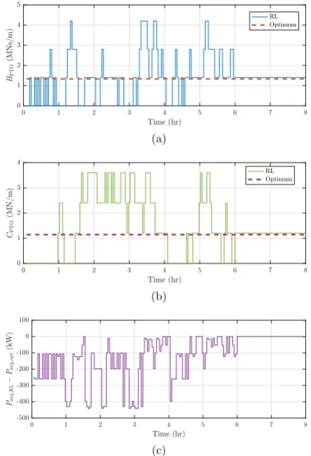
A single sea state, i.e.I¼J¼1, has been analysed in regular waves, with unit amplitude and a wave period of 8 sFig. 8a and b compare the curves of the PTO damping and stiffness coefficients respectively with time as selected by the Q-learning algorithm against the optimal values. The difference in the corresponding mean absorbed power and the optimal mean generated power of 260.5 kW can be seen inFig. 8c.

In addition, the reward function is plotted against the PTO damping and stiffness coefficients inFig. 9for the same sea state. In particular, two values have been used foru, the power of the normalized power in(7). Note that because the displacement limit is not reached,r¼win this case ((7) and (8)). The case ofu¼1 corresponds to purely the normalized mean generated power values, whileu¼25 is used in the actual cost function in this article.

5.2. Irregular waves

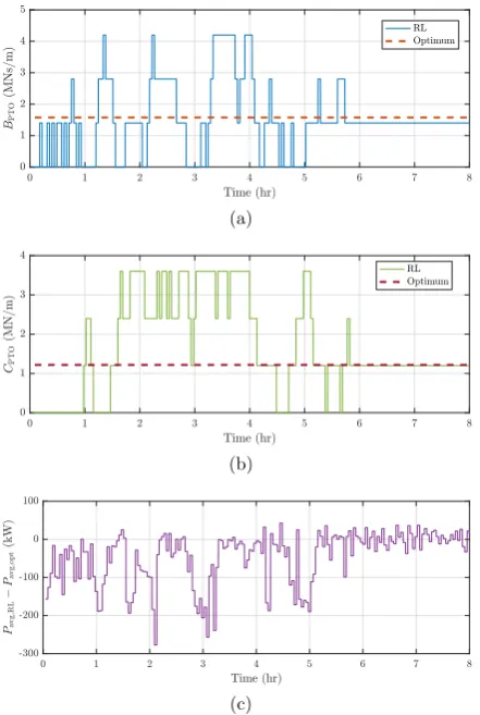
Similarly, a single sea state, with a significant wave height of 2 m and a peak wave period of 9.25 s is considered in irregular waves as a proof of concept. From the FFT analysis, the energy wave period for the generated wave trace is 8 s. As per the regular waves case,I¼J¼1 so that the RL problem reduces to 16 states.

InFig. 10a and b, it is possible to see the PTO damping and stiffness coefficients respectively adopted by the RL control scheme as compared with the optimal values in this sea state.Fig. 10c shows the difference in the corresponding mean absorbed power, with the mean generated power obtained by using the optimal coefficients being 90.582 kW.

6. Discussion

6.1. Regular waves

As is clear from Fig. 8, in regular waves the Q-learning algorithm learns the optimal PTO coefficients in approximately six hours from a random start (Q¼0). This is almost double the time required by the control scheme for resistive control inAnderlini (2016)mainly due to the longer time horizon employed: 20Teas opposed to 10Tz, with the energy

wave period being typically greater than the zero-crossing mean wave period. In fact, a shorter time horizon may be used considering the deterministic nature of regular waves. Additionally, the convergence time is strongly dependent on the number of discrete BPTO and CPTO

values employed, with only 16 states currently being used.

InFig. 8, it is also interesting to notice the random initial behaviour of

the controller due to the selected exploration strategy, which enables the agent to visit most states. As the learning progresses, the exploration rate tends to zero and the algorithm chooses the optimal, exploitative actions. In order to meet the requirements of the linear wave theory assumption of the hydrodynamic model, a short wave height has been chosen. As a result, the prescribed maximum PTO displacement is never exceeded. Hence, the penalty term in(8)is not applied. If it were, the controller would be expected to select a higher PTO damping coefficient, as inAnderlini (2016)for resistive control. Conversely, a PTO stiffness Fig. 8.Time variation of the PTO damping (a) and stiffness (b) coefficients chosen by the RL control as compared with the respective optimal values in regular waves of unit amplitude and a wave period of 8 s (c) shows the difference between the corresponding mean generated power and the optimal mean generated power.

coefficient with a smaller, if not zero, magnitude is forecast, as the controller tries to move away from resonance. On the other hand, the force reaches the saturation limit even in this mild sea state. However, a bang-bang behaviour similar to the one in Anderlini (2016) is not observed with reactive control.

InFig. 9, it is interesting to compare the developed cost function (u¼25) with the original normalized generated mean power surface (u¼1) for the same sea state. As can be seen, raising the non-dimensional power values to a high power results in a much peakier reward function, similar to what is observed inFig. 3for an example function. This is highly desirable, since it enables the controller to learn more quickly what the optimal action is, as there is a more significant gain associated with it as compared with suboptimal solutions. This results in a consid-erable speed-up in the convergence time as opposed to the case ofu¼1. Even higher values of the powerumay be required for afiner mesh of PTO damping and stiffness coefficients, since this can present aflatter region around the optimum. As aforementioned, this approach is necessary because the actual position of the optimum is unknown, with the best reward function in terms of convergence time being the one that presenting a value ofþ1 at the optimum and 0 everywhere else.

It is important to notice that raising negative normalized mean generated power values to a high value ofuis strongly undesirable. This would have the effect of decreasing the magnitude of the reward as for positive power values, but in this case it would actually mean increasing the reward associated with suboptimal points. It would be even worse to use an even value for u, since it would turn negative mean generated power values into positive ones, thus teaching the controller a completely wrong policy. Hence, positive values ofufor negative normalized mean generated power values must be avoided at all costs.

6.2. Irregular waves

From Fig. 10, it is evident that the developed statistical reward function is effective in ensuring convergence in irregular waves as well, despite their stochastic nature. Furthermore, since the same horizon time length is employed as per the regular waves run, the learning time is no greater as opposed to the study byAnderlini (2016). Nevertheless, the challenge that irregular waves pose to the convergence of the correct action selection can be understood by comparingFig. 8c andFig. 10c, where the much more oscillatory nature of the mean absorbed power in irregular waves is clear.

A typical sea state has a duration that ranges between 30 min and 6 h (Holthuijsen, 2007). Hence, even though the learning time is smaller than inAnderlini (2016)despite the larger number of states, convergence is still unlikely to be achieved before there is a variation in the significant wave height and energy wave period. However, as shown inAnderlini (2016)for irregular waves with multiple sea states, the Q-learning al-gorithm applied to the control of WECs is able to pick up the learning process from where it left off the last time it encountered a particular sea state. This represents the main advantage of reinforcement learning over traditional optimization algorithms, which would be unable to identify whether a change in the cost function is due to a change in the PTO damping or stiffness coefficients or due to noise in the wave energy.

In a realistic application, afiner grid ofBPTOandCPTOvalues would be

desired in order to deal with a large range of sea states. Nevertheless, this may increase the learning time excessively. The Q-table is expected to be pre-initialized through numerical simulations in order to prevent selecting PTO settings that result in excessive motions in energetic sea states, which could be a real problem with reactive control. In addition, the exploration and learning rates should be reset every season so as to check if there have been variations in the device response over time, e.g. due to slow marine growth or abrupt non-critical subsystems failure. Since the operational life of WEC technologies is envisioned to be 20–25 years, a relatively poor performance during the initial stages of operation should be more than offset by increases in the absorbed wave power throughout a devices operating life through the removal of modelling errors.

Finally, it is important to understand that RL is proposed as a method to remove the dependence of existing WEC control strategies from hy-drodynamic models. In RL, the controller is independent of the plant. In this work, a hydrodynamic model based on potentialflow theory with some non-linear, viscous effects is used to simulate the plant. Neverthe-less, as shown for instance inAnderlini (in preparation) for resistive control, RL control is able to converge towards the optimal policy even in the presence of strong non-linear effects associated with the PTO system. Hence, due to its model-free nature, RL is expected to perform well even when applied to non-linear numerical models, such as CFD, or even in experimental or prototype testing. However, the overall controller per-formance is only as good as the control scheme itself, with reactive control representing a significant improvement over resistive control treated in the previous study (Anderlini, 2016).

7. Conclusions

The authors have presented an on-line, model free strategy for the reactive control of WECs using RL, building on a previous study on resistive control. The algorithm has been validated through a numerical model of a two-body point absorber which assumes linear wave theory. In both regular and irregular waves the controller is shown to learn the optimal PTO damping and stiffness coefficients that result in maximum energy absorption. In order to achieve convergence in irregular waves, a statistical reward function has been developed, which averages over multiple mean absorbed power values in each sea state. As the control scheme is independent of internal models of the device response, it is simple to implement on a real, full-scale WEC. Additionally, it can adapt to variations in the machine conditions over time, e.g. due to ageing or Fig. 10.Time variation of the PTO damping (a) and stiffness (b) coefficients chosen by the

marine biofouling. Although the Q-table has been randomly initialized, in a real application it is expected to be pre-calculated through simula-tions in order to prevent the adoption of acsimula-tions that may cause failures in extreme waves. The action-values will then be slowly substituted by the actual measured data during operation with corresponding necessary adjustments. Finally, this method, which has already been generalised to the application to multi-body devices in this work since a previous study (Anderlini, 2016), can be further extended to the treatment of arrays of devices.

Acknowledgements

The authors would like to thank the Energy Technologies Institute (ETI) and the Research Councils Energy Programme (RCEP) for funding this research as part of the IDCORE programme (EP/J500847/), as well as the Engineering and Physical Sciences Research Council (EPSRC) (grant EP/J500847/1). In addition, Mr. Anderlini would like to thank Wave Energy Scotland (WES) for sponsoring his Eng.D. research project. WES is taking an innovative approach to supporting the development of wave energy technology by managing the most extensive technology programme of its kind in the sector, concentrating on key areas which have been identified as having the most potential impact on the long-term levellised cost of energy and improved commercial viability.

References

Amann, K.U., Maga~na, M.E., Member, S., Sawodny, O., 2015. Model predictive control of a nonlinear 2-body point absorber wave energy converter with estimated state feedback. IEEE Trans. Sustain. Energy 6 (2), 336–345.

Anderlini, E., Forehand, D.I.M., Stansell, P., Xiao, Q., Abusara, M., 2016. Control of a point absorber using reinforcement learning. Trans. Sustain. Energy 7 (4), 1681–1690.

Anderlini, E., Forehand, D.I.M., Bannon, E., Abusara, M., 2017. Control of a realistic wave energy converter model using least-squares policy iteration. IEEE Trans. Sustain. Energy.https://doi.org/10.1109/TSTE.2017.2696060in preparation.http:// ieeexplore.ieee.org/document/7911321/.

Babarit, A., Clement, A.H., 2006. Optimal latching control of a wave energy device in regular and irregular waves. Appl. Ocean Res. 28 (2), 77–91.https://doi.org/ 10.1016/j.apor.2006.05.002.

Babarit, A., Duclos, G., Clement, A.H., 2004. Comparison of latching control strategies for a heaving wave energy device in random sea. Appl. Ocean Res. 26 (5), 227–238.

https://doi.org/10.1016/j.apor.2005.05.003.

Babarit, A., Guglielmi, M., Clement, A.H., 2009. Declutching control of a wave energy converter. Ocean Eng. 36 (12–13), 1015–1024.https://doi.org/10.1016/ j.oceaneng.2009.05.006.

Brekken, T.K.A., 2011. On Model Predictive Control for a point absorber Wave Energy Converter. In: Proceedings of the IEEE Trondheim PowerTech, 1–8.hhttp://dx.doi. org/doi:10.1109/PTC.2011.6019367i.

Budal, K., Falnes, J., 1977. Optimum operation of wave power converter. Mar. Sci. Commun. 3 (2), 133–150.

Cummins, W.E., 1962. The impulse response function and ship motions. Schiffstechnik 47 (9), 101–109.

Falc~ao, A.F.D.O., 2007. Modelling and control of oscillating-body wave energy converters with hydraulic power take-off and gas accumulator. Ocean Eng. 34 (14–15), 2021–2032.https://doi.org/10.1016/j.oceaneng.2007.02.006.

Falc~ao, A.F.D.O., 2010. Wave energy utilization: a review of the technologies. Renew. Sustain. Energy Rev. 14 (3), 899–918.https://doi.org/10.1016/j.rser.2009.11.003.

Falnes, J., 2005. Ocean Waves and Oscillating Systems, Paperback Edition. Cambridge University Press.

Forehand, D., Kiprakis, A.E., Nambiar, A., Wallace, R., 2016. A bi-directional wave-to-wire model of an array of wave energy converters. IEEE Trans. Sustain. Energy 7 (1), 118–128.https://doi.org/10.1109/TSTE.2015.2476960.

Franklin, G.F., Powell, J.D., Emami-Naeini, A., 2008. Feedback Control of Dynamic Systems, 6th edition. Pearson.

Fusco, F., Ringwood, J.V., 2013. A simple and effective real-time controller for wave energy converters. IEEE Trans. Sustain. Energy 4 (1), 21–30.https://doi.org/ 10.1109/TSTE.2012.2196717.

Gunn, K., Stock-Williams, C., 2012. Quantifying the potential global market for wave power. In: Proceedings of the 4th International Conference on Ocean Engineering (ICOE 2012) 1–7.

Hals, J., Falnes, J., Moan, T., 2011. Constrained optimal control of a heaving Buoy wave-energy converter. J. Offshore Mech. Arct. Eng. 133 (1), 011401.https://doi.org/ 10.1115/1.4001431.

Henderson, R., 2006. Design, simulation, and testing of a novel hydraulic power take-off system for the Pelamis wave energy converter. Renew. Energy 31 (2), 271–283.

https://doi.org/10.1016/j.renene.2005.08.021.

Holthuijsen, L.H., 2007. Waves in Oceanic and Coastal Waters. Cambridge University Press.

Li, G., Belmont, M.R., 2014. Model predictive control of sea wave energy converters - Part I. A convex approach for the case of a single device. Renew. Energy 69, 453–463.

https://doi.org/10.1016/j.renene.2014.03.070.

Li, G., Belmont, M.R., 2014. Model predictive control of sea wave energy converters - Part II. The case of an array of devices. Renew. Energy 68, 540–549.https://doi.org/ 10.1016/j.renene.2014.02.028.

Morison, J., Johnson, J., Schaaf, S., 1950. The force exerted by surface waves on piles. J. Pet. Technol. 2 (5), 149–154.https://doi.org/10.2118/950149-G.

Nambiar, A.J., Forehand, D.I.M., Kramer, M.M., Hansen, R.H., Ingram, D.M., 2015. Effects of hydrodynamic interactions and control within a point absorber array on electrical output. Int. J. Mar. Energy 9, 20–40.https://doi.org/10.1016/j.ijome.2014.11.002. Neary, V.S., Previsic, M., Jepsen, R.a., Lawson, M.J., Yu, Y.-H., Copping, A.E., Fontaine, A.a., Hallett, K.C., 2014. Methodology for Design and Economic Analysis of Marine Energy Conversion (MEC) Technologies. Tech. Rep. March, Sandia National Laboratories.hhttp://dx.doi.org/10.0/SAND2014-9040i.

Oetinger, D., Maga~na, M.E., Member, S., Sawodny, O., 2014. Decentralized model predictive control for wave energy converter arrays. IEEE Trans. Sustain. Energy 5 (4), 1099–1107.

Oetinger, D., Maga~na, M.E., Sawodny, O., 2015. Centralised model predictive controller design for wave energy converter arrays. IET Renew. Power Gener. 9 (2), 142–153.

https://doi.org/10.1049/iet-rpg.2013.0300.

Previsic, M., Shoele, K., Epler, J., 2014. Validation of theoretical performance results using wave tank testing of heaving point absorber wave energy conversion device working against a subsea reaction plate. 2nd Marine Energy Technology Symposium, 1–8.

Richter, M., Magana, M.E., Sawodny, O., Brekken, T.K.a., 2013. Nonlinear model predictive control of a point absorber wave energy converter. IEEE Trans. Sustain. Energy 4 (1), 118–126.https://doi.org/10.1109/TSTE.2012.2202929.

Richter, M., Sawodny, O., Magana, M.E., Brekken, T.K.a., 2014. Power optimisation of a~ point absorber wave energy converter by means of linear model predictive control. IET Renew. Power Gener. 8 (2), 203–215.

https://doi.org/10.1049/iet-rpg.2012.0214.

Ringwood, J.V., Bacelli, G., Fusco, F., 2014. Energy-maximizing control of wave-energy converters. The development of control system technology to optimize their operation. IEEE Control Syst. Mag. 34 (5), 30–55.

Salter, S.H., Taylor, J.R.M., Caldwell, N.J., 2002. Power conversion mechanisms for wave energy. Proc. Inst. Mech. Eng. Part M 216 (1), 1–27.https://doi.org/10.1243/ 147509002320382112.

Sutton, R.S., Barto, A.G., 1998. Reinforcement Learning. Hardcover Edition, MIT Press. Tedeschi, E., Carraro, M., Molinas, M., Mattavelli, P., 2011. Effect of control strategies

and power take-off efficiency on the power capture from sea waves. IEEE Trans. Energy Convers. 26 (4), 1088–1098.https://doi.org/10.1109/TEC.2011.2164798. WAMIT, 2013. User Manual: Version 7.0,arXiv:1011.1669v3,hhttp://dx.doi.org/10.

1017/CBO9781107415324.004i.