https://doi.org/10.1007/s00190-019-01265-7 O R I G I N A L A R T I C L E
Demonstrating developments in high-fidelity analytical radiation force
modelling methods for spacecraft with a new model for GPS IIR/IIR-M
S. Bhattarai1 ·M. Ziebart1·S. Allgeier2·S. Grey3·T. Springer4·D. Harrison1·Z. Li1
Received: 21 August 2017 / Accepted: 2 June 2019 © The Author(s) 2019
Abstract
This paper presents recently developed strategies for high-fidelity, analytical radiation force modelling for spacecraft. The performance of these modelling strategies is assessed using a new model for the Global Positioning System Block IIR and IIR-M spacecraft. The statistics of various orbit model parameters in a full orbit estimation process that uses tracking data from 100 stations are examined. Over the full year of 2016, considering all Block IIR and IIR-M satellites on orbit, introducing University College London’s grid-based model into the orbit determination process reduces mean 3-d orbit overlap values by 9% and the noise about the mean orbit overlap value by 4%, when comparing against orbits estimated using a simpler box-wing model of the spacecraft. Comparing with orbits produced using the extended Empirical CODE Orbit Model, we see decreases of 4% and 3% in the mean and the noise about the mean of the 3-d orbit overlap statistics, respectively. In orbit predictions over 14-day intervals, over the first day, we see smaller root-mean-square errors in the along-track and cross-track directions, but slightly larger errors in the radial direction. Over the 14th day, we see smaller errors in the radial and cross-track directions, but slightly larger errors in the along-track direction.
Keywords Solar radiation pressure·Analytical force models·GPS·Orbit determination·Orbit prediction
1 Introduction
At Global Navigation Satellite System (GNSS) altitudes, the major force that affects satellite trajectories is Earth gravity, but the effects of solar and lunar gravity are also considerable. Next in this hierarchy of forces, as shown in Fig. 3.1 of Mon-tenbruck and Gill (2000), there is solar radiation pressure (SRP), which is caused by the interaction of solar photons with spacecraft surfaces. If this is not accounted for in the force models used for orbit prediction, the calculated position of the spacecraft can be in error at the 100-m level after 12 h (Fliegel and Gallini1996). For this reason, SRP modelling is an important topic in GNSS orbit determination and precise
B
S. Bhattarai [email protected]1 Department of Civil, Environmental and Geomatic Engineering, University College London, London, UK 2 ATA Aerospace, Albuquerque, USA
3 Department of Mechanical and Aerospace Engineering, University of Strathclyde, Glasgow, UK
4 PosiTim UG, Seeheim-Jugenheim, Germany
orbit determination (POD) in general (Montenbruck and Gill
2000; Vallado and McClain2001; Tapley et al.2004). Since the 1980s, various methods for dealing with the problem have been presented in the literature (Colombo
1986; Beutler et al.1994; Fliegel and Gallini1996; Springer et al.1999; Bar-Sever and Kuang2003; Arnold et al.2015). Many of these are empirical methods, requiring no a priori knowledge of the spacecraft properties or its operating envi-ronment. In global network analyses that incorporate tracking measurements from a large network of one hundred stations or more, such methods can produce spacecraft orbits with cm-level accuracy (So´snica et al.2015).
approach, first introduced by Marshall and Luthcke (1994) for application to POD of the TOPEX/Poseidon mission, has been particularly influential. The general concept is to model the spacecraft structure using eight flat plates (six for a cuboid representing the spacecraft bus and two for solar panels), with assumed values for the optical and thermal properties of the surfaces, which are then combined with a priori mod-elling of the spacecraft attitude and the incident radiation fluxes. This approach was applied to the Block II/IIA and Block IIR satellites of the Global Positioning System (GPS) by Rodriguez-Solano et al. (2012). In comparing the perfor-mance of their semi-analytical adjustable box-wing model with the Centre for Orbit Determination (CODE) Empiri-cal Orbit Model (ECOM; Beutler et al.1994), the authors determined that the orbit solutions produced by the two meth-ods were comparable, but that the accelerations produced by the ECOM model were less physically meaningful. More recent efforts that adopt a broadly similar modelling approach include Montenbruck et al. (2015) for Galileo satellites and Montenbruck et al. (2017a) for the QZS-1 satellite of Quasi-Zenith Satellite System (QZSS).
The box-wing models are relatively easy to implement. However, they are not able to fully capture the radiation flux-spacecraft surface interaction in satellites with complex surface geometry where the effects of mutual self-shadowing and reflected radiation can be significant. An alternative class of analytical radiation force modelling methods, in which ray-tracing techniques are combined with detailed spacecraft surface models to account for SRP, Earth radiation pres-sure (ERP) and thermal re-radiation (TRR), was developed in the early 1990s (Klinkrad et al.1991), and these meth-ods are able to capture these detailed effects. The models were tested in POD of the European remote sensing satellites ERS-2 and ENVISAT (Doornbos et al. 2002). To distin-guish them from the box-wing methods, we refer to these as high-fidelity analytical radiation force modelling methods. In GNSS, high-fidelity SRP modelling for GLONASS satel-lites was first explored by Ziebart and Dare (2001). This work was motivated by broader efforts to improve GLONASS orbit quality as part of the IGEX-98 campaign (Willis et al.
1999). Work in this area continued over the years at Uni-versity College London (UCL), where the approach was enhanced with methods to account for TRR (Adhya2005), ERP (Sibthorpe2006; Ziebart et al. 2007; Li et al. 2017) and antenna thrust (AT; Ziebart et al.2007), and validated on a number of additional cases including the GPS Block IIA and Block IIR satellites, the Jason-1 spacecraft of the Ocean Surface Topography Mission and ENVISAT (Ziebart et al.2005; Sibthorpe2006). Recent work in this area demon-strated improved accuracy in shadow modelling when using geometric primitives, as opposed to triangular tessellations, to represent curved surfaces when constructing the spacecraft model (Grey and Ziebart2014). The modelling approach, as
presented in Ziebart et al. (2005), was adopted into the opera-tional standards for precise orbit determination of the Jason-1 altimetry satellite (Cerri et al.2010; Zelensky et al.2010). Recently, other research groups have explored a broadly sim-ilar approach for modelling SRP on Beidou satellites (Tan et al. 2016; Wang et al. 2018), on the Gravity Field and Steady-State Ocean Circulation Explorer (GOCE) satellite (Gini2014) and on QZS-1 (Darugna et al.2018).
In this paper, using a new model for the GPS Block IIR and IIR-M satellites, we present developments to the UCL model computation strategies that are designed to extend the valid-ity of the models to all possible orientations of the radiation source(s) with respect to the spacecraft. As such, these next-generation general-purpose models account for the effect of radiation forcing from any number of radiation sources, from any direction, providing a high-fidelity radiation flux–space-craft interaction model that can be used to deal with both SRP and ERP. A key advantage of this approach is that the final model makes no prior assumptions about the attitude characteristics of the spacecraft and can therefore deal with any deviations from nominal attitude.
2 UCL modelling strategy
Our radiation force modelling strategy comprises three pro-cesses:
(i) Computation of the bus model, where the space vehi-cle bus contribution to the accelerations due to SRP and ERP is dealt with. In this process, the accelerations due to thermal emissions from the multi-layered insulation (MLI) covering the bus are also computed, according to Sect. 4.3.3 of Adhya (2005). The core technique uses a ray-tracing algorithm, where the rays simulate the incident radiation flux for a given geometry of the spacecraft with respect to the radiation source. The out-put of this process is a set of three grids representing the accelerations in theX,Y andZ-axes of the space-craft body-fixed system (BFS), where the grid nodes are spaced at 1° intervals in latitude and longitude in the BFS.
(ii) Separate computation of the solar panel model, where the solar panel contributions to the accelerations due to SRP and ERP are dealt with.
(iii) AT modelling, which accounts for the recoil force on the spacecraft due to emission of photons from signal transmitters.
built from a combination of geometric primitives (polygons, circles, cylinders, spheres, cones and truncated cones), avoid-ing any need for tessellation, especially on curved surfaces (Ziebart et al.2003). This produces models with good geo-metric fidelity without requiring an excessively large number of components, e.g. the UCL model for the GPS IIR/IIR-M bus, as shown in Fig.6, is made up of 182 components. The solar panels (not shown in Fig.6) are modelled as two rect-angular plates.
For solar flux, the models are computed using a nomi-nal value for the mean solar irradiance at one astronomical unit (AU) of 1368 Wm−2(Hastings and Garrett1996). The solar irradiance is known to vary over the solar cycle (with a period of between 9 and 14 years) by 1.4 Wm−2. This
repre-sents circa 0.1% variation in the parameter. Little is gained by correcting the nominal value. It is more important to scale the model depending on the probe-Sun distance at the calcu-lation epoch. Taking 1368 Wm−2as a reference value, the eccentricity of the Earth’s orbit about the Sun modulates the solar irradiance near the Earth to 1415.7 Wm−2at perihelion (+3.4%) and 1322.6 Wm−2at aphelion (−3.3%). This gives a variation (between perihelion and aphelion) of circa 100 Wm−2(the precise value being 91.3 Wm−2), approximately 6.7% of the mean value.
For the Earth radiation flux model, we use data from the Clouds and Earth Radiant Energy System (CERES) (Wielicki et al. 1996) project, which provides the irradiance at the top-of-atmosphere (TOA), an altitude of ~ 30 km above the Earth’s surface, in a grid format spaced at 1-degree inter-vals in latitude and longitude in an Earth-centred Earth-fixed (ECEF) system. Computationally, it can be expensive and slow to determine the total Earth radiation flux incident on a spacecraft, from the part of the Earth’s surface that is visible to that spacecraft, based on a search of the full CERES grid. To overcome this, we have developed a configurable Earth radiation model that re-organises the CERES data into a grid of triangles wrapped around the TOA surface. The number of triangles used to represent the TOA surface is configured during run-time, based on the number of triangles required to achieve a specified precision level. This approach is outlined in Li et al. (2017). At GNSS altitudes, radiation flux from the Earth is about 15 Wm−2.
In the ray-tracing algorithm, a pixel array (simulating the radiation source) is projected onto the computer simulation of the spacecraft with the force at each ray-surface intersection computed according to:
Fn −
E A c cosθ
(1 +μν)cosθ+2
3ν(1−μ)
ˆ
n, (1)
Fs
E A
c cosθ[(1−μν)sinθ]sˆ
, (2)
Fmli
2σTmli4
Anˆ and (3)
Tmli4 αEcosθ+effσT 4 sc
σ(mli+eff) ,
(4)
where
• Fnis the normal force acting in the direction of the surface
normal,nˆ,
• Fs is the shear force acting in theˆs direction, which is
along the projection of the total force onto the surface plane,
• Fmliis the force due to the thermal re-radiation from the
MLI on the bus surface, which also acts along the normal direction,
• E is the mean irradiance of the radiation source at one astronomical unit,
• Ais the area of the surface (determined in this case by the pixel array spacing),
• cis the speed of light in vacuum,
• νis the reflectivity of the material,
• μis the specularity of the material,
• θis the angle of incidence of the radiation with respect to the surface,
• Tmliis the temperature of the MLI, • σis the Stefan–Boltzmann constant,
• αis the absorptivity of the MLI material,
• mliis the emissivity of the MLI material,
• eff is the effective emissivity between the MLI and the
spacecraft and
• Tscis the internal temperature of the spacecraft bus.
Note, Eqs.1and2are derived in Ziebart (2001,2004) and Eqs.3and4are developed in detail in Adhya (2005). The acceleration due to AT,x¨at(r,t), is calculated according to:
¨
xat(r,t) W
mcˆr, (5)
whereWis the signal power in Watts,mis the spacecraft mass in kg andˆris the unit vector from the geocentre towards the satellite centre of mass (Ziebart et al.2007).
2.1 Bus model computation scheme
To produce the complete bus model, the pixel array is rotated around the spacecraft in a systematic way, through a discrete set of points, and the ray-tracing computations are performed from each point. Each computation takes the following form:
f(ϕ, λ) ⎡ ⎣aaxy
az ⎤
⎦, (6)
where the inputsϕ atan2
z, x2+y2andλatan2
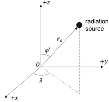
(y,x)represent latitude and longitude, respectively, of the radiation source in the spacecraft BFS (as defined in Fig.1); the outputsax,ayandazare acceleration along theX,Yand Z-axes, respectively, in the spacecraft BFS.
In the computation scheme used in early analyses (Ziebart and Dare2001), the pixel array was rotated around the space-craftY-axis at 12° intervals in the Earth-probe-Sun (EPS) angle, as shown in Fig. 2. The ray-tracing algorithm was executed at 30 points only, and a Fourier series was fitted to the results to represent the final continuous model. The underlying assumption was of spacecraft attitude behaviour fully consistent with the nominal attitude model, in which the Sun is confined to the XZ plane, and theZ-axis points to the geocentre (see Fig.2). In subsequent studies, e.g. Ziebart et al. (2005), this modelling assumption was maintained but the number of data points computed was increased to 360 by reducing the increment in the EPS angle to 1°.
GNSS satellites on orbit may depart from a nominal atti-tude state due to limitations of their attiatti-tude control systems.
Fig. 1 Defining latitude and longitude in the spacecraft BFS. Here,ϕ∈ (−90◦,+90◦)and is defined byϕ ∈ (0◦,180◦), according toϕ 90◦−ϕwhereϕis the angle between theZ-axis (in the +Z-direction) andrs, wherersis the position of the radiation source in the spacecraft BFS;λ∈ (−180◦,+180◦)is the angle between theX-axis (in the + X-direction) and the projection ofrson theX–Yplane and it is positive in the anticlockwise direction and negative in the clockwise direction
Fig. 2 In nominal attitude mode, in the spacecraft BFS, the Sun is con-fined to the BFSX–Z plane and the spacecraft Z-axis points to the geocentre
Non-GNSS satellites can have attitude laws that are far less constrained than the typical GNSS attitude laws. Thus, as the application of the core technique was considered for non-GNSS missions, the computation scheme was modi-fied. First, the EPS-sweep pixel array orientation scheme was proposed. In this scheme, the pixel array centre points are uni-formly distributed around the spacecraft in the central EPS plane (i.e. the spacecraftX–Zplane in this case). Then, each point is rotated by±1° about the spacecraftY-axis, resulting in a new set of points, all inclined at±1° with respect to the spacecraftX–Z plane. This process is repeated at 1° steps to populate a full set of pixel-array centre points in 10°-arcs around the spacecraft as shown in Fig.3. For GNSS satel-lites, the EPS-sweep method produces pixel arrays that are distributed around the primary parts of the spacecraft BFS within which the Sun moves, but coverage remains incom-plete in other directions.
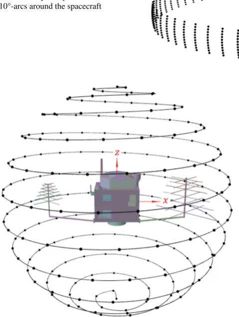
Therefore, an additional computation scheme based on the spiral points algorithm (Saff and Kuijlaars 1997) was introduced, see Fig.4. With this method, it is possible to effi-ciently position the radiation source uniformly on a sphere that encloses the spacecraft. As it provides complete coverage in all directions, it can be used to produce a general-purpose model that makes no prior assumptions about the orientation of the spacecraft with respect to the radiation source(s). Cur-rently, the spiral points computation scheme is our preferred model computation method, but there are additional data pro-cessing steps required before the outputs of a computation scheme based on this method can be used in a POD process.
2.2 Producing the grid files
[image:4.595.333.507.55.199.2] [image:4.595.77.256.470.638.2]Fig. 3 A visualisation to demonstrate the EPS-sweep pixel array centre point orientation scheme. Here, there are 792 points representing a discrete sample of points on 10°-arcs around the spacecraft
Fig. 4 A visualisation to demonstrate the spiral points computation scheme with 200 spiral points. Each point represents a pixel array centre point for a single instance of a radiation pressure acceleration compu-tation and for the specific geometry of the radiation source with respect to the spacecraft
0◦) and ending at the south pole (ϕ −90◦, λ0◦). This is not a standard method for organising the data. Thus, to provide a final model that is easily integrated into the POD processes of model users, we produce a set of acceleration grids, with grid nodes uniformly spaced at 1° intervals in latitude and longitude in the satellite frame.
To compute the grid values, we use a modified ver-sion of Shepard’s method (Shepard1968)—specifically, an implementation of the modified quadratic Shepard’s method (Franke and Nielson1980) with a type of full sector search as described in Renka (1988)—to determine the optimal set of gridding parameters. The interpolated values are com-puted in a two-step process. First, a quadratic surface is fitted around each data point. The quadratic (Q) neighbours param-eter dparam-etermines the radius of a circle large enough to include the nearestQneighbours. Then, the interpolant at a chosen
location is computed using an inverse distance weighted aver-age of the computed quadratic surface fits around each data point. The weighting (W) neighbour’s parameter specifies the number of nearest data points to include for this. There are no clear rules for choosing either theQor theW param-eter for the modified Shepard’s method, in that the optimal choice is data set specific. In this work, for the GPS IIR bus model, we developed a quality assurance process for deter-mining this parameter pair using a two-dimensional search throughQ–W space. This is how the process works:
(i) The radiation pressure model is computed using the spiral points scheme and the EPS-sweep scheme. (ii) The 10,000 spiral points data set is expanded using a
padding process, see below.
(iii) Using modified Shepard’s method, 1600 grids are pro-duced from the output of the spiral points computation, for each acceleration component, with all combinations ofQ,W pairs considered, where bothQandW range from 11 to 50.
(iv) For each grid file, the interpolated values at each of the 3960 EPS-sweep points are calculated, and the inter-polated value is compared with the results from the EPS-sweep computation. This is used to compute the RMS error value,Erms, for that grid file according to:
Erms
1
3960
3960
k1
(aEPS,i−agrid,i)2, (7)
whereaEPS,iare accelerations at pointiaccording to the
EPS-sweep computation andagrid,i is an interpolated
acceleration at pointiderived from the grid file. (v) Finally, the grid files that minimise the Ermsquantity
for each component (X,Y andZ) are chosen as the optimal grid files for that spacecraft.
2.3 Padding the spiral points data set
[image:5.595.52.292.113.432.2]spec-ified set of the nearest neighbour points. As such, in using this method to create the radiation force model grids, we encounter a problem. The algorithm is not able to identify the correct nearest neighbour points in the regions close to the data set boundaries (i.e. ϕ 90◦or −90◦, λ 180◦or−180◦) when the output from a spiral points com-putation, labelled using latitude and longitude pairs in a 2-d Cartesian system, is provided as the input. To overcome this, we developed a method that creates an artificially extended spiral points data set that is bounded in the region ϕ ∈
(−270◦,+270◦)andλ ∈ (−540◦,+540◦). The transforma-tion rules that map the raw spiral points data, bounded in the regionϕ ∈ (−90◦,+90◦)andλ∈ (−180◦,+180◦), to data points in the extended regions are given in Eqs.8to15, where f(ϕ, λ)is used to populate the extended region using the raw data. A portion of this extended data set around the north pole (ϕ 90◦) is shown in Fig.5, where the red data points are the spiral points. The yellow points, the top-padding above the north pole, are reflections of the raw data points about the
ϕ90◦line, which are then shifted by±180◦in longitude beyond the north pole. Using this, expanded data set gives us a solution to the nearest neighbour problem. Another largely unavoidable issue is caused by the requirement to project the spiral points onto a 2-d Cartesian space, which distorts the apparent distance between points. With the Mercator projec-tion, this effect increases with distance fromϕ 0◦. The impact of this is clearly seen in Fig.5where the density of data points becomes sparser approachingϕ90◦.
Top-padding (T):ϕ >90◦,λ∈(−180◦,180◦)
f(ϕ, λ)
f(180◦−ϕ, λ−180◦) forλ≥0
f(180◦−ϕ, λ+ 180◦) forλ <0 (8)
Bottom-padding (B):ϕ <−90◦,λ∈(−180◦,180◦)
f(ϕ, λ)
f(−180◦−ϕ, λ−180◦) forλ≥0
f(−180◦−ϕ, λ+ 180◦) forλ <0 (9)
Left-padding (L):ϕ ∈(−90◦,90◦), λ <−180◦
f(ϕ, λ) fϕ, λ+ 360◦ (10)
Right-padding (R):ϕ ∈(−90◦,90◦), λ >180◦
f(ϕ, λ) f(ϕ, λ−360) (11)
Top-Left Padding (TL):ϕ >90◦, λ <−180◦
f(ϕ, λ) f180◦−ϕ, λ+ 180◦ for λ∈−360◦,−180◦
(12)
Top-Right Padding (TR):ϕ >90◦, λ >180◦
f(ϕ, λ) f180◦−ϕ, λ−180◦ for λ∈180◦,360◦ (13)
Bottom-Left Padding (BL):ϕ <−90◦, λ <−180◦
f(ϕ, λ) f−180◦−ϕ, λ−180◦ for λ∈−360◦,−180◦
(14)
Bottom-Right Padding (BR):ϕ−90◦, λ+ 180◦
f(ϕ, λ) f−180◦−ϕ, λ−180◦ for λ∈180◦,360◦
(15)
2.4 Modelling limitations
There are a number of factors limiting the accuracy of the current approach, which include:
(a) Mis-modelling of reflected radiation coming off the bus onto the panels and shadowing from the bus onto the panels (and vice versa). Both of these are due to the separate treatment of the solar panels and the spacecraft bus during model computation. Here, there is a trade-off in modelling accuracy between being able to deal with non-standard solar panel orientations and being able to capture the effects of reflections and self-shadowing of the bus onto the panels. An analysis of this trade-off is not presented here but will be considered carefully in future development work.
(b) No modelling of the time-evolution of the surface mate-rial properties.
(c) Incomplete modelling of TRR effects. In the ray-tracing algorithm, we only consider spacecraft bus surfaces that are covered in multi-layer insulation (MLI). This strat-egy can perform reasonably well on those satellites where the surfaces are mostly covered in MLI, as is the case with the GPS Block IIR and IIR-M bus sur-faces. However, it is limited in cases where a significant
proportion of the spacecraft surface is not covered in MLI (e.g. the SAR antenna on Sentinel-1; radiators on Galileo spacecraft, etc.). Also, we are not considering the force due to the temperature gradient across the Sun-facing and anti-Sun-Sun-facing sides of the solar panels in this study, but this effect has been considered in previ-ous studies (Adhya2005) and we are working towards developing a simplified approach to account for this. (d) No modelling of thermal recoil forces due to emissions
from radiators and other thermal control system com-ponents that actively emit heat. The impact of this will be different between the Block IIR and the Block IIR-M satellites. The thermal control system of the Block IIR-M satellites was updated with additional integral heat pipes due to high heat concentrations in the honeycomb structure of the L-band panel due, in part, to increased signal power needs (Hartman et al.2000).
3 Model implementation
The UCL radiation force model implementation requires sev-eral inputs. Most of these are spacecraft-specific information that includes position, nominal mass, actual mass if available, the grid files for the bus model, solar panel properties (area, surface material properties), attitude information (in the form of attitude control laws or on-board attitude measurements) to enable accurate determination of the spacecraft BFS and solar panel orientation in the BFS.
As explained in Sect.2, the model for the spacecraft bus is pre-computed, with the results of the computation stored in grids that are uniformly spaced at 1° intervals in latitude and longitude of the Sun position in the spacecraft BFS. To call these models in an orbit determination algorithm, these grids must be read in and stored in a suitable data structure. As a part of this process, it is a good idea to denormalise the grid values according to:
x¨grid mn maE ¨
xgrid, (16)
where
• mnis the nominal mass of the spacecraft, i.e. the value
used to compute the grid in kg,
• mais the actual mass of the spacecraft in kg,
• x¨gridare the grid file accelerations in the spacecraft BFS x,yandz-axes in ms−2,
• x¨gr i d are denormalised grid file accelerations in ms−2, • Eis the mean solar irradiance at 1 AU.
This is because our radiation force modelling software was originally developed for solar radiation pressure modelling
only. As such, the accelerations given in the grid files are produced using a solar radiation flux model that assumes a constant solar irradiance of 1368 Wm−2at 1 AU. However, by applying this denormalisation step, it becomes relatively straightforward to use the UCL grids as a general-purpose radiation flux-spacecraft interaction model.
With all required inputs provided, and made accessible, it is possible to compute the accelerations due to the separate model components. The bus model is computed according to:
¨
xbus(r,t)κEs(r,t)x¨grid(ϕs, λs)+Ee(r,t)x¨grid(ϕe, λe),
(17)
where κ is the shadow crossing function (equals 1 in full phase of the Sun and 0 in umbra);Es(r,t)andEe(r,t)are
solar radiation flux and Earth radiation flux, respectively, at the spacecraft’s locationrat timet;ϕsandλsare latitude and
longitude, respectively, of the Sun’s position in the spacecraft BFS;ϕeandλeare latitude and longitude, respectively, of the
Earth’s position in the spacecraft BFS. For latitude and lon-gitude values between grid nodes, the accelerations should be calculated using bilinear interpolation. The solar panel’s contribution to accelerations due to radiation forcing is:
¨
xpanel(r,t)κx¨panel,srp(r,t)+x¨panel,erp(r,t). (18)
Finally, the combined acceleration due to radiation forces, ¨
xrad, is calculated according to:
¨
xrad(r,t)x¨bus(r,t)+x¨panel(r,t)+x¨at(r,t), (19)
wherex¨at(r,t)is the acceleration due to antenna thrust.
4 The GPS IIR/IIR-M model description
and data sources
Fig. 6 A visualisation of the UCL computer model of a GPS Block IIR/IIR-M spacecraft bus that includes the NAP UHF antenna
Table 1 GPS IIR/IIR-M solar panel and yoke arm surface material prop-erties that are used in the UCL radiation pressure models
Properties Value
Solar array
Apanelm2 13.59
νfront 0.28
νrear 0.11
μfront 0.85
μrear 0.50
Yoke arms
Ayokem2 0.32
νyoke 0.85
μyoke 0.85
Values given to 2 decimal places (dp)
(Adhya2005). Thus, in our model, the same material prop-erties are used, i.e.ν 0.06 andμ0. The authors were unable to determine the full form on the NAP acronym or the purpose of this antenna.
The computation of the force models for the bus is per-formed using Version 5.05 of UCL’s Analytical SRP and TRR Modelling Software at a nominal spacecraft mass of 1100 kg and a pixel-array resolution of 1 mm2. The bus model grid files for the IIR/IIR-M spacecraft, with and without the NAP antenna, are provided alongside this article as an electronic supplement.
Most of the values used for our solar panel model, given in Table1, are taken from Adhya (2005). The combined surface area of the solar panel yoke arms is taken from Fliegel and Gallini (1996) because the drawings in Adhya (2005) provide only their length. For the rear side of the panels, we use surface properties given in Rodríguez-Solano (2009).
[image:8.595.50.289.280.440.2]In Table2, we present the statistics for the selected UCL grids for the GPS IIR/IIR-M satellites, both with and without
Table 2 Statistics relating to the selection of the grid files that represent the radiation pressure model for the GPS IIR/IIR-M spacecraft bus
Grid Q W RMS error Max error Bias
GPS IIR/IIR-M, with NAP antenna
X 37 13 0.0304 0.247 0.000370
Y 50 50 0.0351 0.320 −0.000610
Z 32 11 0.1580 2.710 0.002210
GPS IIR/IIR-M, no NAP antenna
X 34 13 0.0309 0.240 0.000353
Y 50 50 0.0352 0.323 −0.000858
Z 32 11 0.1590 2.726 0.002202
Units: nms−2
the NAP antenna. The grids chosen are the ones correspond-ing to theQ,Wparameter pairs that minimise the RMS error when the interpolated grid file values are compared against the results of an EPS-sweep computation. The RMS errors of theZ grids are approximately five times higher than the X grids. This is due to the W-band antennae and for those satellites that have them, the NAP antenna. In the EPS-sweep computation, these protruding elements result in significantly larger cross-section boundaries as the pixel array pans across theZ surfaces. By contrast, these elements have almost no effect on cross-section boundaries as the pixel array pans across the X surfaces. Thus, there are larger errors in the ray-tracing algorithm when computingZaccelerations. This is due to the edge-matching effect, which depends upon the cross-section perimeter and is explained in Chapter 10 of Ziebart (2001). This does not affect theY grids as the pixel arrays do not pan across theY surfaces in the same way.
[image:8.595.306.545.281.404.2]surface area of the solar array and yoke arms is 13.91 m2. In the ESOC BW model, for the surface properties of the bus,
ν0.06 andμ 0. The solar panel properties of the BW model and the UCL model are identical.
For the antenna thrust model, we use the IGS model values for signal power (http://acc.igs.org/orbits/thrust-power.txt), which are 85 W for GPS Block IIR and 108 W and 198 W for GPS Block IIR-M satellites.
5 Model validation
We investigate the performance of the new modelling strat-egy using two software systems: the UCL Orbit Dynamics Library (UCL-ODL) and ESOC’s Navigation Package for Earth Observation Satellites (NAPEOS) software (Springer
2009). The UCL-ODL comprises a set of programs devel-oped by researchers at UCL over the years, for the explicit purpose of studying the impact of force modelling strategies that are developed by the UCL Space Geodesy and Nav-igation Laboratory. NAPEOS is a GNSS data processing package developed by ESOC and used in its contributions to IGS activities to produce satellite orbits, precise clocks, station coordinates, Earth rotation parameters and so on.
5.1 Analysis of the impact of separate model
components using the UCL-ODL
Using the UCL-ODL, we performed a series of sensitivity analyses to investigate the impact of the individual model components and verify the implementation method. In these tests, as the reference trajectory, we used precise IGS final orbits, considering all available IIR and IIR-M satellites over the full month of March 2016. For each satellite, we perform multiple orbit predictions, with separate prediction runs cor-responding to separate IGS final orbit files. As such, in this part of the analysis, we consider 13 GPS IIR satellites and 7 GPS IIR-M satellites. For those satellites with a complete set of IGS final orbits during the analysis period, we perform 31 prediction runs from 1 to 31 March 2016. In the orbit propa-gator, the general force modelling strategy uses Earth Gravity Model 2008 up to degree and order 20 (Pavlis et al.2012,
2013) and the JPL Development Ephemerides 405 (DE405) for third-body gravitational forcing due to the Sun, Moon, Jupiter and Venus (Standish1998). The solid Earth tide effect due to the Sun and the Moon is accounted for according to Marsh et al. (1987). General relativistic effects are modelled according to Sect. 3.7.3 of Montenbruck and Gill (2000). The numerical integration is based on an 8th order Runge–Kutta integrator.
In terms of radiation force modelling strategy, the follow-ing scenarios were systematically assessed:
• Base model: SRP-only model using the ESOC BW model (Garcia-Serrano et al.2016).
• Test 1: SRP-only, where the bus model comprises grids produced by the UCL ray-tracing software, but only Eqs.1
and2are used.
• Test 2: Same as Test 1, but here the bus model comprises grids that account for both SRP and the effects of MLI TRR (Eqs.3and4).
• Test 3: Same as Test 2, but with ERP turned on.
• Test 4: Same as Test 3, but with AT turned on.
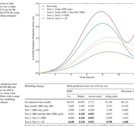
In Fig.7, we show the impact of different modelling strate-gies on orbit prediction error over a single 12-h arc for the GPS satellite SVN 46. As smaller and smaller effects are considered in the modelling strategy, the orbit prediction results improve, giving a general indication that the mod-els are performing as we expect. In Table3, we provide orbit prediction errors statistics for all Block IIR/IIR-M satellites on orbit during the analysis period. The best results, in the sense that the RMS and the maximum 3-d orbit prediction error over a 12-h arc are minimised, at 0.648 m and 1.440 m, respectively, are produced by the method that considers the combined effects of SRP, bus MLI TRR, ERP and AT. For that modelling approach, the full set of statistics for all satel-lites that were considered in the analysis, are given in Table4. An interesting observation from these results is that the mod-elling of the bus MLI TRR, an effect that is not considered by most IGS analysis centres, has a significant impact on reducing orbit prediction error over the arc.
5.2 Analysis of the impact of the new bus model
on POD using NAPEOS
Fig. 7 Comparison of orbit prediction error over a single instance of a 12-h arc for the GPS IIR satellite SVN 46, using different modelling strategies
Table 3 Orbit prediction error statistics for all GPS IIR and IIR-M satellites on orbit in March 2016 (i.e. mean value across all satellites) with a range of radiation force modelling strategies considered
Modelling strategy Orbit prediction error over 12-h arc (m)
RMS Maximum 3-d
3-d Radial Across-track Along-track
No radiation force model 44.272 14.951 2.711 41.150 96.131 Base model: SRP-only, BW 5.655 1.907 0.355 5.253 12.418 Test 1: SRP-only, grids 2.990 1.020 0.188 2.769 6.685 Test 2: SRP and Bus MLI TRR, grids 0.674 0.220 0.052 0.627 1.443 Test 3: Test 2 + ERP 0.650 0.220 0.052 0.599 1.447 Test 4: Test 3 + AT 0.648 0.220 0.052 0.598 1.440
Bold values indicate the lowest value error statistics among the various modelling strategies being compared Units: m
(Petit and Luzum2010). The numerical integration uses the Adams–Bashforth/Adams–Moulton 8th order prediction— correction multistep method, as described in Springer (2009). With the core data processing strategy fixed, we run the POD process using four different orbit modelling strategies, batch processed at 24-h intervals, from 00:00:00 to 23:59:30 in GPS time, thus completely independent from day to day. For the orbits, we generate estimates for the midnight epoch, such that there is an overlap between consecutive solutions at a single point. A full year (2016) is considered, so there are 366 independent solutions and 365 overlap points. In addition to the orbit model parameters, station coordinates and Earth rotation parameters are also estimated. The orbit models considered include:
1. ECOM: No a priori radiation force model, only the reduced ECOM (Springer et al. 1999) and three con-strained along-track parameters (constant, cosine and sine with argument of latitude as argument). Here, the
along-track parameters are included as soak-up parame-ters to absorb the effects of orbit mis-modelling, which tends to manifest strongly in the along-track direction, as the results of Sect.5.1demonstrate.
2. ECOM + BW: Same estimation strategy as ECOM-only, but here we also include an a priori radiation force model using the ESOC BW model of the GPS IIR and IIR-M spacecraft (Garcia-Serrano et al.2016).
3. ECOM + UCL: Here, the only difference with the ECOM + BW strategy is that the box is replaced by the grid-based model.
[image:10.595.97.538.48.461.2]Table 4 Orbit prediction error statistics for all GPS IIR and IIR-M satel-lites on orbit in March 2016
PRN SVN Orbit prediction error over 12-h arc
RMS Maximum
3-d Radial Across-track
Along-track
3-d
IIR
2 61 0.871 0.237 0.062 0.835 1.851 4* 49 1.325 0.290 0.028 1.293 2.380 11 46 0.632 0.219 0.064 0.588 1.586 13 43 0.137 0.038 0.072 0.107 0.245 14 41 0.923 0.244 0.070 0.888 1.921 16* 56 0.563 0.219 0.027 0.516 1.426 18* 54 0.731 0.220 0.019 0.687 1.367 19 59 1.143 0.333 0.044 1.093 2.560 20* 51 0.545 0.207 0.037 0.497 1.365 21 45 0.273 0.126 0.034 0.237 0.685 22* 47 0.432 0.175 0.030 0.392 1.125 23 60 0.574 0.275 0.076 0.496 1.706 28* 44 0.688 0.158 0.038 0.669 1.288 IIR-M
5* 50 0.760 0.256 0.029 0.712 1.740 7 48 0.689 0.171 0.088 0.662 1.133 12* 58 0.471 0.234 0.059 0.404 1.024 15 55 0.759 0.390 0.048 0.649 2.189 17 53 0.239 0.160 0.068 0.164 0.786 29 57 0.844 0.186 0.080 0.819 1.404 31 52 0.371 0.260 0.079 0.252 1.023 Mean 0.648 0.220 0.052 0.598 1.440 SD 0.295 0.076 0.021 0.302 0.575 The pseudorandom noise (PRN) code assigned to those satellites during the analysis period is indicated. Here, the radiation force modelling strategy that accounts for the effects of SRP, bus MLI TRR, ERP and AT is applied. Satellites in eclipse season during the analysis period are indicated with an asterisk (*) in the PRN column. Units: m
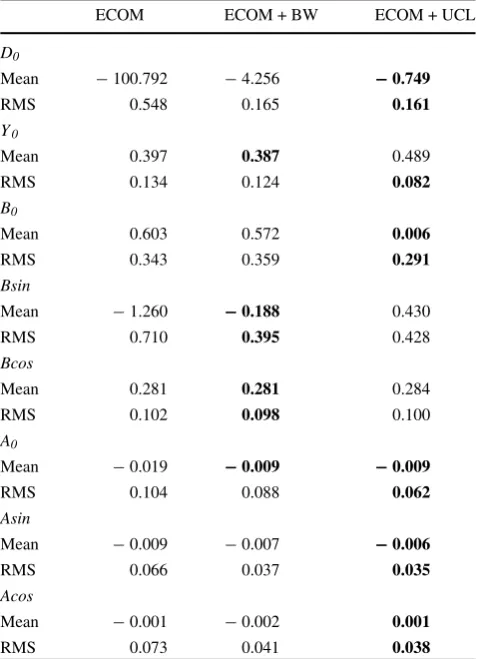
In Table 5, we present statistics of the estimated ECOM parameters from methods 1–3. We do not present the statis-tics for ECOM-2 because comparison between models with different parameterizations cannot be made directly. In gen-eral, as the daily solutions are fully independent of each other, smaller absolute values for both the mean and the RMS indicate an improvement in the force modelling. Using the ECOM + UCL model, we see a reduction in the absolute value of both the mean and the RMS values of theD0,B0
and all along-track parameters (except the mean of the A0
parameter that is the same for both), when comparing with results using the ECOM + BW model. We see a reduction in the RMS of theY0parameter, but the mean increases. The
[image:11.595.306.545.92.422.2]mean and RMS of the Bsin and Bcos parameters increase,
Table 5 Statistics of daily, independent estimates of the ECOM param-eters from three orbit modelling strategies for GPS Block IIR and IIR-M satellites over the full year of 2016
ECOM ECOM + BW ECOM + UCL
D0
Mean −100.792 −4.256 −0.749
RMS 0.548 0.165 0.161
Y0
Mean 0.397 0.387 0.489
RMS 0.134 0.124 0.082
B0
Mean 0.603 0.572 0.006
RMS 0.343 0.359 0.291
Bsin
Mean −1.260 −0.188 0.430
RMS 0.710 0.395 0.428
Bcos
Mean 0.281 0.281 0.284
RMS 0.102 0.098 0.100
A0
Mean −0.019 −0.009 −0.009
RMS 0.104 0.088 0.062
Asin
Mean −0.009 −0.007 −0.006
RMS 0.066 0.037 0.035
Acos
Mean −0.001 −0.002 0.001
RMS 0.073 0.041 0.038
Bold values indicate the lowest value error statistics among the various modelling strategies being compared
Units: nms−2
which indicate the presence of systematic effects that the ECOM + UCL combination is not effectively dealing with.
In Table6, we show the statistics of the orbit overlap dif-ferences. A smaller value for both the mean and the RMS indicates an improvement in the force modelling. The RMS values in all components are smallest with ECOM + UCL approach. However, the mean values for both the radial and along-track components are smallest with the ECOM-2 approach and the mean value for the cross-track component is smallest with the ECOM approach. In the 3-d orbit overlap values, we see a drop of 9% and 4% in the mean and RMS values, respectively, when we compare the ECOM + UCL results against ECOM + BW.
Table 6 Orbit overlap difference statistics from a comparison of GPS Block IIR and IIR-M orbits produced for daily, independent estimates using four different orbit modelling strategies over 2016
ECOM ECOM + BW ECOM + UCL ECOM-2
Radial
Mean 2.68 −0.30 −1.16 0.09
RMS 24.19 21.10 18.82 20.71
Along-track
Mean −4.74 −2.79 −2.82 2.03
RMS 32.00 27.94 26.37 26.79
Cross-track
Mean −0.02 −0.19 −0.40 0.13
RMS 23.28 19.47 18.17 18.41
Bold values indicate the lowest value error statistics among the various modelling strategies being compared
Units: mm
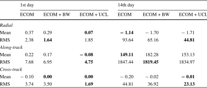
14 days, after the end of the 3-day fit interval. These predicted orbits were compared against the estimated orbits, on the first day and the last day of the prediction interval. In these tests, ECOM + UCL is the reference model and the orbits estimated using ECOM + UCL are used as the basis of the 3-day orbit fit and as the ground truth. These tests are done over 2016. Thus, the first 1-day prediction interval considered is day 4 of 2016 and the first 14th-day prediction interval is day 17. The results from these tests are presented in Table7.
Comparing RMS orbit prediction errors using ECOM + UCL against ECOM + BW, after 1-day, we see the errors increase by 0.21 cm in the radial direction but fall by 2.20 cm and 1.81 cm in the along-track and cross-track directions, respectively. For the 14th day predictions, we see a reduction in the RMS orbit prediction errors of 20.35 cm and 13.79 cm in the radial and cross-track directions, but an increase of 15.52 cm in the along-track direction. Overall, these results suggest ECOM + UCL is outperforming ECOM + BW, in the day 1 and day 14 orbit prediction tests, but there are lim-itations to this analysis that should be addressed in future
work for improved confidence in our findings. For example, because we use it as our reference model, it is possible that ECOM + UCL is favoured in these tests. Also, systematic errors, such as those that depend on the elevation of the Sun above the orbital plane, do not show up in the yearly statistics. A more complete picture of the comparative performance of the models should be investigated through time series anal-ysis.
6 Conclusions and discussion
Recent developments to our radiation force modelling strat-egy were analysed using a new model for the GPS Block IIR and Block IIR-M satellites. Advances to our approach include: an enhanced bus model computation scheme (based on the spiral points algorithm) that uses ray-tracing to deter-mine the radiation flux-spacecraft interaction from 10,000 points distributed uniformly on a sphere surrounding the spacecraft; an improved method (from a numerical stability perspective) for producing grids spaced at 1◦×1◦intervals in latitude and longitude in the spacecraft frame using a padding process to extend the spiral points data in all directions to reduce the impact of edge effects; a quality assurance pro-cess that uses results from an EPS-sweep computation with 3960 points for selecting an optimal set of grids. The models produced, and the proposed implementation method, were refined using a series of verification tests within the UCL-ODL. The impact of introducing UCL’s grid-based model into a full POD process was investigated by analysing the statistics of estimated orbit model parameters, orbit overlaps and orbit prediction errors. Combined, the results provide a good indication that introducing high-fidelity analytical force modelling into the POD process can improve the quality of the estimated orbits and further refinements of the approach to address current limitations are worth pursuing.
One of the difficulties with the high-fidelity approach lies in acquiring the spacecraft data (geometry, surface material
Table 7 Error statistics for day 1 and day 14 orbit predictions for GPS Block IIR and IIR-M orbits produced using three different orbit modelling strategies for 2016
1st day 14th day
ECOM ECOM + BW ECOM + UCL ECOM ECOM + BW ECOM + UCL
Radial
Mean 0.37 0.29 0.07 −1.14 −1.70 −1.71
RMS 2.38 1.64 1.85 93.64 65.16 44.81
Along-track
Mean 0.22 0.17 −0.08 149.11 182.28 153.13
RMS 7.68 6.95 4.75 1847.44 1819.45 1834.97
Cross-track
Mean −0.10 0.00 0.00 −0.20 −0.02 −0.01
RMS 3.74 3.50 1.69 44.81 36.92 23.13
[image:12.595.179.543.540.695.2]properties, attitude history, mass and mass history) that is required to produce accurate models. It is hoped that the results in this paper adds evidence to the case for making this data available to the science and engineering commu-nity, where it is possible—especially the detailed geometry and surface material properties. Using an accurate spacecraft model, it is possible to compute the high-fidelity radiation force model. However, the model computation time remains a problem and limits the number of development and test-ing cycles that we are able to perform. A typical model computation involves a 5×5m2pixel array projected onto
the spacecraft model at a 1 mm pixel spacing. In such a case, there are 2.5×10⁷ rays per incoming radiation flux direction, 1×10⁴ different directions in the spiral points
computation scheme, and so this requires 2.5×10¹¹ ray-spacecraft surface interaction calculations. As it stands, this process takes ~ 3 days to compute (job run-time as opposed to CPU time) on the UCL high-performance computing facil-ity, Legion@UCL (can take longer when the facility is under heavy load), followed by ~ 1 day of analyst’s time to work through the process of generating the grids. Therefore, it is worth exploring methods for reducing model production times. We are beginning to explore the use of a graph-ical processing unit (GPU) to exploit standard computer graphics techniques in the computation of the radiation flux-spacecraft surface interaction—a process that naturally lends itself to being parallelised. This idea is demonstrated in Grey et al. (2017) where an OpenCL implementation of a radia-tion source-satellite surface interacradia-tion model that includes accurate modelling of diffuse reflection and apparent size of illumination source is used to simulate the impact of pho-toelectron emission on spacecraft surface charging. Also, we are exploring the use of an algorithm that re-organises the UCL spacecraft model components into a k-dimensional tree data structure, to speed up the ray-tracing algorithm by greatly reducing the number of ray-surface interaction tests that need to be performed (Li et al.2018).
Acknowledgements This work is supported financially by the UK Natural Environment Research Council (NE/K010816/1; Grant No. 157630). The collaboration between University College London and PosiTim to test new force modelling strategies in an orbit estimation process is funded, in part, through a European Space Agency project to develop force models for Galileo GNSS spacecraft. The authors acknowledge the use of the UCL Legion High-Performance Comput-ing Facility (Legion@UCL), and associated support services, in the completion of this work. The authors wish to thank three anonymous reviewers for their valuable comments and suggestions which have greatly improved the quality of this paper.
Open Access This article is distributed under the terms of the Creative Commons Attribution 4.0 International License (http://creativecomm ons.org/licenses/by/4.0/), which permits unrestricted use, distribution, and reproduction in any medium, provided you give appropriate credit to the original author(s) and the source, provide a link to the Creative Commons license, and indicate if changes were made.
References
Adhya S (2005) Thermal re-radiation modelling for precise prediction and determination of spacecraft orbits. PhD Thesis, University College London
Arnold D, Meindl M, Beutler G et al (2015) CODE’s new solar radiation pressure model for GNSS orbit determination. J Geod 89:775–791.https://doi.org/10.1007/s00190-015-0814-4
Bar-Sever Y, Kuang D (2003) New empirically-derived solar radiation pressure model for GPS satellites. JPL TRS 1992+
Beutler G, Brockmann E, Gurtner W et al (1994) Extended orbit model-ing techniques at the CODE processmodel-ing center of the international GPS service for geodynamics (IGS): theory and initial results. Manuscr Geod 19:367–386
Cerri L, Berthias JP, Bertiger WI et al (2010) Precision orbit determi-nation standards for the Jason Series of Altimeter Missions. Mar Geod 33:379–418
Colombo OL (1986) Ephemeris errors of GPS satellites. Bull Géod 60(1):64–84.https://doi.org/10.1007/BF02519355
Darugna F, Steigenberger P, Montenbruck O, Casotto S (2018) Ray-tracing solar radiation pressure modeling for QZS-1. Adv Sp Res 62(4):935–943.https://doi.org/10.1016/J.ASR.2018.05.036
Doornbos E, Scharroo R, Klinkrad H et al (2002) Improved modelling of surface forces in the orbit determination of ERS and ENVISAT. Can J Remote Sens 28(4):535–543. https://doi.org/10.5589/m02-055
Fliegel HF, Gallini TE (1996) Solar force modeling of block IIR Global Positioning System satellites. J Spacecr Rockets 33(6):863–866.
https://doi.org/10.2514/3.26851
Foerste CU, Flechtner F, Schmidt R et al (2008) EIGEN-GL05C—a new global combined high-resolution GRACE-based gravity field model of the GFZ-GRGS cooperation. In: Geophysical research abstracts. Vienna, Austria, vol 10, Abstract No EGU2008-A-06944
Franke R, Nielson G (1980) Smooth interpolation of large sets of scat-tered data. Int J Numer Methods Eng 15(11):1691–1704 Garcia-Serrano C, Springer T, Dilssner F et al (2016) ESOC’s
multi-GNSS processing. In: IGS workshop 2016. Sydney, Australia Ge M, Gendt G, Dick G, Zhang FP (2005) Improving carrier-phase
ambiguity resolution in global GPS network solutions. J Geod 79:103–110.https://doi.org/10.1007/s00190-005-0447-0
Gini F (2014) GOCE precise non-gravitational force modeling for POD applications. Ph.D. Thesis, University of Padua
Grey S, Ziebart M (2014) Developments in high fidelity surface force models and their relative effects on orbit prediction. In: AIAA/AAS astrodynamics specialist conference. American Insti-tute of Aeronautics and Astronautics
Grey S, Marchand R, Ziebart M, Omar R (2017) Sunlight illumination models for spacecraft surface charging. IEEE Trans Plasma Sci 45(8):1898–1905.https://doi.org/10.1109/TPS.2017.2703984
Hartman T, Boyd LR, Koster D et al (2000) Modernizing the GPS Block IIR Spacecraft. In: ION GPS 2000, pp 2115–2121 Hastings D, Garrett H (1996) Spacecraft–environment interactions.
Cambridge University Press, Cambridge
Johnston G, Riddell A, Hausler G (2017) The International GNSS Ser-vice. In: Teunissen PJG, Montenbruck O (eds) Springer Handbook of Global Navigation Satellite Systems, 1st edn. Springer Inter-national Publishing, Cham, pp 967–982.https://doi.org/10.1007/ 978-3-319-42928-1_33
Li Z, Ziebart M, Grey S, Bhattarai S (2017) Earth radiation pressure modelling for BeiDou IGSO Satellites. In: China Satellite Navi-gation conference, Shanghai, 2017
Li Z, Ziebart M, Bhattarai S et al (2018) Fast solar radiation pressure modelling with ray tracing and multiple reflections. Adv Sp Res 61(9):2352–2365.https://doi.org/10.1016/j.asr.2018.02.019
Marsh G, Lerch FJ, Putney BH et al (1987) an improved gravitational model of the Earth’s field: GEM-TI. NASA-TM-4019, REPT-87B0451, NAS 1.15:4019, NASA, USA
Marshall JA, Luthcke SB (1994) Modeling radiation forces acting on Topex/Poseidon for precision orbit determination. J Spacecr Rockets 31(1):99–105.https://doi.org/10.2514/3.26408
Meindl M, Beutler G, Thaller D et al (2013) Geocenter coordinates estimated from GNSS data as viewed by perturbation theory. Adv Sp Res 51(7):1047–1064. https://doi.org/10.1016/J.ASR.2012. 10.026
Montenbruck O, Gill E (2000) Satellite orbits : models, methods and applications. Springer, Heidelberg
Montenbruck O, Steigenberger P, Hugentobler U (2015) Enhanced solar radiation pressure modeling for Galileo satellites. J Geod 89:283–297.https://doi.org/10.1007/s00190-014-0774-0
Montenbruck O, Steigenberger P, Darugna F (2017a) Semi-analytical solar radiation pressure modeling for QZS-1 orbit-normal and yaw-steering attitude. Adv Sp Res 59(8):2088–2100.https://doi. org/10.1016/J.ASR.2017.01.036
Montenbruck O, Steigenberger P, Prange L et al (2017b) The Multi-GNSS Experiment (MGEX) of the International Multi-GNSS Service (IGS)—achievements, prospects and challenges. Adv Sp Res 59(7):1671–1697.https://doi.org/10.1016/J.ASR.2017.01.011
Pavlis NK, Holmes SA, Kenyon SC, Factor JK (2012) The devel-opment and evaluation of the Earth Gravitational Model 2008 (EGM2008). J Geophys Res Solid Earth 117:B04406.https://doi. org/10.1029/2011JB008916
Pavlis NK, Holmes SA, Kenyon SC, Factor JK (2013) Erratum: correc-tion to the development and evaluacorrec-tion of the earth gravitacorrec-tional model 2008 (EGM2008). J Geophys Res Solid Earth 118(5):2633.
https://doi.org/10.1002/jgrb.50167
Petit G, Luzum B (eds) (2010) IERS Conventions (2010) (IERS Tech-nical Note 36). Verlag des Bundesamts für Kartographie und Geodäsie, Frankfurt am Main
Renka RJ (1988) Multivariate interpolation of large sets of scattered data. ACM Trans Math Sci 4(2):139–148
Rodríguez-Solano CJ (2009) Impact of Albedo Modelling on GPS Orbits. Master Thesis, Technical University of Munich
Rodriguez-Solano CJ, Hugentobler U, Steigenberger P (2012) Adjustable box-wing model for solar radiation pressure impacting GPS satellites. Adv Sp Res 49(7):1113–1128.https://doi.org/10. 1016/J.ASR.2012.01.016
Saff EB, Kuijlaars ABJ (1997) Distributing many points on a sphere. Math Intell 19(1):5–11
Shepard D (1968) A two-dimensional interpolation function for irregularly-spaced data. In: Proceedings-1968 ACM national con-ference
Sibthorpe AJ (2006) Precision non-conservative force modelling for low earth orbiting spacecraft. Ph.D. Thesis, University College London
So´snica K, Thaller D, Dach R et al (2015) Satellite laser ranging to GPS and GLONASS. J Geod 89(7):725–743.https://doi.org/10. 1007/s00190-015-0810-8
Springer T (2009) NAPEOS mathematical models and algorithms. DOPS-SYS-TN-0100-OPS-GN, Issue 1.0, Nov 2009. http:// navigation-office.esa.int/products/napeos
Springer TA, Beutler G, Rothacher M (1999) A new solar radiation pressure model for GPS satellites. GPS Solut 2(3):50–62.https:// doi.org/10.1007/PL00012757
Standish EM (1998) JPL planetary and lunar ephemerides: DE405/LE405. Interoffice Memorandum 312.F-98-048, Jet Propulsion Laboratory
Tan B, Yuan Y, Zhan B, et al (2016) A new analytical solar radiation pressure model for current BeiDou satellites: IGGBSPM. Sci Rep 6(32967):https://doi.org/10.1038/srep32967
Tapley BD, Schutz BE, Born GH (2004) Statistical orbit determination. Academic Press, Cambridge
Vallado DA, McClain WD (2001) Fundamentals of astrodynamics and applications. Kluwer Academic Publishers, Dordrecht
Wang C, Guo J, Zhao Q, Liu J (2018) Solar radiation pressure mod-els for BeiDou-3 I2-S satellite: comparison and augmentation. Remote Sens 10(1):118.https://doi.org/10.3390/rs10010118
Wielicki BA, Barkstrom BR, Harrison EF et al (1996) Clouds and the Earth’s Radiant Energy System (CERES): an Earth observing system experiment. Bull Am Meteorol Soc 77(5):853–868. https://doi.org/10.1175/1520-0477(1996)077% 3c0853:CATERE%3e2.0.CO;2
Willis P, Beutler G, Gurtner W et al (1999) IGEX: interna-tional GLONASS experiment—scientific objectives and prepara-tion. Adv Sp Res 23(4):659–663. https://doi.org/10.1016/S0273-1177(99)00147-7
Zelensky NP, Lemoine FG, Ziebart M et al (2010) DORIS/SLR POD modeling improvements for Jason-1 and Jason-2. Adv Sp Res 46(12):1541–1558.https://doi.org/10.1016/J.ASR.2010.05.008
Ziebart M (2001) High precision analytical solar radiation pressure modelling for GNSS spacecraft. Ph.D. Thesis, University of East London
Ziebart M (2004) Generalized analytical solar radiation pressure mod-eling algorithm for spacecraft of complex shape. J Spacecr Rockets 41(5):840–848.https://doi.org/10.2514/1.13097
Ziebart M, Dare P (2001) Analytical solar radiation pressure modelling for GLONASS using a pixel array. J Geod 75:587–599.https:// doi.org/10.1007/s001900000136
Ziebart M, Adhya S, Sibthorpe A, Cross P (2003) GPS Block IIR non-conservative force modelling: computation and implications. In: ION GPS/GNSS 2003. Portland, OR, pp 2671–2678
Ziebart M, Adhya S, Sibthorpe A et al (2005) Combined radiation pressure and thermal modelling of complex satellites: algorithms and on-orbit tests. Adv Sp Res 36(3):424–430.https://doi.org/10. 1016/j.asr.2005.01.014