Segmentation and Modelling of the Nuclear Envelope of HeLa Cells Imaged with Serial Block Face Scanning Electron Microscopy

City, University of London Institutional Repository

Citation

:

Karabağ, C., Jones, M. L., Peddie, C. J., Weston, A. E., Collinson, L. M. and

Reyes-Aldasoro, C. C. ORCID: 0000-0002-9466-2018 (2019). Segmentation and Modelling

of the Nuclear Envelope of HeLa Cells Imaged with Serial Block Face Scanning Electron

Microscopy. Journal of Imaging, 5(9), .75. doi: 10.3390/jimaging5090075

This is the published version of the paper.

This version of the publication may differ from the final published

version.

Permanent repository link:

http://openaccess.city.ac.uk/id/eprint/22871/

Link to published version

:

http://dx.doi.org/10.3390/jimaging5090075

Copyright and reuse:

City Research Online aims to make research

outputs of City, University of London available to a wider audience.

Copyright and Moral Rights remain with the author(s) and/or copyright

holders. URLs from City Research Online may be freely distributed and

linked to.

Journal of

Imaging

Article

Segmentation and Modelling of the Nuclear Envelope

of HeLa Cells Imaged with Serial Block Face

Scanning Electron Microscopy

†

Cefa Karaba ˘g1,_{*, Martin L. Jones}2 _{, Christopher J. Peddie}2_{, Anne E. Weston}2_,

Lucy M. Collinson2 and Constantino Carlos Reyes-Aldasoro1,*

1 _{Department of Electrical and Electronic Engineering, Research Centre for Biomedical Engineering, School of}

Mathematics, Computer Science and Engineering, City, University of London, London EC1V 0HB, UK

2 _{Electron Microscopy Science Technology Platform, The Francis Crick Institute, London NW1 1AT, UK;}

[email protected] (M.L.J.); [email protected] (C.J.P.); [email protected] (A.E.W.); [email protected] (L.M.C.)

* Correspondence: [email protected] (C.K.); [email protected] (C.C.R.-A.)

† _{This paper is an extended version of our paper published in Annual Conference on Medical Image} Understanding and Analysis, Southampton, UK, 9–11 July 2018.

Received: 22 April 2019; Accepted: 10 September 2019; Published: 12 September 2019

Abstract:This paper describes an unsupervised algorithm, which segments the nuclear envelope of HeLa cells imaged by Serial Block Face Scanning Electron Microscopy. The algorithm exploits the variations of pixel intensity in different cellular regions by calculating edges, which are then used to generate superpixels. The superpixels are morphologically processed and those that correspond to the nuclear region are selected through the analysis of size, position, and correspondence with regions detected in neighbouring slices. The nuclear envelope is segmented from the nuclear region. The three-dimensional segmented nuclear envelope is then modelled against a spheroid to create a two-dimensional (2D) surface. The 2D surface summarises the complex 3D shape of the nuclear envelope and allows the extraction of metrics that may be relevant to characterise the nature of cells. The algorithm was developed and validated on a single cell and tested in six separate cells, each with 300 slices of 2000×_{2000 pixels. Ground truth was available for two of these cells, i.e.,} 600 hand-segmented slices. The accuracy of the algorithm was evaluated with two similarity metrics: Jaccard Similarity Index and Mean Hausdorffdistance. Jaccard values of the first/second segmentation were 93%/90% for the whole cell, and 98%/94% between slices 75 and 225, as the central slices of the nucleus are more regular than those on the extremes. Mean Hausdorffdistances were 9/17 pixels for the whole cells and 4/13 pixels for central slices. One slice was processed in approximately 8 s and a whole cell in 40 min. The algorithm outperformed active contours in both accuracy and time.

Keywords: segmentation; HeLa cells; active contours; Hausdorffdistance; Jaccard index

1. Introduction

Cervical cancer is one of the leading causes of death in females [1], and together with breast cancer, it contributes to 4.2% of the global causes of death [2]. In the United Kingdom, around 3000 women are diagnosed with cervical cancer every year, and around 1000 of those die annually [3]. Cancer cell lines and tissue culture studies have been used extensively to understand tumour biology and facilitate drug discovery processes [4–6]. The availability of cell lines, together with genetic advances, has contributed to cancer research, which has grown significantly as a proportion of all research in biomedical areas [7]. Perhaps the most important cell line has been the cervical cancer HeLa cells, derived in 1951 [8,9] and widely used as a model for thousands of biological experiments [10,11].

J. Imaging2019,5, 75 2 of 17

Electron Microscopy (EM) is an imaging technique that provides resolving power several orders of magnitude higher than conventional light and fluorescence microscopes. Recent developments in semi-automated image acquisition have prompted a revival in the use of EM, transforming biomedical imaging experiments. Serial blockface scanning EM (SBF SEM) was developed and implemented by Denk and Horstmann [12] to enable the automation of serial imaging of relatively large volumes with nanometer resolution. SBF SEM utilises an ultramicrotome with a diamond knife to cut and discard very thin slices or sections from the top face of the sample. The sample is then raised to the focal plane to be scanned, and this process is repeated sequentially, resulting in a stack of images through the sample volume [13]. With the advent of SBF SEM and other volume electron microscopy techniques [13–15], three-dimensional visualisation of specimens with unprecedented detail became possible. However, as previously experienced by the genomics and proteomics communities, technological advances in data acquisition displaced the bottleneck from data generation to data processing [16,17].

Cell segmentation and classification has been an important and challenging problem for many years [18–21]. It has attracted considerable attention, both in clinical practice and computing research, as the identification of individual cells and the shape of the cell and its parts, like the nuclear envelope (NE), may reveal some conditions of health or disease [22]. The observation of the nucleus is a key element in the study of cancerous cells [23]; however, the organisation of the nucleus itself remains an area largely unexplored [24]. One of the reasons behind this lack of research is due to the high resolution required to reveal cells’ fine structures [25,26], which in turn requires complex algorithms and difficult to obtain ground truth segmentations. However, segmentation and analysis of electron micrographs is particularly challenging for several reasons. First, each image in the stack is large, typically 8000×₈₀₀₀ pixels. Each image can be 250 MB in size, so acquisition of serial images can quickly generate gigabytes or terabytes of data. Second, a major bottleneck for any quantitative analysis is the time required for expert interpretation and annotation/segmentation of the images. Segmentation of cells and organelles in electron micrographs is, in many cases, still a manual process [27–29], despite intensifying efforts by the community to automate the process. This is largely due to complexity and diversity of features within a single image, many of which have similar grey values, making a clean histogram-based feature extraction unlikely. The success of algorithms designed for feature extraction is highly dependent on the contrast and signal-to-noise ratio of the image, as well as the resolution, the crowding and diversity of features, and the heterogeneity of the appearance of the feature in the image, which is linked to its morphology and orientation in the two-dimensional (2D) slice. These, and other properties of the sample and image, mean that techniques that work well for imaging techniques like immunohistochemistry and light microscopy (e.g., watersheds) [30–33] do not usually port well to EM. Shallow [34,35] and deep learning methodologies [36,37] are becoming popular for segmentation and classification of image data. However, these techniques require significant computational power, as well as very large training data sets [38,39], which are rarely available in biological electron microscopy and were not available for our specific data sets. There are some commercial environments with sophisticated segmentation tools like AmiraTM(Thermo Fisher Scientific, Waltham, MA, USA), IMARIS software (Bitplane, Belfast, UK), and AIVIA (Bellevue, WA, USA) have been used in similar work [40–42]. However, the cost of these tools may prevent many scientists from using them, and the development of automated and open-source algorithms is therefore necessary.

J. Imaging2019,5, 75 3 of 17

its own right as its morphology is known to alter in cancer, infection, and in rare genetic disorders such as the laminopathies. For the NE, the delineation of the nuclear envelope through the citizen science portal is producing promising results, but further development is required to quality control, aggregate, and train with these non-expert contributions. Thus, specific processing algorithm for automated analysis and visualisation of cell features in large microscopy data sets are still important [45–48], both for direct analysis of data and for production of additional training data.

In this paper, an unsupervised image-processing algorithm to segment the NE of HeLa cervical cancer cells in images acquired via SBF SEM is described. The algorithm follows a pipeline of traditional image-processing steps: Low-pass filtering, edge detection, dilations, determination of superpixels, distance transforms, morphological operators, and post-processing to automatically segment the nuclear envelope. First, the algorithm calculates edges that separate regions with pixels of different intensities. The standard Canny algorithm [49] is used, but then the edges are further dilated to connect those edges that may be separated by a few pixels. This could be the case of edges detected due to changes of intensity of the nuclear envelope itself. Next, superpixels are generated by labelling the regions that are not covered by the dilated edges. The superpixel size is not restricted to allow the existence of large superpixels, e.g., those that cover the background. Small superpixels and those in contact with the boundary of the image are discarded by using morphological operators, and the remaining superpixels are smoothed and filled. The selection of the nuclear region requires the analysis of contiguous slices; this follows the process that human operators apply when analysing disjoint nuclear regions. Finally, the algorithm determines the boundary of this nuclear region as the NE. The segmented NE is then modelled against a spheroid to quantitatively analyse the shape of the nucleus.

The algorithm here described assumes the following: (1) There is a single HeLa cell of interest, which may be surrounded by fragments of other cells, but the centre of the cell of interest is located at centre of a three-dimensional (3D) stack of images; (2) the nuclear envelope is darker than the nuclei or its surroundings; and (3) the background is brighter than any cellular structure. The centroid of the cells has been hand located and placed into the centre of the data sets; however, we have extensions of the algorithm to do this automatically (these and other extensions are available in the GitHub pages). The algorithm segments the NE of HeLa cervical cancer cells in approximately 8 s and a whole cell contained within 300 slices in approximately 40 min. Except for the manual selection of the centroid to crop each cell, the algorithm is fully automatic.

A preliminary version of this work was presented at the 22ndMedical Image Understanding and Analysis (MIUA) Conference [50]. This paper describes an extended algorithm, which now considers the following: (i) Detection of disjoint areas of the nucleus by comparing between neighbouring slices—this approach is similar to what a human expert will do by scrolling up and down when performing a manual delineation; (ii) the nuclear envelope of each cancerous HeLa cell was modelled against a spheroid—characteristics of the volumetric shape can be summarised into simple metrics; (iii) sensitivity analyses to optimize the algorithm for the segmentation were performed; (iv) seven different cells were segmented and two of them were compared against their corresponding ground truth; (v) in order to assess the algorithm, Hausdorffdistance (HD) was calculated to compare the ground truth with the algorithm segmentation as an alternative to Jaccard index which was performed previously; (vi) active contour segmentation was performed on the same cells and results were compared with the algorithm segmentation; and (vii) an artefact, which was reported in [50], due to the slight shift in the acquisition, was resolved with a pre-alignment. Furthermore, the algorithms developed for this work are shared in an open-source way through GitHub and the data sets through EMPAIR (see Supplementary Materials). It should be noted that a Matlab License is necessary to run the algorithms.

J. Imaging2019,5, 75 4 of 17

2. Materials and Methods

2.1. HeLa Cells’ Preparation and Acquisition

HeLa cells were prepared for SBF SEM following the method of the National Centre for Microscopy and Imaging Research (NCMIR) [51]. SBF SEM data were collected using a 3View2XP (Gatan, Pleasanton, CA) attached to a Sigma VP SEM (Zeiss, Cambridge). In total, 517 images of 8192×_{8192 pixels were} acquired. Voxel size was 10×₁₀×_{50 nm with intensity [0—255] (Figure1). Initially, the data were} acquired at higher bit-depth (32 bit or 16 bit) and, after contrast/histogram adjustment, reduced to 8 bit. For this paper, seven individual cells were manually cropped as volumes of interest. For each cell, the centroid was manually selected as the centre of a sub-volume of 300 slices with dimensions (nh,nw,

nd)=(2000, 2000, 1) and were saved as single channel TIFF files. Images are openly accessible via the

EMPAIR public image database (http://dx.doi.org/10.6019/EMPIAR-10094).

J. Imaging 2019, 5, x FOR PEER REVIEW 4 of 16

HeLa cells were prepared for SBF SEM following the method of the National Centre for Microscopy and Imaging Research (NCMIR) [51]. SBF SEM data were collected using a 3View2XP (Gatan, Pleasanton, CA) attached to a Sigma VP SEM (Zeiss, Cambridge). In total, 517 images of 8192 × 8192 pixels were acquired. Voxel size was 10 × 10 × 50 nm with intensity [0—255] (Figure 1). Initially, the data were acquired at higher bit-depth (32 bit or 16 bit) and, after contrast/histogram adjustment, reduced to 8 bit. For this paper, seven individual cells were manually cropped as volumes of interest. For each cell, the centroid was manually selected as the centre of a sub-volume of 300 slices with dimensions (nh, nw, nd) = (2000, 2000, 1) and were saved as single channel TIFF files. Images are openly

accessible via the EMPAIR public image database (http://dx.doi.org/10.6019/EMPIAR-10094).

(a) (b) (c)

(d) (e) (f)

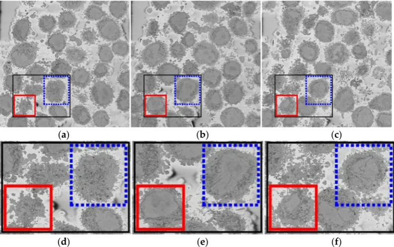
Figure 1. Three representative slices of a three-dimensional (3D) image stack acquired by Serial Block Face Scanning Electron Microscope (SBF SEM) containing numerous HeLa cells. Boxes indicate two regions of interest (ROIs), which contain two of the cells that will be posteriorly segmented. (a) A slice on the lower section of the stack; slice 43 of 300. (b) A slice on the central section; 118/300. (c) A slice on the higher section; 241/300. Black box denotes the ROI that is magnified in (d–f). Notice the differences in sizes of cell and nuclei in the images. In particular, the nuclei are hardly visible in (a), largest in (b), and in (c) the nucleus in the blue dotted box appears as several disjoint regions surrounded by a darker nuclear envelope (NE).

2.2. Ground Truth (GT)

Two cells (i.e., 600 slices) were manually segmented to provide a ground truth to assess the accuracy of the algorithm. Each cell was segmented by different persons without knowledge of each other and with different acquisition conditions. The first cell (shown by the red box in Figure 1) was segmented using Amira and a Wacom Cintiq 24HD interactive pen display by one of the authors (A.E.W.) and took around 30 hours. The second cell (shown by the blue box in Figure 1) was segmented by another author (C.K.) with a Wacom pen-and-tablet using the MATLAB® _{roipolyfunction and took}

around 47 hours. In both cases, in order to determine whether disjoint regions belong to the nucleus, the user scrolled up and down through neighbouring slices to check connectivity of the regions.

2.3. Automatic Segmentation of the Nuclear Envelope Algorithm

In this work, the NE of seven different cells were segmented and analysed. Intermediate steps of the segmentation algorithm consist of traditional image-processing steps: Low-pass filtering, edge detection, dilations, determination of superpixels, distance transforms, morphological operators, and post-processing to automatically segment the nuclear envelope (Figure 2). Images were initially

low-Figure 1.Three representative slices of a three-dimensional (3D) image stack acquired by Serial Block Face Scanning Electron Microscope (SBF SEM) containing numerous HeLa cells. Boxes indicate two regions of interest (ROIs), which contain two of the cells that will be posteriorly segmented. (a) A slice on the lower section of the stack; slice 43 of 300. (b) A slice on the central section; 118/300. (c) A slice on the higher section; 241/300. Black box denotes the ROI that is magnified in (d–f). Notice the differences in sizes of cell and nuclei in the images. In particular, the nuclei are hardly visible in (a), largest in (b), and in (c) the nucleus in the blue dotted box appears as several disjoint regions surrounded by a darker nuclear envelope (NE).

2.2. Ground Truth (GT)

J. Imaging2019,5, 75 5 of 17

2.3. Automatic Segmentation of the Nuclear Envelope Algorithm

In this work, the NE of seven different cells were segmented and analysed. Intermediate steps of the segmentation algorithm consist of traditional image-processing steps: Low-pass filtering, edge detection, dilations, determination of superpixels, distance transforms, morphological operators, and post-processing to automatically segment the nuclear envelope (Figure2). Images were initially low-pass filtered with a Gaussian kernel, with sizeh=7 and standard deviationσ=2, to remove high frequency noise. The algorithm exploited the abrupt change in intensity at the NE compared with the neighbouring cytoplasm and nucleoplasm by Canny edge detection [49]. The edges were dilated to connect disjoint edges by using the structural element of size 5 or greater than 5 depending on the standard deviation of the Canny edge detector. These disjoint edges were part of the NE and were initially missed due to intensity variations in the envelope itself (Figure2b). The connected pixels not covered by the dilated edges were labelled by the standard 8-connected objects found in the image to create a series of superpixels (Figure2c). We have dilated the same size as the width of the NE. The superpixel size was not restricted so that large superpixels covered the background and nucleoplasm. Morphological operators were used to remove regions in contact with the borders of the image, remove small regions, fill holes inside larger regions, and close the jagged edges (Figure2d).

J. Imaging 2019, 5, x FOR PEER REVIEW 5 of 16

pass filtered with a Gaussian kernel, with size h = 7 and standard deviation σ = 2, to remove high frequency noise. The algorithm exploited the abrupt change in intensity at the NE compared with the neighbouring cytoplasm and nucleoplasm by Canny edge detection [49]. The edges were dilated to connect disjoint edges by using the structural element of size 5 or greater than 5 depending on the standard deviation of the Canny edge detector. These disjoint edges were part of the NE and were initially missed due to intensity variations in the envelope itself (Figure 2b). The connected pixels not covered by the dilated edges were labelled by the standard 8-connected objects found in the image to create a series of superpixels (Figure 2c). We have dilated the same size as the width of the NE. The superpixel size was not restricted so that large superpixels covered the background and nucleoplasm. Morphological operators were used to remove regions in contact with the borders of the image, remove small regions, fill holes inside larger regions, and close the jagged edges (Figure 2d).

(a) (b) (c)

(d) (e) (f)

Figure 2. Intermediate steps of the segmentation algorithm. (a) Cropped region around one HeLa cell (dotted blue box in Figure 1c,f), surrounded by resin (background) and edges of other cells. This image was low-pass filtered. (b) Edges detected by Canny algorithm. The edges were further dilated to connect those edges that may belong to the nuclear envelope (NE) but were disjoint due to the variations of the intensity of the envelope itself. (c) Superpixels were generated by removing dilated edges. (d) Small superpixels and those in contact with the image boundary were discarded and the remaining superpixels were smoothed and filled, before discarding those by size that did not belong to the nucleus. (e) Final segmentation of the NE overlaid (thick black line) on the filtered image. (f) Ground truth (GT) manual segmentation of the same image. Regions not selected by the algorithm because of their sizes are highlighted with arrows. Notice that both the algorithm and GT detected disjoint regions.

A preliminary work approach described in [50] assumed that there was only one nuclear region in each image, which was designated as the nucleus, and any disjoint regions which could or not be part of the nucleus were ignored. That approach worked well for cells with a smooth near-spherical nuclear morphology. However, in cells with an irregular NE, disjoint regions were missed. To improve this approach, the new algorithm exploited the 3D nature of the data by using adjacent images to check for connectivity of islands to the main nuclear region, as a human operator would. It should be highlighted that the improvement is not only for small regions—these could be large. The original algorithm would only consider one region, and even if the second region would be close in

J. Imaging2019,5, 75 6 of 17

A preliminary work approach described in [50] assumed that there was only one nuclear region in each image, which was designated as the nucleus, and any disjoint regions which could or not be part of the nucleus were ignored. That approach worked well for cells with a smooth near-spherical nuclear morphology. However, in cells with an irregular NE, disjoint regions were missed. To improve this approach, the new algorithm exploited the 3D nature of the data by using adjacent images to check for connectivity of islands to the main nuclear region, as a human operator would. It should be highlighted that the improvement is not only for small regions—these could be large. The original algorithm would only consider one region, and even if the second region would be close in area to the first one, it would be discarded. The algorithm thus began at the central slice of the cell, which was assumed to be the one in which the nuclear region would be centrally positioned and have the largest diameter. The algorithm assumed that this slice would only have one nuclear region. The algorithm then proceeded in both directions (up and down through the neighbouring slices) and propagated the region labelled as nucleus to decide if a disjoint nuclear region in the neighbouring slices (above or below) was connected above or below the current slice of analysis (Figure3). When a segmented nuclear region overlapped with the previous nuclear segmentations, it was maintained; when there was no overlap, it was discarded.

By using neighbouring segmentations as input parameters to the current segmentation, and taking the regions into account, the algorithm was able to identify disjoint nuclear regions as part of a single nucleus (Figure2e). Finally, the NE was obtained as the boundary of the nucleus.

The algorithm was developed and validated on one cell (Figure4b), and tested on the NEs of the other six cells of which only one had a corresponding GT with 300 slices (Figure4d). All processing and visualisation was performed in MATLAB®(The MathworksTM, Natick, USA).

J. Imaging 2019, 5, x FOR PEER REVIEW 6 of 16

area to the first one, it would be discarded. The algorithm thus began at the central slice of the cell, which was assumed to be the one in which the nuclear region would be centrally positioned and have the largest diameter. The algorithm assumed that this slice would only have one nuclear region. The algorithm then proceeded in both directions (up and down through the neighbouring slices) and propagated the region labelled as nucleus to decide if a disjoint nuclear region in the neighbouring slices (above or below) was connected above or below the current slice of analysis (Figure 3). When a segmented nuclear region overlapped with the previous nuclear segmentations, it was maintained; when there was no overlap, it was discarded.

By using neighbouring segmentations as input parameters to the current segmentation, and taking the regions into account, the algorithm was able to identify disjoint nuclear regions as part of a single nucleus (Figure 2e). Finally, the NE was obtained as the boundary of the nucleus.

The algorithm was developed and validated on one cell (Figure 4b), and tested on the NEs of the other six cells of which only one had a corresponding GT with 300 slices (Figure 4d). All processing and visualisation was performed in MATLAB® _{(The Mathworks}TM_{, Natick, USA).}

Figure 3. Illustration of the propagation regions. Regions of a slice that overlap with the regions of a previous segmentation are maintained, whilst regions that do not are discarded. The algorithm propagates up and down, starting from central slice (slice number 150 for all seven cells which were segmented in this work), in the same way as a human expert to include or discard regions.

(a) (b)

J. Imaging2019,5, 75 7 of 17

J. Imaging 2019, 5, x FOR PEER REVIEW 6 of 16

area to the first one, it would be discarded. The algorithm thus began at the central slice of the cell, which was assumed to be the one in which the nuclear region would be centrally positioned and have the largest diameter. The algorithm assumed that this slice would only have one nuclear region. The algorithm then proceeded in both directions (up and down through the neighbouring slices) and propagated the region labelled as nucleus to decide if a disjoint nuclear region in the neighbouring slices (above or below) was connected above or below the current slice of analysis (Figure 3). When a segmented nuclear region overlapped with the previous nuclear segmentations, it was maintained; when there was no overlap, it was discarded.

By using neighbouring segmentations as input parameters to the current segmentation, and taking the regions into account, the algorithm was able to identify disjoint nuclear regions as part of a single nucleus (Figure 2e). Finally, the NE was obtained as the boundary of the nucleus.

The algorithm was developed and validated on one cell (Figure 4b), and tested on the NEs of the other six cells of which only one had a corresponding GT with 300 slices (Figure 4d). All processing and visualisation was performed in MATLAB® _{(The Mathworks}TM_{, Natick, USA).}

Figure 3. Illustration of the propagation regions. Regions of a slice that overlap with the regions of a previous segmentation are maintained, whilst regions that do not are discarded. The algorithm propagates up and down, starting from central slice (slice number 150 for all seven cells which were segmented in this work), in the same way as a human expert to include or discard regions.

(a) (b)

J. Imaging 2019, 5, x FOR PEER REVIEW 7 of 16

(c) (d)

Figure 4. Similarity metrics and final results of the automated segmentation displayed as rendered volumetric surfaces. (a) Jaccard Index (JI) (solid line) and Hausdorff distance (HD) (dotted line) for the segmented nuclear envelope (NE) shown in (b). Notice that the mean JI is 98% and the mean HD is 4 pixels for central slices. (b) Final result of the segmentation displayed as a rendered volumetric surface. The algorithm was developed and validated with this cell, and the arrow indicates an artefact due to a slight shift in the data during the image acquisition. The artefact was corrected with a pre-alignment. (c) JI and HD for the second NE shown in (d). Note the decrease in JI and increase in HD (arrows) towards the upper and lower edges of the NE, where the structure tends to become more fragmented in two-dimensional (2D) cross-sections and complex regions that may have been missed by the algorithm similar to those highlighted in Figure 2f.

2.4. Quantitative Comparisons

In order to assess the accuracy of the segmentation, the pixel-based metric Jaccard similarity index (JI) [52] was calculated. JI is also known as intersection over union. This metric is based on the determination of the true positives (TP, nuclear pixels segmented as nucleus), true negatives (TN, background pixels segmented as background), false positives (FP, background pixels segmented as nucleus), and false negatives (FN, nuclear pixels segmented as background), as illustrated in Figure 5 and defined by the following Equation:

Jaccard Similarity Index = (1)

(a) (b)

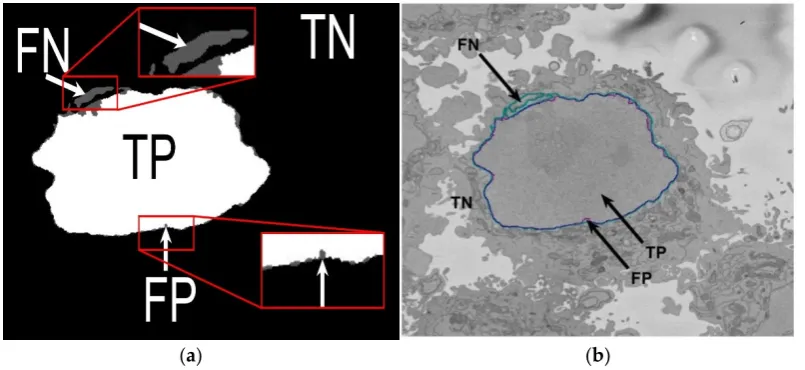
Figure 5. Illustration of the pixel-based metrics. (a) True Positives (TP, nuclear pixels segmented as nucleus), true negatives (TN, background pixels segmented as background), false positives (FP, background pixels segmented as nucleus), and false negatives (FN, nuclear pixels segmented as background). (b) Segmentation overlaid on one image: Ground truth (GT) in cyan, automated segmentation in purple.

Figure 4. Similarity metrics and final results of the automated segmentation displayed as rendered volumetric surfaces. (a) Jaccard Index (JI) (solid line) and Hausdorffdistance (HD) (dotted line) for the segmented nuclear envelope (NE) shown in (b). Notice that the mean JI is 98% and the mean HD is 4 pixels for central slices. (b) Final result of the segmentation displayed as a rendered volumetric surface. The algorithm was developed and validated with this cell, and the arrow indicates an artefact due to a slight shift in the data during the image acquisition. The artefact was corrected with a pre-alignment. (c) JI and HD for the second NE shown in (d). Note the decrease in JI and increase in HD (arrows) towards the upper and lower edges of the NE, where the structure tends to become more fragmented in two-dimensional (2D) cross-sections and complex regions that may have been missed by the algorithm similar to those highlighted in Figure2f.

2.4. Quantitative Comparisons

In order to assess the accuracy of the segmentation, the pixel-based metric Jaccard similarity index (JI) [52] was calculated. JI is also known as intersection over union. This metric is based on the determination of the true positives (TP, nuclear pixels segmented as nucleus), true negatives (TN, background pixels segmented as background), false positives (FP, background pixels segmented as nucleus), and false negatives (FN, nuclear pixels segmented as background), as illustrated in Figure5 and defined by the following Equation:

Jaccard Similarity Index = TP

J. Imaging2019,5, 75 8 of 17

J. Imaging 2019, 5, x FOR PEER REVIEW 7 of 16

(c) (d)

Figure 4. Similarity metrics and final results of the automated segmentation displayed as rendered volumetric surfaces. (a) Jaccard Index (JI) (solid line) and Hausdorff distance (HD) (dotted line) for the segmented nuclear envelope (NE) shown in (b). Notice that the mean JI is 98% and the mean HD is 4 pixels for central slices. (b) Final result of the segmentation displayed as a rendered volumetric surface. The algorithm was developed and validated with this cell, and the arrow indicates an artefact due to a slight shift in the data during the image acquisition. The artefact was corrected with a pre-alignment. (c) JI and HD for the second NE shown in (d). Note the decrease in JI and increase in HD (arrows) towards the upper and lower edges of the NE, where the structure tends to become more fragmented in two-dimensional (2D) cross-sections and complex regions that may have been missed by the algorithm similar to those highlighted in Figure 2f.

2.4. Quantitative Comparisons

In order to assess the accuracy of the segmentation, the pixel-based metric Jaccard similarity index (JI) [52] was calculated. JI is also known as intersection over union. This metric is based on the determination of the true positives (TP, nuclear pixels segmented as nucleus), true negatives (TN, background pixels segmented as background), false positives (FP, background pixels segmented as nucleus), and false negatives (FN, nuclear pixels segmented as background), as illustrated in Figure 5 and defined by the following Equation:

Jaccard Similarity Index = (1)

(a) (b)

Figure 5. Illustration of the pixel-based metrics. (a) True Positives (TP, nuclear pixels segmented as nucleus), true negatives (TN, background pixels segmented as background), false positives (FP, background pixels segmented as nucleus), and false negatives (FN, nuclear pixels segmented as background). (b) Segmentation overlaid on one image: Ground truth (GT) in cyan, automated segmentation in purple.

Figure 5. Illustration of the pixel-based metrics. (a) True Positives (TP, nuclear pixels segmented as nucleus), true negatives (TN, background pixels segmented as background), false positives (FP, background pixels segmented as nucleus), and false negatives (FN, nuclear pixels segmented as background). (b) Segmentation overlaid on one image: Ground truth (GT) in cyan, automated segmentation in purple.

In addition, the Hausdorffdistance (HD) of the maximum of the set of shortest distances between two curves was calculated to assess how far the real boundary of the NE was from the segmented NE.

HD [53] is defined as the maximum distance between a point on one curve and its nearest neighbour on the other curve [54,55] and defined by the following Equation:

dH(A,B) =max (

sup in f d(a,b), sup in f d(a,b) a∈_{A b}∈_{B b}∈_{B a}∈_A

)

(2)

In both cases, the metrics (JI, HD) were calculated on a per-slice basis. JI is a strict measurement as compared with accuracy and other metrics, as it does not include the true negatives. On the other hand, accuracy includes the TN in both numerator and denominator and this, especially in cases where the objects of interest are small and there are large areas of background (e.g., the upper and lower slices of the cell), would render very high accuracy. As JI does not count TN, the values decrease towards the higher and lower slices of the cells, as can be seen in the edges of Figure4a,c. Accuracy values would increase in these slices.

2.5. Active Contours

J. Imaging2019,5, 75 9 of 17

J. Imaging 2019, 5, x FOR PEER REVIEW 8 of 16

In addition, the Hausdorff distance (HD) of the maximum of the set of shortest distances between two curves was calculated to assess how far the real boundary of the NE was from the segmented NE.

HD [53] is defined as the maximum distance between a point on one curve and its nearest neighbour on the other curve [54,55] and defined by the following Equation:

𝑑 𝐴, 𝐵

𝑚𝑎𝑥 𝑠𝑢𝑝 𝑖𝑛𝑓 𝑑 𝑎, 𝑏 , 𝑠𝑢𝑝 𝑖𝑛𝑓 𝑑 𝑎, 𝑏

𝑎 ∈ 𝐴 𝑏 ∈ 𝐵 𝑏 ∈ 𝐵 𝑎 ∈ 𝐴

In both cases, the metrics (JI, HD) were calculated on a per-slice basis. JI is a strict measurement as compared with accuracy and other metrics, as it does not include the true negatives. On the other hand, accuracy includes the TN in both numerator and denominator and this, especially in cases where the objects of interest are small and there are large areas of background (e.g., the upper and lower slices of the cell), would render very high accuracy. As JI does not count TN, the values decrease towards the higher and lower slices of the cells, as can be seen in the edges of Figure 4a,c. Accuracy values would increase in these slices.

2.5. Active Contours

In order to compare the algorithm segmentation with an alternative approach, the NE was segmented with Chan–Vese active contours methodology [56] (Figure 6). The function changes its parameters based on one of three states: Shrink, Grow, or Normal. One of the three states and its parameters were chosen empirically through numerous tests. A small circle was placed in the middle of the HeLa nucleus in one of the 300 images (Red box in Figure 1b) with the help of the MATLAB®

roipoly function and allowed to grow for a number of iterations. The number of iterations was increased in steps of 100 with the objective of determining the optimum number, i.e., to obtain the highest JI, and to continue until the algorithm had segmented not just the NE, but the whole cell. Practically, this consisted of running the algorithm up to 5000 iterations. In total, 50 out of 300 slices were segmented by the same method, and both JI and HD were computed. They were compared with the algorithm segmentation metrics. The parameters were adjusted (contraction bias = −0.4, smooth factor = 1.5, iterations = 5000) and the active contours was run again to obtain foreground and background.

(a) (b) (c) (d)

(e) (f) (g) (h)

Figure 6. Comparison of the algorithm against ground truth (GT) and Active Contours. (a) One representative slice from one HeLa cell (red box in Figure 1b). Green dashed-dotted box denotes the region of interest (ROI) that is magnified in (e–h). (b) Automated segmentation of the nuclear envelope (NE) (purple). For comparison, the hand segmented GT is shown (cyan). (c) Active contours segmentation with 2200 iterations provided the highest Jaccard index (JI) 75%. (d) Active contours

Figure 6. Comparison of the algorithm against ground truth (GT) and Active Contours. (a) One representative slice from one HeLa cell (red box in Figure1b). Green dashed-dotted box denotes the region of interest (ROI) that is magnified in (e–h). (b) Automated segmentation of the nuclear envelope (NE) (purple). For comparison, the hand segmented GT is shown (cyan). (c) Active contours segmentation with 2200 iterations provided the highest Jaccard index (JI) 75%. (d) Active contours segmentation with 5000 iterations included large sections of the cell showing the influence of the iterations on the result.

Shrink and Normal, the other two states of active contours, were also implemented but the best result was obtained by the state of Grow.

2.6. Nuclear Envelope Shape Modelling

In order to further study the shape of the segmented NE, this was modelled against a spheroid. The spheroid was created with the same volume as the nucleus and the position adjusted to fill the NE as closely as possible, as illustrated in Figure7a, where NE is displayed as a red rendered volumetric surface and the spheroid as blue mesh

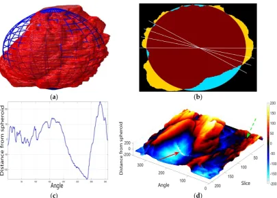
The surfaces of the spheroid and the nucleus were subsequently compared by tracing rays (Figure7b) from the centre of the spheroid and the distance between the surfaces for each ray was calculated (Figure 7c). It was designated that when the NE was further away from the centre, the difference was positive. Figure7d shows the surface corresponding to the distance from the NE of the first cell (Figure4b) to a model spheroid. The notch that travels along the cell between slices is visible (red arrow) and the dashed green arrow highlights a particularly rugged region (Figure7d). It should be noted that this process is automatic without any user intervention. In order to position the spheroid, the centroid of the segmented cell was calculated, and the coordinates were used as the centre of the spheroid.

J. Imaging2019,5, 75 10 of 17

J. Imaging 2019, 5, x FOR PEER REVIEW 9 of 16

segmentation with 5000 iterations included large sections of the cell showing the influence of the iterations on the result.

Shrink and Normal, the other two states of active contours, were also implemented but the best result was obtained by the state of Grow.

2.6. Nuclear Envelope Shape Modelling

In order to further study the shape of the segmented NE, this was modelled against a spheroid. The spheroid was created with the same volume as the nucleus and the position adjusted to fill the NE as closely as possible, as illustrated in Figure 7a, where NE is displayed as a red rendered volumetric surface and the spheroid as blue mesh

The surfaces of the spheroid and the nucleus were subsequently compared by tracing rays (Figure 7b) from the centre of the spheroid and the distance between the surfaces for each ray was calculated (Figure 7c). It was designated that when the NE was further away from the centre, the difference was positive. Figure 7d shows the surface corresponding to the distance from the NE of the first cell (Figure 4b) to a model spheroid. The notch that travels along the cell between slices is visible (red arrow) and the dashed green arrow highlights a particularly rugged region (Figure 7d). It should be noted that this process is automatic without any user intervention. In order to position the spheroid, the centroid of the segmented cell was calculated, and the coordinates were used as the centre of the spheroid.

(a) (b)

(c) (d)

Figure 7. Nuclear envelope (NE) surface modelling against a spheroid. (a) Rendering of the nuclear envelope (NE) (red surface) against the model spheroid (blue mesh). (b) Illustration of distance calculations by ray tracing in one slice. Yellow regions correspond to the nucleus outside the spheroid, cyan regions to nucleus inside the spheroid. (c) Measurements obtained along the boundary. (d) Surface corresponding to the distance from the NE to a model spheroid. Solid red arrow indicates a notch, dashed green arrow shows rugged region.

Numerous metrics that characterise the NE can now be extracted, either directly from the NE: nuclear volume, Jaccard Index (JI) to the spheroid, or from the altitudes of the modelled surface: (mean value (μ) and standard deviation (σ)), range of altitudes. Other derived metrics can also be

Figure 7.Nuclear envelope (NE) surface modelling against a spheroid. (a) Rendering of the nuclear envelope (NE) (red surface) against the model spheroid (blue mesh). (b) Illustration of distance calculations by ray tracing in one slice. Yellow regions correspond to the nucleus outside the spheroid, cyan regions to nucleus inside the spheroid. (c) Measurements obtained along the boundary. (d) Surface corresponding to the distance from the NE to a model spheroid. Solid red arrow indicates a notch, dashed green arrow shows rugged region.

3. Results and Discussion

The algorithm was designed and trained on one cell from which the parameters were derived. The algorithm was then applied to seven cells from which the nuclear envelope was segmented (Figure4b,d and Figure8(Left)) with accurate results for the two sets for which 300 slices of ground truth were available and good visual assessment of the remaining five. The shapes of the final segmentations show the complexity of the NE with rather convoluted notches and invaginations. It is speculated that these shapes may have biological significance which is beyond the scope of this paper.

J. Imaging2019,5, 75 11 of 17

J. Imaging 2019, 5, x FOR PEER REVIEW 11 of 16

Figure 8. Final results of the automated segmentation displayed as rendered volumetric surfaces and modelling for six cells. Left: Segmentation results displayed as rendered volumetric surfaces for six different cells. In each cell, note the notches and invaginations, which may be relevant biological characteristics of the cells. Right: Surfaces corresponding to the distance from the nuclear envelope (NE) to a model spheroid. Arrows, in the last four rows, show notches that travel along the nuclei (grey, yellow, purple, and cyan cell).

Table 1 illustrates the previously described metrics that can be extracted from the NE and the surface. Mean (μ), standard deviation (σ), and range of values, which are related to the height of

J. Imaging2019,5, 75 12 of 17

The automated segmentations were compared to manual GT segmentations in order to assess the accuracy of the algorithm. Two different similarity metrics, JI and HD, were computed. For the cell shown in Figure4b (red cell), all 300 slices were visually checked and it was noticed that the bottom 26 and top 40 slices did not contain any cell—therefore, they were not included in similarity metrics calculations. The algorithm detected cells in all slices between 42 and 254, and JI and HD were computed as 93% and 9 pixels, respectively. For the slices between 50 and 250, the mean JI is 95% and the mean HD 8, and for slices between 75 and 225 (interquartile range, IQR), the mean JI is 98% with the mean HD 4 pixels (Figure4a). Similarly, the bottom 40 of 300 slices of the cell shown in Figure4d showed no cell 259 and the algorithm detected the cell for all slices between 47 and 289, and JI and HD were computed as 90% and 17 pixels, respectively. The mean JI is 93% and the mean HD 13 pixels for slices between 50 and 250, and 94% with the mean HD 13 pixels for slices between 75 and 225 (Figure4c). JI decreased and HD increased towards the top and bottom of the cells, as the structure was considerably more complex and the areas become much smaller (Figure4a,c).

Active contours, on the other hand, provided much lower values of JI with a highest value of 75% (illustrated on slice 118/300—Figure6c,d), and took considerably longer, as 2200 iterations required 27 minutes for one slice only. In total, 50 out of 300 slices were segmented by active contours in 31 h. On the other hand, the algorithm described segmented each slice in ~8 s and the whole cell in approximately 40 min; that is, the segmentation of two slices with active contours would take longer than the algorithm for 300 slices.

The comparison between the model spheroid and the whole nucleus (shown in Figure4b) reported a JI of 66% (Figure7). Notice that in this case, JI is measuring how spherical the NE is, not the accuracy of the segmentation. This value indicates a relative departure from a spheroid and it is speculated that the JI could be related to biological characteristics of cells. In addition, the measurements of distance from the nucleus to the spheroid showed rougher and smoother regions (Figure7a,b,d). The surface corresponding to the distance from the nuclear envelope to a model spheroid (Figure7d) showed graphically the hollow and prominent regions of the cell, but more important, elements such as a notch (solid red arrow) or ruggedness (dashed green arrow) can be an indication of NE breaking down or remodelling. An advantage of this modelling is that visually it is easier to assess a single 2D image than a 3D volumetric surface, as can be seen in Figure8where six cells and their corresponding surfaces are shown. Mercator map projection was used in this modelling against a spheroid and this could be a limitation of the algorithm. Whilst there are many interesting characteristics such a large notch on the NE of the third (grey) cell or large protuberance on the second (green) cell, at this moment it is only possible to speculate the biological correlation between the surfaces and the nature of the cell itself.

Table1illustrates the previously described metrics that can be extracted from the NE and the surface. Mean (µ), standard deviation (σ), and range of values, which are related to the height of peaks and depth of valleys, could be related to some biological state of the cells; however, this has not yet been verified.