Novel algorithms for 3D surface point cloud boundary detection and edge reconstruction

(1)

Novel algorithms for 3D surface point cloud boundary detection

and edge reconstruction

Carmelo Mineo

⇑

, Stephen Gareth Pierce, Rahul Summan

Department of Electronic and Electrical Engineering, University of Strathclyde, Royal College Building, 204 George Street, Glasgow G1 1XW, UK

a r t i c l e i n f o

Article history:

Received 20 October 2017

Received in revised form 5 February 2018 Accepted 6 February 2018

Available online 7 February 2018

Keywords: Point-cloud Boundary detection Edge reconstruction

a b s t r a c t

Tessellated surfaces generated from point clouds typically show inaccurate and jagged boundaries. This can lead to tolerance errors and problems such as machine judder if the model is used for ongoing man-ufacturing applications. This paper introduces a novel boundary point detection algorithm and spatial FFT-based filtering approach, which together allow for direct generation of low noise tessellated surfaces from point cloud data, which are not based on pre-defined threshold values. Existing detection tech-niques are optimized to detect points belonging to sharp edges and creases. The new algorithm is tar-geted at the detection of boundary points and it is able to do this better than the existing methods. The FFT-based edge reconstruction eliminates the problem of defining a specific polynomial function order for optimum polynomial curve fitting. The algorithms were tested to analyse the results and mea-sure the execution time for point clouds generated from laser scanned meamea-surements on a turbofan engine turbine blade with varying numbers of member points. The reconstructed edges fit the boundary points with an improvement factor of 4.7 over a standard polynomial fitting approach. Furthermore, through adding artificial noise it has been demonstrated that the detection algorithm is very robust for out-of-plane noise lower than 25% of the cloud resolution and it can produce satisfactory results when the noise is lower than 75%.

Ó2018 Society for Computational Design and Engineering. Publishing Services by Elsevier. This is an open access article under the CC BY-NC-ND license (http://creativecommons.org/licenses/by-nc-nd/4.0/).

1. Introduction

Three-dimensional (3D) scanning is increasingly used to anal-yse objects or environments in diverse applications including industrial design, orthotics and prosthetics, gaming and film pro-duction, reverse engineering and prototyping, quality control and documentation of cultural and architectural artefacts (Curless,

1999; Levoy & Whitted, 1985). Conventional reconstruction

tech-niques generate tessellated surfaces from point clouds. Such tessel-lated models often show inaccurate and jagged boundaries that can lead to tolerance errors and problems such as machine judder if the models are used for ongoing manufacturing applications

(Beard, 1997). That is the reason why many existing commercial

computer-aided manufacturing (CAM) applications are not able to use tessellated models, instead of using precise analytical CAD models where the surfaces are mathematically represented

(Mineo, Pierce, Nicholson, & Cooper, 2017). Whilst the conversion

of analytical geometries into meshed surfaces is straightforward,

the reverse process of conversion of a tessellated model into an analytical CAD model is challenging and time-consuming. There are circumstances where the original CAD model of a component is not available or deviates from the real part. New CAM software applications, able to use clean tessellated models, are emerging

(Mineo et al., 2017); they enable the direct use of triangulated

point clouds obtainable through surface mapping techniques. However, the point clouds obtained through surface mapping are typically affected by noise. New algorithms for optimum surface mesh refinement are required to improve the performance of emerging applications and to overcome the limitations of typical approaches based on polynomial smoothing. Different technolo-gies can be used to build coordinate measuring machines (CMM) or 3D-scanning devices (Curless, 1999). Each technology comes with its own limitations, advantages and costs. A common factor for many CMM and 3D scanners is that they can measure the coor-dinates of a large number of points on an object surface and output a point cloud of the scanned area. However, point clouds are gen-erally not directly usable in most 3D applications, and therefore are usually converted to mesh models, NURBS surface models, or CAD models (Berger et al., 2017; Hinks, Carr, Truong-Hong, & Laefer,

2012; Truong-Hong, Laefer, Hinks, & Carr, 2011). Tessellated

mod-els have emerged as a favoured technique; they are the easiest

https://doi.org/10.1016/j.jcde.2018.02.001

2288-4300/Ó2018 Society for Computational Design and Engineering. Publishing Services by Elsevier. This is an open access article under the CC BY-NC-ND license (http://creativecommons.org/licenses/by-nc-nd/4.0/). Peer review under responsibility of Society for Computational Design and

Engineering.

⇑ Corresponding author.

E-mail address:[email protected](C. Mineo).

Contents lists available atScienceDirect

Journal of Computational Design and Engineering

(2)

form of virtual models obtainable from point clouds with minimal processing. There are two different approaches to create a triangu-lar meshed surface from a point cloud: using triangulation meth-ods or surface reconstruction methmeth-ods. Triangulation algorithms use the original points of the input point cloud, using them as the vertices of the mesh triangles. The Delaunay triangulation, named after Boris Delaunay for his work on the topic from 1934

(Delaunay, 1934), is the most popular algorithm of this kind. A

bi-dimensional Delaunay triangulation ensures that the circumcir-cle associated with each triangle contains no other point in its inte-rior. This definition extends naturally to three dimensions considering spheres instead of circles. Surface reconstruction algo-rithms differ from the triangulation method since they do not use the original points as the vertices of the mesh triangles but com-pute new points, whose density can vary according to the local cur-vature of the 3D geometry. Surface reconstruction from oriented points can be cast as a spatial problem, based on the Poisson’s equation (Calakli & Taubin, 2011; Kazhdan & Hoppe, 2013).

Both approaches are not able to reconstruct the surface bound-aries accurately, which makes the tessellated models unsuitable to be used for CAM toolpath generation. Triangulation methods pro-duce meshed surfaces with jagged boundaries since the original noisy points of the cloud are used as vertices of the mesh triangles. Reconstruction methods produce smooth boundaries, but they can be quite far from the original boundaries of the real surface. Indeed, Poisson’s surface reconstruction does not follow the boundary of the point cloud and replaces the original points with new points laying on a reconstructed continuous surface that sat-isfies the Poisson’s differential equation.

The detection of cloud boundary points and the reconstruction of smooth boundary edges would allow trimming of the recon-structed tessellated models, to refine the mesh boundaries. Very few feature detection methods are optimized to work with point-sampled geometries only. The major problem of these point based methods is the lack of knowledge concerning point normal and connectivity. This makes feature detection a more challenging task

than in mesh-based methods. Gumhold, Wang, and MacLeod

(2001)presented an algorithm that first analyses the

neighbour-hood of each point via a principal component analysis (PCA). The eigenvalues of the correlation matrix are then used to determine if a point belongs to a feature. This technique for the detection of features in point clouds is used as a pre-processing step for tessel-lated surface reconstruction with sharp features (Weber,

Hahmann, & Hagen, 2011). There exist also several reconstruction

methods that preserve sharp features during the surface recon-struction of a point cloud without pre-processing; for example, the methods shown by Fleishman, Cohen-Or, and Silva (2005)

andÖztireli, Guennebaud, and Gross (2009).

The existing techniques mentioned above are optimized to detect points belonging to sharp edges. This paper presents novel algorithms targeted to the detection of boundary points and the deterministic reconstruction of accurate and smooth surface boundaries from 3D point clouds. A smart approach known as Mesh Following Technique (MFT) (Mineo et al., 2017), for the gen-eration of robot tool-paths from STL models, has recently been published. The technique requires virtual tessellated surfaces with smooth boundary edges.

The algorithms presented in this paper are useful tools to refine the boundary of tessellated surfaces obtained from 3D scanning point cloud data. They can be used to trim Delaunay triangulation or Poisson’s reconstructed surface meshes, facilitating the direct use of tessellated models, instead of analytical geometries. The remainder part of the paper describes the algorithms and shows qualitative and quantitative results, discussing advantages and disadvantages.

2. Detection of boundary points

Given a mapped surface in the form of a point cloud, the iden-tification of the point cloud borderline, thus the detection of boundary points, is not a trivial task. The human brain is able to infer the border of a point cloud by simply looking at the arrange-ment of the sparse points. In computer science and computational geometry, a point cloud is an entity without a well-defined bound-ary. In the bi-dimensional domain, given a finite set of points, the problem of detecting the smallest convex polygon that contains all the given points of the cloud is solved through the quickhull

method (Barber, Dobkin, & Huhdanpaa, 1996). It uses a divide and conquer approach. This method works well but is only able to detect the boundary points that are part of the convex polygon and is only for a set of points. A generalization ofquickhull, able to handle concave regions and holes in the point cloud, is the alpha-shapeapproach (Akkiraju et al., 1995). The Computational Geome-try Algorithms Library (CGAL) (Kettner, Näher, Goodman and

O’Rourke 2004) has a robust implementation of alpha-shape for

that produces a satisfactory result for a point cloud may not be suitable for other point sets since point clouds can exhibit different point densities. This inconve-nience is similar to what happens when obtaining a black and white picture from a grayscale image, through thresholding the pixel intensities; the optimal threshold value is affected by the average brightness of the image. Moreover, when the point density of a point cloud varies between across the cloud, the alpha-shape result can be satisfactory in some regions and poor in others. Non-parametric edge extraction methods based on kernel regres-sion (Öztireli et al., 2009) and on analysis of eigenvalues

(Bazazian, Casas, & Ruiz-Hidalgo, 2015) have been proposed in

recent years. Such methods, however, are optimized for the detec-tion of internal sharp edges, rather than detecting the point cloud borderline.

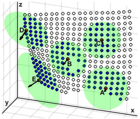
The boundary point detection algorithm presented in this paper, herein referred as BPD algorithm, does not need the defini-tion of any threshold values. For every region of the cloud, it detects as many boundary points as possible, given the local reso-lution of the region. A 3D-point cloud is unorganized and the neighbourhood of a point is more complex than that of a pixel in an image. Generally, in 3D-point clouds, there are three types of neighbourhoods: spherical neighbourhood, cylindrical

neighbour-hood, and k-nearest neighbours based neighbourhood

(Weinmann, Jutzi, Hinz, & Mallet, 2015). The three types of

(3)

circles. The semi-transparent circles, centred at the points from A to E, highlight the best fit planes for each of the neighbourhoods. The normal directions of such planes are also shown through arrows pointing outwards from the neighbourhood parent points. The local cloud resolution for every member of the cloud is esti-mated through the following steps. Given a point of the cloudPi, for every point of its neighbourhood (Pi;j), the minimum distance (dj;k) between that point and all other neighbours is computed. The local point cloud resolution (bi) in Pi is estimated as

a

is set too low. On the other hand, it may detect unwanted bound-ary points, if

a

is too high. The new method described here is cap-able of detecting boundary points belonging to convex and concave regions.

The BPD method exploits the fact that there is one and only one circle that passes through three given points in the 3D space. Given the unclassified pointPi, the centre and the radius of all circles that pass forPiand any two other points of its neighbourhood are com-puted. The point is labelled as a boundary point if there is at least one circle with radius equal or bigger thanbiand if the sphere for

Pi, whose centre coincides with the centre of the circle, does not contain any other point of the neighbourhood. This is the case for point A and B, shown inFig. 1. Point A and B are two boundary points, since it is possible to find at least one circle that satisfies the above conditions (Fig. 2). In order to avoid unnecessary compu-tational efforts and yet consider all possible circles, all the originat-ing point triples are identified through the binomial coefficient

(Biggs, 1979). Working with k-nearest neighbourhoods and being

the investigated pointPi always part of the triples, the remaining points (k-1) are combined in couples with no repetitions. Thus, the total number of circles is equal to:

n¼ ðk1Þ! 2! ½ðk1Þ 2!¼

29! 227!¼

2928

2 ¼406 ð1Þ

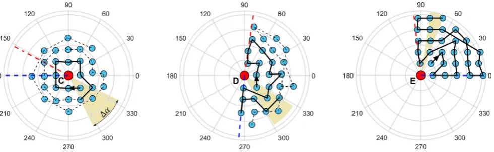
Although the presence of at least one circle that satisfies the above conditions allows to classify the investigated point as belonging to the point cloud boundary, its absence cannot be used to state that the point is an internal point of the cloud. Indeed the investigated point Pi can be located on a convex region of the boundary as well as being an internal point of the cloud. In such circumstances, although it may exist one circle with radius equal or bigger thanbi, the sphere for Pi, centred at the centre of the cir-cle, will always contain some points of the neighbourhood. This is the case for the points C, D and E shown inFig. 1. For such kind of points, thus when the point cannot be labelled as a boundary point through the first part of the detection algorithm described above, the algorithm continues with further operations. Each investigated point and its neighbours are projected to the best fit plane accord-ing to the normal vector associated with the point. The resultaccord-ing bi-dimensional neighbourhood cloud can be plotted in polar coor-dinates, with Piat the pole of the plot.Fig. 3shows the polar plots for point C, D and E and their neighbours. Piis shown in red and its neighbour points are shown in blue. The blue and red dotted line of the plots inFig. 3highlight, respectively, the minimum and maxi-mum angle of the angular sector spanned by the points in the neighbourhood.

The fundamental idea behind the final step of the BPD algo-rithm is that the point of the cloud Piis a boundary point if it is not possible to find a path that surrounds it and passes through the neighbour points. Each point on the polar plot is determined by the distance from the pole (radial coordinate,R) and the angular coordinate (h). Given a neighbourhood, the developed algorithm creates a path that surrounds the parent point at the pole. An incre-mental approach is used. All radial and angular coordinates of the neighbours are normalized so that the coordinates of the j-th neighbour point are:

rj¼

RjRmin

RmaxRmin ð2Þ

#j¼ hjhmin

hmaxhmin ð3Þ

[image:3.595.51.286.65.264.2]

Fig. 2.A and B labelled as boundary points.

p

. In summary, the BPD method described here is capable of determining if a point Pibelongs to a concave boundary section (e.g. point A inFig. 1) when the local curvature is as high as 1=bi. The method is also able to infer if a point belongs to the boundary of a hole in the point cloud (e.g. point B inFig. 1) when the hole radius is as small asbi. Sincebiis the local resolution, the method works well on point clouds with variable point density.

3. Edge reconstruction

The application of the BPD algorithm to the point cloud sample shown inFig. 1finds all the boundary points, represented as empty circles inFig. 4. Also, the 4 boundary points of the internal circular hole, whose radius is just above the local point cloud resolution, are detected as expected. The detected points need to be clustered so that points belonging to the same boundary are grouped together. Moreover, the points of every cluster need to be ordered correctly. These tasks can be fulfilled through existing algorithms. For example, the clustered points can be ordered through algo-rithms capable of solving the so-calledtravelling salesman problem

(TSP). Given a random list of points and the distances between each pair of points, the solution of the TSP is the shortest possible path that crosses each point exactly once and returns to the origin point (Schrijver, 2005). Therefore a closed boundary path is obtained from every cluster. These boundaries, given by the ordered points linked through line segments (see dashed lines in

Fig. 4) can be quite jagged in some areas. Therefore, it is evident

[image:4.595.53.544.66.217.2]

that such boundaries are not suitable to trim the surface meshes obtainable from the point cloud. The boundary curves need smoothing to better resemble the real surface borderlines. This section of the paper introduces a novel raw boundary smoothing algorithm, herein referred as RBS algorithm, to improve the recon-struction of surface point cloud borderlines through accurate smoothing of the raw boundaries.

[image:4.595.312.544.536.721.2]

Fig. 3.Polar plot of point C, D and E and their neighbours. The solid and dashed lines illustrate the application of the algorithm.

(5)

3.1. Detection of key points

Before applying any smoothing algorithm to the closed loop boundary curves, it is necessary to highlight that the position of some of the detected boundary points should be preserved. This is the case for the borderline corners, where there is a sharp change in the boundary directionality. Indeed, such points usually play a crucial role in the definition of reference systems in CAM applica-tions for the development of accurate operaapplica-tions, where the cor-rect registration of the part virtual model is required. Therefore, the first step of the edge reconstruction algorithm is targeted to detect such key points. Given the i-th point of a closed boundary path, the point is labelled as corner if the radius of the circle for the investigated point, the precedent and the successive point is smaller than the value of the local point cloud resolution,bi(as cal-culated in the detection algorithm). This approach is able to iden-tify the corner points fromP1toP5, highlighted with asterisks in

Fig. 4. It is worth noticing here that, although the corners can be

found through applying a threshold value to the angle between the two borderline segments for each investigated point (Ni, Lin,

Ning, & Zhang, 2016), this approach is advantageous and it is

suit-able to work with point clouds with varisuit-able density. The identified corners are used to divide the closed loop boundary into sections, corresponding to the edges of the surface geometry. The external boundary points of the cloud inFig. 4 are grouped in 5 edges. The 4 internal boundary points are grouped in one single closed loop edge since no corners are found there.

3.2. Limitation of traditional curve smoothing methods

Each edge could be smoothed through fitting a polynomial curve. Polynomial curve fitting is a common smoothing method and the functionality is also implemented in CAD/CAM commercial software applications (e.g. RhinocerosÒ). Curve fitting is the pro-cess of approximating a pattern of points with a mathematical function (Arlinghaus, 1994). Fitted curves can be used to infer the values of a function where no data are available (Johnson &

Williams, 1976) (e.g. in the gaps between sampled points). The

goal of curve fitting is to model the expected value of a dependent variableyin terms of the value of an independent variable (or vec-tor of independent variables)x. In general, the expected value ofy

can be modelled as an nth_{degree polynomial function, yielding the} general polynomial regression model based on the truncated Tay-lor’s series:

y¼a0þa1xþa2x2þ. . .þanxnþ

e

ð6Þ

where

e

is a random error with null mean. Given the points of an edge and the order of the target polynomial function, it is possible to compute the coefficients of the fitting function. The limitation of this smoothing approach is that the order of the target function is typically unknown and curve fitting remains a time-consuming iterative trial and error process for edge reconstruction. When there is no theoretical basis for choosing the order of the fitting polyno-mial function, the edges may be fitted with a spline function com-posed of a sum of B-splines (Knott, 2012). The places where the B-splines meet are known as knots. The main difficulty in applying this process is in determining the number of knots to use and where they should be placed (de Boor, 1968).

3.3. FFT-based reconstruction

The final step of the RBS algorithm, presented in this paper, introduces a robust approach based on the Fast Fourier Transform (FFT). The FFT is a well-known way to translate the information contained in a waveform from the time domain to frequency

domain. It is used for the spectral analysis of time-series and allows the application of high or low-pass filters, to respectively attenuate low or high frequencies. Here the FFT is applied to the pattern of the edge point Cartesian coordinates, to enable the application of low-pass filters able to improve the smoothness of the boundary edges. The exploitation of FFT to spatial patterns (waveforms sampled in the Cartesian domain rather than the time domain) is not new (e.g. it has been used for image processing)

(Gonzales & Woods, 1992). However, there is no record of the

FFT being applied to the problem of surface edge reconstruction. The nuances of the adaptation of FFT to this problem are described herein.

p

bi: ð7Þ

The smallest edge radius of curvature that is possible to recon-struct at the i-th point will be equal toRmax

i ¼bi.

(6)

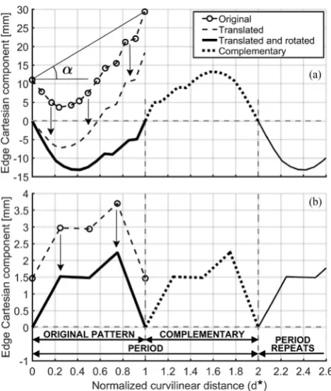
a complementary portion creating a period with the translated and rotated version of the original pattern (Fig. 5a). Since the FFT assumes a constant sampling rate of the input pattern, the original randomly spaced samples are replaced with interpolated equally spaced samples. The number of interpolated samples (Np) is chosen appropriately to give a constant sampling interval (dsÞ, equal or smaller than the minimum original sampling distance. In order to ensure a good filtering performance, it is necessary to have suf-ficient spatial frequency resolution. For such reason the period is repeated to get a minimum of 1000 samples in the input waveform of the FFT, giving a frequency resolution of fs¼1=ð1000dsÞ. Therefore a low-pass filter is applied, cancelling all spatial fre-quency components higher thanfmax, as expressed in Eq.(7). This produces a smoothed waveform for the edge component. The FFT input waveform shown inFig. 5a, artificially constructed to filter the x-component of the open edge comprised betweenP2andP3, has a null mean value. The original edge extremities lie on the hor-izontal axis (the mean value line) and are not affected by the low-pass filtering. The Cartesian component values of the extremities are preserved. The first part of the waveform (the portion up to the total lengthDof the original pattern) is rotated by negative

a

and translated back to the original position. The smoothed bound-ary is obtained through filtering all the Cartesian components of all its edges. The preservation of the original edge extremity points makes sure that, when a boundary consists of multiple edges, two consecutive edges share a common point. Therefore, the chain of edges forms a closed boundary. If a boundary is formed by only one closed edge, like in the case of the internal hole boundary in

Fig. 4, the extremities of each of its Cartesian components have

the same value (

a

¼0). Moreover, the complementary portion to construct the period is a mere horizontally translated copy of the Cartesian component pattern (after its extremities are brought to the horizontal axis). The copy of the original pattern is not inverted nor flipped to create the complementary portion (Fig. 5b). All points of the closed edge are affected by the filtering. The

smoothed edges relative to the boundaries of the sample point cloud are shown through solid line curves inFig. 4.

4. Results and performances

This section of the paper analyses the results obtainable through the use of the introduced BPD and RBS algorithms. The computational performances are also examined and quantitative figures are reported.Fig. 6shows a schematic summary of the algo-rithm steps. The thick dashed line perimeters contain the novel algorithm components introduced by this paper. The BPD algo-rithm (Fig. 6a) allows the unlabelled point of a surface point cloud to be grouped into two groups: boundary points and internal points. The boundary points are clustered and ordered, through existing algorithms, to constitute raw closed boundaries (jagged). The RBS algorithm (Fig. 6b) identifies the boundary corners and divides each closed boundary into the constituting edges. Every edge is smoothed through spatial FFT-based filtering. A crucial advantage of the introduced algorithms is that they are not based on any threshold values that can be suitable for some point cloud but not suitable for others. The BPD is capable of labelling all points, observing the local resolution of the cloud for each point. The FFT-based edge reconstruction eliminates the problem of defining a specific polynomial function order for optimum polyno-mial curve fitting. In the approach introduced in this paper, the best edge smoothing performance is also ensured through applying a spatial low-pass filtering with a frequency defined at every boundary point as a function of the local cloud resolution.

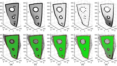
In order to show the potentialities of the new algorithms, an air-craft turbine engine fan blade, 640 mm long and 300 mm wide (in average) was scanned through a coordinate measuring machine. The FARO Quantum Arm was used in conjunction with a laser pro-file mapping probe (Monchalin, Neron, Bouchard, & Heon, 1998). This 3D scanning equipment has a volumetric maximum deviation of ±74

l

m. The blade surface was scanned to obtain a uniform point cloud with circa 14 thousand points (approximately 72 points per square centimetre).

The cloud points were decimated to obtain four different point cloud versions, with target resolution respectively equal to 4, 8, 16 and 34 mm. An additional point cloud was generated with variable point resolution, between 2 and 34 mm. Such generated point clouds allowed testing the algorithms under controlled situations and facilitated the analysis of the results. In order to introduce well-defined internal boundaries, the points found within three spheres centred at fixed positions and with radii equal to 16, 32 and 64 mm were removed from the clouds. Therefore, each cloud presents three holes (H1, H2, and H3), with radii approximatively equal to the original generating spheres. The resulting five point clouds are shown by the top row plots inFig. 7. These plots show the detected boundary points through darker round point marks. The external and internal boundary points are detected as expected. The smallest radius of the hole detectable in a point cloud depends on the cloud resolution, as described in Section2. Only four points of the 16 mm and 32 mm radius holes (H1 and H2) are detected in the clouds ofFig. 7c and7d, since the resolution of these clouds is close to their radii. H1 cannot be detected on the 34 mm resolution cloud (Fig. 7d).

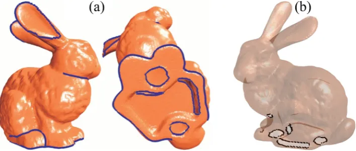
Fig. 8 shows the boundary points detected in the Stanford

bunny (Turk & Levoy, 1994a), an open source computer graphics test meshed model, obtained through range scanning (Turk &

Levoy, 1994b). Similarly to how many researchers have used this

[image:6.595.40.275.64.341.2]

model, as input for surface reconstruction algorithms, the mesh connectivity has been stripped away and the vertices have been treated as an unorganized point cloud in this work. It presents 35,947 points and has an average resolution of 1.2 mm. Boundary

(7)

[image:7.595.54.552.64.407.2]

Fig. 6.Schematic summary of the algorithm steps: boundary point detection (a) and edge reconstruction (b).

[image:7.595.56.552.449.732.2]

(8)

points were detected using a method based on principal compo-nent analysis (PCA) (Gumhold et al., 2001) (Fig. 8a) and the new detection algorithm (Fig. 8b). To appreciate the differences in per-formance it is important to differentiate boundary points and edge points; the latter points are located in areas where there is a sharp ripple (like in the bunny ears). The PCA method detected points that are either on sharp crease lines or on the borderline of the point cloud holes. The BPD algorithm is targeted to exclusively find borderline points; therefore it found two holes on the base of the bunny, originating from the original clay model (it was a hollow model). It should be noted that the BPD algorithm should not detect the extra edge and crease points detected by PCA (e.g. in the ears of the bunny). It is designed to detect boundary points (around holes or areas where the point density drops drastically), so that a boundary edge can be reconstructed and the tessellated surface can be trimmed. The BPD algorithm was capable of detect-ing four additional groups of boundary points (one group under the bunny chest, one group between the bunny front legs and two groups on the base), corresponding to the borderline of areas with poor range scanning coverage. The smallest two of these areas were not detected by the PCA method, showing how the BPD algo-rithm is more accurate for the detection of borderline points.

The bottom row plots ofFig. 7shows the reconstructed bound-ary edges. The effectiveness of the FFT-based filtering algorithm is evident observing the smoothness of the edges. The smoothed boundaries of the internal holes, given by single closed edges, faithfully reproduces the roundness of the theoretical intersection between the original generating sphere and the blade surface. Only the boundaries of H1 and H2, reconstructed through only four detected points, show visible distortion. Although explaining how mesh trimming works is out of the scope of this paper, the recon-structed boundary edges can be used to trim the Poisson mesh, producing the clean boundary meshes highlighted inFig. 7.

The algorithms were tested, using a computing machine based on an IntelÒCore(TM) i7-6820HQ CPU (2.70 GHz), with 32 Gb of RAM. The tests were carried out through MATLABÒ2016a, running on the Windows 10 64-bit operating system.Table 1reports quan-titative outcomes obtained from the application of the BPD algo-rithm to the point clouds given inFig. 7. The initial rows of the table report the minimum, the mean, the maximum cloud resolu-tion (_b) and its standard deviation (

r

), followed by the number of points in the clouds. Therefore the table gives the number of boundary points detected by the detection algorithm and the time taken (in milliseconds [ms]) for its complete execution. The elapsed time is always lower than 3 s for all examined point clouds.

[image:8.595.116.470.67.217.2]

The point clouds obtained through some 3D scanning methods are affected by out-of-plane noise, meaning that the sampled points deviate from their ideal version lying on the surface. It is important to estimate how much the proposed detection algorithm is tolerant to such noise. Therefore the detection algorithm was repeatedly applied to versions of the point clouds with increasing random noise added to the original points. The noisy clouds were artificially obtained by moving each point along the normal direc-tion of the local k-neighbourhood best fit plane. Each point was moved by distances equal to a percentage of the local cloud reso-lution. Starting from 0%, the noise percentage was increased by 1% at every repetition of the detection algorithm. The maximum percentage value after which at least one of the boundary points is not detected (false negative) is denoted asX. The value ofXis around 25% for all the clouds ofFig. 7. If the noise percentage is increased above X, some internal points of the cloud may be labelled as boundary points (false positives). The maximum per-centage value after which at least one of the internal points is labelled as boundary point is denoted asW. The values of Win

Table 1are all above 75%. Therefore, the detection algorithm is very

[image:8.595.33.550.657.752.2]

Fig. 8.Detected points on the Stanford bunny (Turk & Levoy, 1994a), with a method based on principal component analysis (Gumhold et al., 2001) (a) and with the BPD algorithm (b).

Table 1

Performances obtained from the application of the BPD algorithm.

Cloud a b c d e

Minb[mm] 3.82 7.77 15.53 32.29 1.98

Meanb[mm] 4.19 8.44 16.87 34.52 3.71

Maxb[mm] 4.85 9.36 18.98 40.42 34.86

SD (r) [mm] 0.11 0.20 0.52 1.14 4.30

Number of points 12,309 3095 791 203 7458

Boundary points 632 315 156 72 397

Detection time [ms] 2606 944 340 289 1892

X[% ofbi] 25% 24% 27% 25% 26%

(9)

robust for out-of-plane noise lower than 25% of the cloud resolu-tion and it can produce satisfactory results when the noise is lower than circa 75%. With noise values between 25% and 75% of the cloud resolution, the detection algorithm will miss some boundary points but no outliers will be generated.

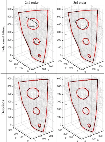
Fig. 9compares, for the 16 mm average resolution point cloud,

polynomial fitting and B-spline edges of 2nd and 3rd order with the edges reconstructed through the new RBS approach (as described within the thickest dashed perimeter inFig. 6b). It is evi-dent that the polynomial fitting produces unsatisfactory edges, especially for the internal boundaries. B-spline edges present excessive wrinkling, thus poor smoothing.

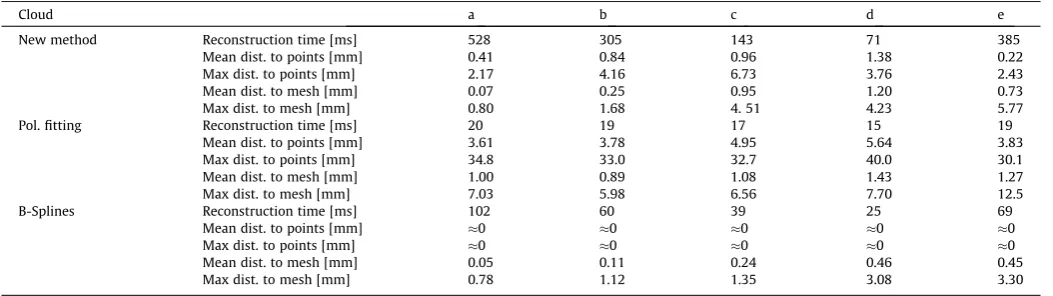
Table 2gives quantitative results on the performance of the RBS

algorithm, compared to 3rd order polynomial fitting and B-splines, for all point clouds inFig. 7.

[image:9.595.123.483.248.735.2]

Although the execution time of the new FFT-based algorithm is always one order of magnitude higher than the time for polynomial fitting and for B-spline computation, the smooth edges produced by the new approach fit the surface contour better than polynomial fitting and B-splines. The table reports the mean, max-imum and standard deviation (STD) values for the distances between the boundary points and the smoothed edges and for the distance between the reconstructed surface mesh and the reconstructed edges. In average, the reconstructed edges computed through the new approach fit the boundary points 4.7 times better than the 3rd order polynomial edges. Moreover, they follow the reconstructed surface mesh contour 77% better than the polynomial fitting edges. Although the B-splines seem to follow the reconstructed mesh better than the new approach, 3rd order B-splines do not produce significant smoothing of the

(10)

original boundary points; the distance between the B-splines and the points being circa equal to 0 is not a sign of good performance. The accuracy with which the polynomial and B-spline edges fit the boundary points and the reconstructed surface can be improved by increasing the order of the functions, but this impacts on the time required to compute the function coefficients. Moreover, high order polynomials often suffer from severe ringing between the data points. The RBS approach reconstructs the optimum edges without the need to specify any parameter, unlike the function order in the polynomial and the B-spline fitting.

5. Conclusions

Tessellated surfaces generated from point clouds typically show inaccurate and jagged boundaries. This can lead to tolerance errors and problems such as machine judder if the model is used for ongoing manufacturing applications. This is the reason why many existing commercial computer-aided manufacturing (CAM) appli-cations are not able to use tessellated models. This work presented novel algorithms to refine the boundary of meshed surfaces obtained from 3D scanning point cloud data. The BPD algorithm allows the unlabelled point of a surface point cloud to be grouped into two groups: boundary points and internal points. Existing detection techniques are optimized to detect points belonging to sharp edges and creases. The BPD algorithm is targeted to the detection of boundary points and it is able to do this better than the existing methods. The RBS algorithm identifies the boundary corners and divides each closed boundary into the constituting edges. Every edge is smoothed through spatial FFT-based filtering. A crucial advantage of the introduced algorithms is that they are not based on any threshold values that can be suitable for some point cloud but not suitable for others. The FFT-based edge recon-struction eliminates the problem of defining a specific polynomial function order for optimum polynomial curve fitting. The algo-rithms were tested to analyse the results and measure the execu-tion time for point clouds generated from laser scanned measurements on a turbofan engine turbine blade with varying numbers of member points. Through adding artificial noise it has been demonstrated that the BPD algorithm is very robust for out-of-plane noise lower than 25% of the cloud resolution and it can produce satisfactory results when the noise is lower than circa 75%. With noise values between 25% and 75% of the cloud resolu-tion, the detection algorithm will miss some boundary points but no outliers will be generated. Quantitative results on the perfor-mance of the RBS algorithm were also presented. The recon-structed edges computed through the new approach fit the

boundary points by a factor of 4.7 times better than polynomial edges. Moreover, they follow the reconstructed surface mesh con-tour with an improvement of 77% compared to the polynomial fit-ting edges.

Acknowledgements

This work is part of the Autonomous Inspection in Manufactur-ing and Re-ManufacturManufactur-ing (AIMaReM) project, funded by the UK Engineering and Physical Science Research Council (EPSRC) through the grant EP/N018427/1. The authors also wish to thank Dr. Maxim Morozov for acquiring the point cloud of the turbofan engine turbine blade considered in this paper.

Appendix A. Supplementary material

Supplementary data associated with this article can be found, in the online version, athttps://doi.org/10.1016/j.jcde.2018.02.001.

References

Akkiraju, N., Edelsbrunner, H., Facello, M., Fu, P., Mücke, E., Varela, C. (1995). Alpha shapes: Definition and software. In Proceedings of the 1st international computational geometry software workshop(p. 66)

Arlinghaus, S. (1994).Practical handbook of curve fitting. CRC Press.

Barber, C. B., Dobkin, D. P., & Huhdanpaa, H. (1996). The quickhull algorithm for convex hulls.ACM Transactions on Mathematical Software (TOMS), 22, 469–483. Bazazian, D., Casas, J. R., Ruiz-Hidalgo, J. (2015). Fast and robust edge extraction in unorganized point clouds. In: International conference on digital image computing: Techniques and applications (DICTA)(pp. 1–8).

Beard, T. (1997). Machining from STL files.Modern Machine Shop, 69, 90–99. Berger, M., Tagliasacchi, A., Seversky, L. M., Alliez, P., Guennebaud, G., Levine, J. A.,

et al. (2017). A survey of surface reconstruction from point clouds.Computer Graphics Forum, 301–329.

Biggs, N. L. (1979). The roots of combinatorics.Historia Mathematica, 6, 109–136. Calakli, F., & Taubin, G. (2011). SSD: Smooth signed distance surface reconstruction.

Computer Graphics Forum, 1993–2002.

Curless, B. (1999). From range scans to 3D models.ACM SIGGRAPH Computer Graphics, 33, 38–41.

de Boor, C. (1968). On the convergence of odd-degree spline interpolation.Journal of Approximation Theory, 1, 452–463.

Delaunay, B. (1934). ‘‘Sur la sphere vide,” Izv. Akad. Nauk SSSR, Otdelenie Matematicheskii i Estestvennyka Nauk(Vol. 7, pp. 1–2).

Fleishman, S., Cohen-Or, D. & Silva, C. T. (2005). Robust moving least-squares fitting with sharp features. In ACM transactions on graphics (TOG), (Vol. 0, pp. 544– 552).

Gonzales, R. C., & Woods, R. E. (1992).Digital image processing. Reading, MA: Addison & Wesley Publishing Company.

Gumhold, S., Wang, X., & MacLeod, R. S. (2001). Feature Extraction From Point Clouds. InIMR.

Hinks, T., Carr, H., Truong-Hong, L., & Laefer, D. F. (2012). Point cloud data conversion into solid models via point-based voxelization.Journal of Surveying Engineering, 139, 72–83.

[image:10.595.32.559.86.234.2]

Johnson, D., & Williams, R. P. D. (1976). Methods of experimental physics: Spectroscopy. New York: Academic Press.

Table 2

Performances of the RBS algorithm, compared to 3rd order polynomial fitting.

Cloud a b c d e

New method Reconstruction time [ms] 528 305 143 71 385

Mean dist. to points [mm] 0.41 0.84 0.96 1.38 0.22

Max dist. to points [mm] 2.17 4.16 6.73 3.76 2.43

Mean dist. to mesh [mm] 0.07 0.25 0.95 1.20 0.73

Max dist. to mesh [mm] 0.80 1.68 4. 51 4.23 5.77

Pol. fitting Reconstruction time [ms] 20 19 17 15 19

Mean dist. to points [mm] 3.61 3.78 4.95 5.64 3.83

Max dist. to points [mm] 34.8 33.0 32.7 40.0 30.1

Max dist. to mesh [mm] 7.03 5.98 6.56 7.70 12.5

B-Splines Reconstruction time [ms] 102 60 39 25 69

Mean dist. to points [mm] 0 0 0 0 0

Max dist. to points [mm] 0 0 0 0 0

(11)

Kazhdan, M., & Hoppe, H. (2013). Screened Poisson surface reconstruction.ACM Transactions on Graphics (TOG), 32, 29.

Kettner, L., Näher, S., Goodman, J. E., & O’Rourke, J. (2004). Two computational geometry libraries: LEDA and CGAL. InHandbook of discrete and computational geometry(pp. 1435–1463). Chapman & Hall/CRC.

Knott, G. D. (2012).Interpolating cubic splines(Vol. 18). Springer Science & Business Media.

Levoy, M., & Whitted, T. (1985).The use of points as a display primitive. University of North Carolina, Department of Computer Science.

Mineo, C., Pierce, S. G., Nicholson, P. I., & Cooper, I. (2017). Introducing a novel mesh following technique for approximation-free robotic tool path trajectories. Journal of Computational Design and Engineering, 4(3), 192–202.

Monchalin, J.-P., Neron, C., Bouchard, P., & Heon, R. (1998). Laser-ultrasonics for inspection and characterization of aeronautic materials. Journal of Nondestructive Testing & Ultrasonics (Germany), 3, 002.

Ni, H., Lin, X., Ning, X., & Zhang, J. (2016). Edge detection and feature line tracing in 3d-point clouds by analyzing geometric properties of neighborhoods.Remote Sensing, 8, 710.

Öztireli, A. C., Guennebaud, G., & Gross, M. (2009). Feature preserving point set surfaces based on non-linear kernel regression. Computer Graphics Forum, 493–501.

Schrijver, A. (2005). On the history of combinatorial optimization (till 1960). Handbooks in Operations Research and Management Science, 12, 1–68. Truong-Hong, L., Laefer, D. F., Hinks, T., & Carr, H. (2011). Flying voxel method with

Delaunay triangulation criterion for façade/feature detection for computation. Journal of Computing in Civil Engineering, 26, 691–707.

Turk, G. & Levoy, M. (1994). The Stanford bunny, the Stanford 3D scanning repository.

Turk G, & Levoy, M. (1994). Zippered polygon meshes from range images. In: Proceedings of the 21st annual conference on Computer graphics and interactive techniques(pp. 311–318).

Weber, C., Hahmann, S. & Hagen, H. (2011). Methods for feature detection in point clouds. InOASIcs-OpenAccess Series in Informatics.