City, University of London Institutional Repository
Citation
:
Guo, Z., Ma, Q. ORCID: 0000-0001-5579-6454 and Qin, H. (2018). A novel 2.5D method for solving the mixed boundary value problem of a surface effect ship. Applied Ocean Research, 78, pp. 25-32. doi: 10.1016/j.apor.2018.05.016This is the accepted version of the paper.
This version of the publication may differ from the final published
version.
Permanent repository link: http://openaccess.city.ac.uk/20253/
Link to published version
:
http://dx.doi.org/10.1016/j.apor.2018.05.016Copyright and reuse:
City Research Online aims to make research
outputs of City, University of London available to a wider audience.
Copyright and Moral Rights remain with the author(s) and/or copyright
holders. URLs from City Research Online may be freely distributed and
linked to.
City Research Online: http://openaccess.city.ac.uk/ [email protected]
1
A novel 2.5D method for solving the mixed boundary value problem
of a surface effect ship
Zhiqun Guo1, Q.W. Ma2,1,*, Hongde Qin1
1
College of Shipbuilding Engineering, Harbin Engineering University
2
School of Engineering and Mathematical Sciences, City University London
* Correspondence: [email protected]
Abstract: When a surface effect ship (SES) sails in waves, the unsteady velocity potential of water can be decomposed into incident potential, sidehull radiation potential, sidehull diffraction potential and radiation
potential due to fluctuating air pressure. The potentials related to sidehulls satisfy Neumann boundary conditions
(BC) and have been successfully addressed using the 2.5D method. In contrast, the potential related to fluctuating air pressure satisfies mixed BC consisting of homogeneous Neumann BC on the wetted surface of
sidehulls and nonhomogeneous Dirichlet BC on the interface between air and water, which has never been studied using the efficient 2.5D method. In this paper, the 2.5D method is firstly proposed to solve the mixed boundary value problem (BVP), which can deal with the coupling between the fluctuating air pressure and sidehulls. By using the 2.5D method, the radiation wave and other relative hydrodynamic parameters of a SES due to the fluctuating air pressure are evaluated. The numerical results on motion response and the fluctuated air pressure of the SES show acceptable agreement with the experimental ones.
Keywords: 2.5D method; mixed boundary value problem; surface effect ship; air cushion
1. Introduction
The surface effect ship (SES) is a kind of high speed vessel widely used in the marine transportation. When
navigating in waves, the SES makes unsteady motions, and the pressure in the air cushion fluctuating due to the pumping effect of waves. Inversely, the unsteady motions of sidehulls and the fluctuating air pressure can have
influence on the motion of water, which induce the sidehull radiation potential, sidehull diffraction potential and radiation potential due to fluctuating air pressure. One needs to solve all of these velocity potentials for reckoning the responses of the SES in waves.
The sidehull radiation and diffraction potentials satisfy nonhomogeneous Neumann boundary condition (BC)
on the wetted surface of sidehulls and homogeneous Dirichlet BC on the interface between air cushion and water.
The latter is actually similar to the conventional free surface condition, which makes the sidehull radiation and diffraction potentials obtained by simply solving Neumann boundary value problems (BVP). In this sense, the hydrodynamics of the SES sidehulls is the same as conventional catamarans. 3D numerical methods such as Rankine source method (Connell et al., 2011), finite element method (García-Espinosa et al., 2015) and URANS
method (Bhushan et al., 2017) have been employed in literature to precisely evaluate the hydrodynamics of SES sidehulls. However, the 3D methods are computationally expensive and might not meet the engineering demands.
2
efficiency of the methods. To enhance the computational efficiency, Guo et al. (2015) employed the 2.5D method to calculate the hydrodynamic coefficients of a special SES, which is called Partial Air Cushion Supported
Catamaran (PACSCAT). The 2.5D method is very efficient because the free surface condition in it is kept
three-dimensional, while the governing equations and body surface conditions are reduced to two-dimensional (Faltinsen and Zhao, 1991; Ma et al., 2005).
On the other hand, the radiation potential due to fluctuating air pressure satisfies the mixed BC consisting of
homogeneous Neumann BC and nonhomogeneous Dirichlet BC, the latter of which is built through the Bernoulli’s
equation. To obtain the radiation potential due to fluctuating air pressure, one has to solve the mixed BVP. The 3D numerical methods can be utilized to do so, but they still consume a significant amount of computational resources. For the sake of simplicity, in some works (Doctors, 1976; Xie et al., 2008) the mixed BVP was
simplified to a Dirichlet BVP, i.e. the homogeneous Neumann BC as well as the coupling between the fluctuating
air pressure and sidehulls was neglected. The simplification, however, inevitably has impact on the numerical
precision and thus one cannot obtain the accurate radiation potential due to fluctuating air pressure.
A possible approach to overcome the aforementioned difficulties is to exploit the2.5D method to solve the mixed BVP, which has advantages of accuracy and efficiency. However, the 2.5D method generally was exploited to solve the Neumann BVP (Faltinsen and Zhao, 1991; Ma et al., 2005; Guo et al., 2015), i.e. hydrodynamic problems of displacement or planing ships, or the Dirichlet BVP (Guo et al., 2017), i.e.
hydrodynamic problems of hovercrafts, and has never been employed to solve the mixed BVP.
In this paper, the2.5D method is firstly employed to solve the mixed BVP arising from the unsteady motions of a SES. By using the 2.5D method, we solve the radiation potential due to fluctuating air pressure, as well as the radiation waves on the interface and radiation forces on the wetted surface of sidehulls. The obtained results are
substituted into the motion equations of a PACSCAT to find the motion response and the fluctuating air pressure in the air cushion. The numerical results are compared with the experimental data in a few cases. The object of the present paper is to provide an efficient and accurate method to evaluate the hydrodynamics of air cushion in a SES.
2. Mathematical model of the mixed BVP and corresponding 2.5D numerical method
Let 𝑂 − 𝑋𝑌𝑍 be an earth-fixed coordinate system and 𝑜 − 𝑥𝑦𝑧 a SES-accompanied coordinate system.
The latter is always parallel to 𝑂 − 𝑋𝑌𝑍. When the SES is at its mean position, the 𝑥-axis is pointing upstream parallel to the longitudinal plane of the SES and the 𝑧-axis is pointing vertically upward through the center of
gravity (COG) of the SES. The origins of both coordinate systems are located in the plane of mean free surface.
2.1. Governing equations for hydrodynamics of the SES
Let 𝛷I= 𝜂0𝜙Iei𝜔𝑡 be the incident wave, where 𝜂0 is the wave amplitude, 𝜙I the spatial component of
𝛷I with an unit amplitude, 𝜔 the encountered frequency. Within the framework of linear assumption, the
unsteady disturbed velocity potential around the SES can be written as
𝜙T= 𝜙D+ 𝜙R+ 𝜙P= {𝜂0𝜙0+ ∑6𝑗=1𝜂𝑗𝜙𝑗+ ∑6+𝑁𝑗=7P𝜂𝑗𝜙𝑗}ei𝜔𝑡 (1)
where 𝜙D, 𝜙R, 𝜙P are sidehull diffraction potential, sidehull radiation potential and radiation potential due to
3
the incident wave, 𝜙𝑗(𝑗 = 1, … ,6) the spatial component of 𝜙R in 𝑗-th motion mode of an unit amplitude,
𝜙𝑗(𝑗 = 7, … ,6 + 𝑁P) the spatial component of 𝜙P in 𝑗-th mode, 𝜂𝑗 (𝑗 = 1, … ,6) the amplitude of 𝑗-th motion
mode, 𝜂𝑗(𝑗 = 7, … ,6 + 𝑁P) the equivalent waterhead of the fluctuating air pressure in 𝑗-th mode, 𝑁P the
number of modes.
The fluctuating air cushion pressure on the interface can be expressed as
𝑝̃(𝑥, 𝑦, 𝑡) = 𝑝̂(𝑥, 𝑦)ei𝜔𝑡= −ρwgei𝜔𝑡∑6+𝑁𝑗=7P𝜂𝑗𝑁𝑗(𝑥, 𝑦) (2)
where 𝑝̂(𝑥, 𝑦) is the spatial component of 𝑝̃(𝑥, 𝑦, 𝑡), ρw the density of water, g the gravity, 𝑁𝑗(𝑥, 𝑦) a
complete set of orthogonal Fourier modes expanded on the interface defined as (Lee and Newman, 2015)
𝑁𝑗(𝑥, 𝑦)= (
cos(𝛼π(𝑥 − 𝑥m) 𝑙⁄ )
sin(𝛼π(𝑥 − 𝑥m) 𝑙⁄ )) (
cos(𝛽π𝑦 𝑏⁄ )
sin(𝛽π𝑦 𝑏⁄ )) (3)
where 𝛼, 𝛽 are even for the modes corresponding to the cosine or odd for the sine; 𝑙, 𝑏, 𝑥m are the length,
breadth, and longitudinal center of the air cushion, respectively.
According to the Bernoulli’s equation, the boundary condition on the interface between water and air is
∑ 𝜂𝑗((i𝜔 − 𝑈 𝜕 𝜕𝑥)
2
+ g𝜕𝑧𝜕) 𝜙𝑗 6+𝑁P
𝑗=7 = g ∑ 𝜂𝑗(i𝜔 − 𝑈
𝜕
𝜕𝑥)𝑁𝑗(𝑥, 𝑦) 6+𝑁P
𝑗=7 (4)
where 𝑈 is the forward speed of the SES.
If the sidehulls of the SES are slender and the forward speed is high (the Brard number 𝑈𝜔/g is farlarger than 0.25 (Ma et al., 2005)), the high-speed slender body assumption could be applied to the sidehulls of the SES, under which the surge potential 𝜙1 is neglected. Then the BVP for the sidehull radiation and diffraction
potentials (𝜙𝑗, 𝑗 = 0,2, … ,6) can be formulated as
{
∂2𝜙 𝑗
∂𝑦2 +
∂2𝜙 𝑗
∂𝑧2 = 0, in 𝛺
[(i𝜔 − 𝑈 𝜕
𝜕𝑥) 2
+ g 𝜕
𝜕𝑧] 𝜙𝑗= 0, on 𝑆F∪ 𝑆P 𝜕𝜙𝑗
𝜕𝑛 = {
i𝜔𝑛𝑗+ 𝑈𝑚𝑗, 𝑗 = 2, … ,6
−𝜕𝜙I
𝜕𝑛 , 𝑗 = 0
, on 𝑆B
𝜙𝑗 = 𝜕𝜙𝑗
𝜕𝑥 = 0, at 𝑥 > 𝑥0
𝜙𝑗 = ∇𝜙𝑗= 0, on 𝑆∞
(5)
where 𝛺, 𝑆B, 𝑆P, 𝑆F, 𝑆∞ are the fluid domain enclosed by the mean wetted body surface 𝑆P, the mean interface 𝑆P between air cushion and water, the mean free surface 𝑆F, the boundary 𝑆∞ at infinity; 𝑥0 is the
𝑥-coordinate of the bow; 𝑛𝑗(𝑗 = 1, … ,6) is the generalized normal vector, and 𝑚𝑗 is defined as
(𝑚1, 𝑚2, 𝑚3) = (0,0,0) and (𝑚4, 𝑚5, 𝑚6) = (0, 𝑛3, −𝑛2).
Analogously, if the air cushion is slender (the ratio of the length to beam 𝑙 𝑏⁄ is larger than 2 (Guo et al., 2017)) and the forward speed is high (the Froude number 𝐹𝑟𝑙 is larger than 0.4 (Guo et al., 2017)), the
4 {
∂2𝜙 𝑗
∂𝑦2 +
∂2𝜙 𝑗
∂𝑧2 = 0, in 𝛺
((i𝜔 − 𝑈 𝜕
𝜕𝑥) 2
+ g𝜕
𝜕𝑧) 𝜙𝑗 = {
g (i𝜔 − 𝑈𝜕𝑥𝜕)𝑁𝑗(𝑥, 𝑦)
0, ,
on 𝑆P
on 𝑆F 𝜕𝜙𝑗
𝜕𝑛 = 0, on 𝑆B
𝜙𝑗 = 𝜕𝜙𝑗
𝜕𝑥 = 0, at 𝑥 > 𝑥0
𝜙𝑗 = ∇𝜙𝑗= 0, on 𝑆∞
(6)
The mixed BVP (6) is a novel model presented in this work, in which the sidehull effects on the velocity potential due to pressure are firstly considered. In contrast, in previous papers (Xie et al., 2008; Guo et al., 2015) the sidehull effects were ignored. Obviously, Eq.(5) and Eq.(6) are Neumann BVP and mixed BVP, respectively. The Neumann BVP (5) has be successfully solved using the 2.5D method (Ma et al., 2005), while the mixed BVP (6) has never been tried using the 2.5D method.
2.2. The mixed BVP solved using the 2.5D method
The 2.5D method resolves a 3D frequency-domain BVP by converting it into one defined in a 2D
time-domain. To do so, the following variable substitutions need to be made
{
𝑥(𝑡) = 𝑥0− 𝑈𝑡
𝜓𝑗(𝑡, 𝑦, 𝑧) = ei𝜔𝑡𝜙𝑗(𝑥(𝑡), 𝑦, 𝑧)
𝛱𝑗(𝑡, 𝑦) = ei𝜔𝑡𝑁𝑗(𝑥(𝑡), 𝑦)
(7)
Substituting Eq.(7) into the 3D frequency-domain BVP (6) yields a 2D time-domain BVP
{
∂2𝜓𝑗
∂𝑦2 +
∂2𝜓𝑗
∂𝑧2 = 0, in 𝛺
𝜕2𝜓 𝑗
𝜕𝑡2 + g
𝜕𝜓𝑗
𝜕𝑧 = {
g𝜕𝛱𝜕𝑡𝑗 0, ,
on 𝑆P
on 𝑆F 𝜕𝜓𝑗
𝜕𝑛 = 0, on 𝑆B
𝜓𝑗= 0, 𝑡 ≤ 0
𝜕𝜓𝑗
𝜕𝑡 = {
g𝛱𝑗(0, 𝑦),
0,
𝑡 = 0, on 𝑆P
𝑡 = 0, on 𝑆F
𝜓𝑗= ∇𝜓𝑗 = 0, on 𝑆∞
(8)
The 2D time-domain free surface Green’s function is proposed to solve the time-domain mixed BVP (8):
𝐺(𝒑, 𝑡; 𝒒, 𝜏) = 𝛿(𝑡 − 𝜏)ln𝑟𝑟𝑝𝑞
𝑝𝑞̅− 𝐻(𝑡 − 𝜏)𝐺̃(𝒑, 𝑡; 𝒒, 𝜏) (9)
𝐺̃(𝒑, 𝑡; 𝒒, 𝜏) = 2 ∫ √g 𝑘∞ ⁄ e𝑘(𝑧+𝜁)cos(𝑘(𝑦 − 𝜂)) sin (√g𝑘(𝑡 − 𝜏)) d𝑘
0 (10)
where 𝒑, 𝒒 and 𝒒̅ are the field point, source point andthe mirror of source point about the mean free surface, respectively; 𝑟𝑝𝑞and 𝑟𝑝𝑞̅ are the distance from 𝒑 to 𝒒 and from 𝒑 to 𝒒̅, respectively; 𝛿(∙) and 𝐻(∙) are
Dirac and Heaviside functions, respectively; 𝐺̃ is the free surface memory term of the Green’s function.
Applying the Green’s theorem to 𝜓𝑗(𝜏, 𝒒) and 𝐺̃(𝒑, 𝑡; 𝒒, 𝜏), one gets
∫ (𝜓𝑗
𝜕𝐺̃ 𝜕𝑛𝑞− 𝐺̃
𝜕𝜓𝑗
𝜕𝑛𝑞) d𝑠𝑞
5
It is well known that the integral on 𝑆∞ in Eq.(11) is equals to 0. Considering this and integratingEq.(11) over
𝜏 yields
∫ d𝜏 ∫ (𝜓𝑗 𝜕𝐺̃ 𝜕𝑛𝑞− 𝐺̃
𝜕𝜓𝑗
𝜕𝑛𝑞) d𝑠𝑞
𝑆F+𝑆B+𝑆P
𝑡
0 = 0 (12)
Using the free surface condition, the integral on 𝑆P in Eq.(12) comes to
∫ d𝜏 ∫ (𝜓𝑗 𝜕𝐺̃ 𝜕𝑛𝑞− 𝐺̃
𝜕𝜓𝑗
𝜕𝑛𝑞) d𝑠𝑞
𝑆P
𝑡
0 = ∫ 𝜓𝑗
𝜕 𝜕𝜁ln
𝑟𝑝𝑞
𝑟𝑝𝑞̅d𝑠𝑞
𝑆P + ∫ d𝜏 ∫ 𝛱𝑗(𝜏, 𝜂)
𝜕𝐺̃ 𝜕𝜏d𝑠𝑞 𝑆P
𝑡
0 (13)
Analogously, using the interface condition, the integral on 𝑆F reads
∫ d𝜏 ∫ (𝜓𝑗 𝜕𝐺̃ 𝜕𝑛𝑞− 𝐺̃
𝜕𝜓𝑗
𝜕𝑛𝑞) d𝑠𝑞
𝑆F
𝑡
0 = ∫ 𝜓𝑗
𝜕 𝜕𝜁ln
𝑟𝑝𝑞
𝑟𝑝𝑞̅d𝑠𝑞
𝑆F (14)
On the other hand, applying Green’s theorem to 𝜓𝑗(𝜏, 𝒒) and ln 𝑟𝑝𝑞
𝑟𝑝𝑞̅, one obtains
2π𝜓𝑗(𝑡, 𝒑) − ∫ (𝜓𝑗(𝑡, 𝒒) 𝜕 𝜕𝑛𝑞ln
𝑟𝑝𝑞
𝑟𝑝𝑞̅− ln
𝑟𝑝𝑞
𝑟𝑝𝑞̅
𝜕𝜓𝑗(𝑡,𝒒)
𝜕𝑛𝑞 ) d𝑠𝑞
𝑆B
= ∫ 𝜓𝑗(𝑡, 𝒒) 𝜕 𝜕𝜁ln
𝑟𝑝𝑞
𝑟𝑝𝑞̅d𝑠𝑞+ ∫ 𝜓𝑗(𝑡, 𝒒)
𝜕 𝜕𝜁ln
𝑟𝑝𝑞
𝑟𝑝𝑞̅d𝑠𝑞
𝑆P
𝑆F (15)
Combining Eqs.(12)~(15) yields the boundary intergral equation (BIE)
2π𝜓𝑗(𝑡, 𝒑) − ∫ (𝜓𝑗(𝑡, 𝒒) 𝜕 𝜕𝑛𝑞ln
𝑟𝑝𝑞
𝑟𝑝𝑞̅− ln
𝑟𝑝𝑞
𝑟𝑝𝑞̅
𝜕𝜓𝑗(𝑡,𝒒) 𝜕𝑛𝑞 ) d𝑠𝑞
𝑆B
= ∫ d𝜏 ∫ (𝐺̃𝜕𝜓𝜕𝑛𝑗(𝜏,𝒒)
𝑞 − 𝜓𝑗(𝜏, 𝒒)
𝜕𝐺̃ 𝜕𝑛𝑞) d𝑠𝑞
𝑆B
𝑡
0 − ∫ d𝜏 ∫ 𝛱𝑗(𝜏, 𝜂)
𝜕𝐺̃ 𝜕𝜏d𝑠𝑞 𝑆P
𝑡
0 . (16)
The BIE (16) is based on the source-sink distribution approach. It can be changed to one based on the
source distribution approach by extending the fluid domain into the interior of the wetted surface:
2π𝜓𝑗(𝑡, 𝒑) + ∫ 𝜎𝑗(𝑡, 𝒒)ln 𝑟𝑝𝑞
𝑟𝑝𝑞̅d𝑠𝑞
𝑆B = ∫ d𝜏 ∫ 𝜎𝑆B 𝑗(𝜏, 𝒒)𝐺̃d𝑠𝑞
𝑡
0 − ∫ d𝜏 ∫ 𝛱𝑗(𝜏, 𝜂)
𝜕𝐺̃ 𝜕𝜏d𝑠𝑞 𝑆P
𝑡
0 (17)
where 𝜎𝑗 is the source density.
Taking the derivative of Eq.(17) with respect to normal vector 𝒏𝑝 on the point 𝒑, one gets the source density
equation
−π𝜎𝑗(𝑡, 𝒑) + ∫ 𝜎𝑗(𝑡, 𝒒) 𝜕 𝜕𝑛𝑝ln
𝑟𝑝𝑞
𝑟𝑝𝑞̅d𝑠𝑞
𝑆B = ∫ d𝜏 ∫ 𝜎𝑗(𝜏, 𝒒)
𝜕𝐺̃ 𝜕𝑛𝑝d𝑠𝑞 𝑆B
𝑡
0 − ∫ d𝜏 ∫ 𝛱𝑗(𝜏, 𝜂)
𝜕2𝐺̃
𝜕𝑧𝜕𝜏d𝑠𝑞 𝑆P
𝑡
0 (18)
Through Eqs.(17)~(18) the radiation potential 𝜓𝑗 (𝑗 = 7, … ,6 + 𝑁P) can be solved. Substituting 𝜓𝑗 to the
second equation of Eq.(6), one obtains the 3D frequency-domain potential
𝜙𝑗(𝑥, 𝑦, 𝑧) = 𝜓𝑗(𝑡(𝑥), 𝑦, 𝑧)e−i𝜔𝑡(𝑥) (19)
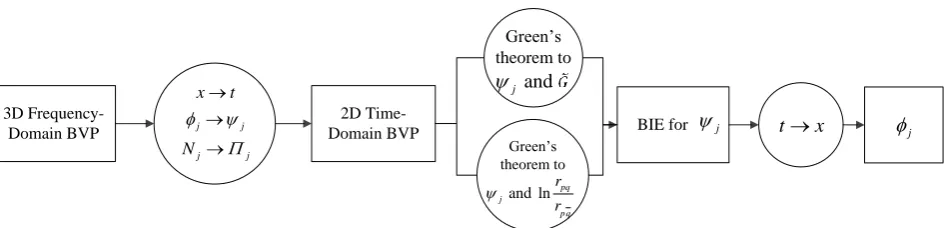
The flowchart for solving the mixed BVP using the 2.5D method is depicted in Fig.1. The BIE (16) or (17) derived from the mixed BVP are completely new. Comparing Eq.(16) with the BIE derived from the Neumann BVP (Ma et al., 2005), one can find that there is an additional term related to fluctuating air pressure in the
right-hand-most of Eq.(16), while the rest terms in two BIE are the same. One can even observe that the air pressure related term is a free surface memory term rather than an instantaneous one, which suggests that the
6
on the solution of the air cushion pressure.
3D
Frequency-Domain BVP j j
j j x t
N
2D Time-Domain BVP
Green’s theorem to
and
j
Green’s theorem to
and ln pq
j
p q
r r
[image:7.595.62.536.87.201.2]BIE for 12j tx j
Figure 1. The flowchart for solving the mixed BVP using the 2.5D method.
2.3. The computational complexity and numerical stability of the 2.5D method
As compared with the 3D methods, the major advantage of the 2.5D method is its higher computational efficiency. The analysis and comparison of computational complexity of the 2.5D method with the 3D methods can be roughly drawn out as follows.
Let 𝑀𝑠 be the number of sidehull or air cushion sections; 𝑁A and 𝑁B be the number of panels on each air
cushion and sidehull section, respectively; 𝑓(𝑘) and 𝐹(𝑘, 𝜃) be the integrand of the 2.5D method and the 3D Green’s function, respectively. Then similar to the computational complexity of the catamaran sidehulls (Duan et al., 2000; Guo et al., 2015), the computational complexity of the 2.5D method and the 3D methods for the SES can be written as, respectively
𝑃2.5D= 𝑂 (𝑀𝑠× (𝑁A+ 𝑁B)2× 𝑇(∫ 𝑓(𝑘)d𝑘 ∞
0 )) (20)
𝑃3D= 𝑂 (𝑀𝑠2× (𝑁A+ 𝑁B)2× 𝑇(∫ d𝜃 π
0 ∫ 𝐹(𝑘, 𝜃)d𝑘 ∞
0 )) (21)
where 𝑇(∙) represents the computational time for calculating the functions in the brackets. As 𝑀𝑠 is normally
much larger than one, the computational complexity of the 2.5D method is much less than the 3D methods. In numerical practice, generally the 2.5D method only takes a few minutes, while the 3D methods such as the 3D Rankine source method (Zhang et al., 2011) normally requires a few hours for solving the same problem.
It is worth noting that the matrix of the system equations generated by the abovementioned boundary element methods (BEM) is fully populated and unsymmetrical, which can significantly reduce the computational efficiency with the growth of panel number. Actually, the fast Fourier transform (FFT) methods (Zhang et al., 2011) or wavelet function methods (Karimi et al., 2005b; Karimi, 2006) can be employed to further enhance the efficiency of BEM. The investigation on this topic is beyond the scope of this paper, and will be carried out in our future works.
7
for evaluating the integral of the free-surface memory term with respect to time instead of the explicit method. More recently, Guo et al. (2018a; 2018b) incorporated the viscous dissipation effects into the free-surface equation and then developed a novel 2D time domain Green’s function, which was proved to have better numerical stability in evaluating the interaction between waves and floating bodies with flare angles. Nonetheless, the SES to be studied in this paper is almost wall-sided and not subjected to the issue of numerical instability, so no special treatments are needed. If the 2.5D method would be used for floating bodies with flare angles, the developments in Guo et al. (2018a; 2018b) should be implemented.
3. Motion equations for the SES
To validate the solution of the mixed BVP solved using the 2.5D method, the motion equations for the SES are briefly introduced in this section, through which the motion response and the fluctuating air pressure can be solved after the hydrodynamic parameters are given by the 2.5D method. Without loss of generality, the 5-DOF motions (the surge is always neglected in the 2.5D methods) of a SES advancing in regular waves of arbitrary
directions are considered, though only the heave and pitch motion of a SES in head waves will be investigated in
the next section.
3.1. Air dynamic equations
It is assumed that the variation of the fluctuating air pressure in the cushion along the vertical direction is not
significant in the SES and so the air pressure can be approximated by
𝑝̂(𝑥, 𝑦) ≅1ℎ∫ 𝑝(𝑥, 𝑦, 𝑧)d𝑧0ℎ (22)
where ℎ is the height of the air cushion; 𝑝(𝑥, 𝑦, 𝑧) is the fluctuating air pressure in the cushion that satisfies the
Helmholtz equation
∇2𝑝 + 𝑘 a
2𝑝 = 0 (23)
where 𝑘a= 𝜔/𝑐, 𝑐 is the sound speed.
Substituting Eq.(23) into Eq.(22), one obtains
(𝜕2
𝜕𝑥2+
𝜕2
𝜕𝑦2+ 𝑘a
2) 𝑝̂(𝑥, 𝑦) = −1 ℎ
𝜕𝑝 𝜕𝑧|
𝑧 = ℎ
𝑧 = 0 (24)
Taking Eq.(2) into account and using the momentum equation, Eq.(24) comes to
∑6+𝑁𝑗=7P𝜂𝑗( 𝜕2 𝜕𝑥2+
𝜕2 𝜕𝑦2+ 𝑘a
2) 𝑛
𝑗(𝑥, 𝑦) = − i𝜔ρa
ρwgℎ𝑤 |
𝑧 = ℎ
𝑧 = 0 (25)
where ρa is the density of air cushion, 𝑤 the air flow velocity along the vertical direction in the cushion. Multiplying Eq.(25) by 𝑁𝑖(𝑥, 𝑦), 𝑖 = 7, … ,6 + 𝑁P, and integrating the resulting equation with respect to
𝑥, 𝑦 on the horizontal section of the air cushion leads to
𝜂𝑖(𝑘a2− 4π2(( 𝛼
𝑙) 2
+ (𝛽
𝑏) 2
)) ∬ 𝑛𝑆P 𝑖2(𝑥, 𝑦)d𝑥d𝑦 = 𝜔2ρa
ρwgℎ(∬ 𝑛𝑆D 𝑖(𝑥, 𝑦)(𝜂3− 𝑥𝜂5+ 𝑦𝜂4)d𝑥d𝑦 −
∬ 𝑛𝑆 𝑖(𝑥, 𝑦)𝜁(𝑥, 𝑦)
P d𝑥d𝑦 + ∑ 𝑛𝑖(𝑥𝑗, 𝑦𝑗)𝑞𝑗
out 𝑁out
𝑗=1 − ∑ 𝑛𝑖(𝑥𝑗, 𝑦𝑗)𝑞𝑗in 𝑁in
𝑗=1 )− − − − (26)
where 𝑁out and 𝑁in are the number of air leakage holes and/or gaps and the number of air charge inflow holes,
respectively; 𝑞𝑗outand 𝑞𝑗in are the air leakage and inflow rate through 𝑗-th hole (gap), respectively; (𝑥𝑗, 𝑦𝑗) the
8 {
𝜁(𝑥, 𝑦) = 𝜁I(𝑥, 𝑦) + 𝜁D(𝑥, 𝑦) + 𝜁R(𝑥, 𝑦) + 𝜁P(𝑥, 𝑦) = 𝜁I(𝑥, 𝑦) + ∑6+𝑁𝑗=0P𝜂𝑗𝜁𝑗(𝑥, 𝑦)
𝜁I(𝑥, 𝑦) = 𝜂0e−i𝑘0(𝑥 cos 𝜃+𝑦 sin 𝜃)
𝜁D(𝑥, 𝑦) = 𝜂0𝜁0(𝑥, 𝑦) = − 𝜂0
g (i𝜔 − 𝑈 𝜕
𝜕𝑥) 𝜙0(𝑥, 𝑦, 0)
𝜁R(𝑥, 𝑦) = ∑6𝑗=2𝜂𝑗𝜁𝑗(𝑥, 𝑦)= − 𝟏
g∑ 𝜂𝑗(i𝜔 − 𝑈 𝜕
𝜕𝑥) 𝜙𝑗(𝑥, 𝑦, 0) 6
𝑗=2
𝜁P(𝑥, 𝑦) = ∑𝑗=76+𝑁P𝜂𝑗𝜁𝑗(𝑥, 𝑦)= ∑ 𝜂𝑗(𝑛𝑗(𝑥, 𝑦) − 1
g(i𝜔 − 𝑈 𝜕
𝜕𝑥) 𝜙𝑗(𝑥, 𝑦, 0)) 6+𝑁P
𝑗=7
(27)
where 𝜃 is the incident wave angle, and 𝑘0 the wave number. The first term on the right hand side of Eq.(27)
is the incident wave, while the rest terms are the disturbed waves due to unsteady motions and the fluctuating air
pressure of the SES.
There are 𝑁P air dynamic equations in Eq.(26), in which only motion or pressure amplitudes 𝜂𝑗, 𝑗 =
2, … ,6 + 𝑁P remain unknown. Eq.(26) actually builds up connections between motion responses and the
fluctuating air pressure.
3.2. Motion equations for the SES
The 5-DOF motion equations for the SES can be formulated as
∑ (−𝜔2(𝑀
𝑖𝑗+ 𝐴𝑖𝑗) + i𝜔𝐵𝑖𝑗+ 𝐶𝑖𝑗)𝜂𝑗 6+𝑁P
𝑗=2 = 𝐹𝑖, 𝑖 = 2, … ,6 (28)
where 𝑀𝑖𝑗, 𝐴𝑖𝑗, 𝐵𝑖𝑗, 𝐶𝑖𝑗 are the massor inertial moment of the SES, added mass, damping, restoring force matrix,
respectively, and 𝑀𝑖𝑗 = 0, 𝐶𝑖𝑗 = 0 for 𝑗 > 6; 𝐹𝑖 the wave fore along the 𝑖-th direction. As done in well-known
linear potential formulation, 𝐴𝑖𝑗 and 𝐵𝑖𝑗 are obtained through following equations
{𝐴𝑖𝑗 = Re{𝛬𝑖𝑗} 𝜔
2
⁄ 𝐵𝑖𝑗= − Im{𝛬𝑖𝑗} 𝜔⁄
(29)
𝛬𝑖𝑗 = −i𝜔ρw∬ 𝜙𝑆 𝑗𝑛𝑖d𝑠
B +ρw𝑈 ∬ 𝜙𝑆B 𝑗𝑚𝑖d𝑠−ρw𝑈 ∫ 𝜙𝐶𝐴 𝑗𝑛𝑖d𝑙 (30)
where 𝐶𝐴 is the stern section of the SES. The wave force 𝐹𝑖 could be decomposed into
𝐹𝑖 = 𝐹𝑖I+ 𝐹𝑖D+ 𝐹𝑖P (31)
where 𝐹𝑖I, 𝐹𝑖Dand 𝐹𝑖P are the F-K force, diffraction force and air dynamic force on the wet deck, respectively.
Their expressions are given as following
{
𝐹𝑖I= −𝜂0∙ i𝜌w𝜔0∬ 𝜙𝑆B 0𝑛𝑖d𝑠
𝐹𝑖D= 𝜂0∙ 𝛬𝑖0
𝐹𝑖P= −ρwg ∑ 𝜂𝑗∬ 𝑛𝑆D 𝑗(𝑥, 𝑦)𝑛𝑖(𝑥, 𝑦)d𝑥d𝑦 6+𝑁P
𝑗=7
(32)
Eq.(26) and Eq.(28) together with Eqs. (29)- (32) make up the closed equations for the SES, through which one can solve all motions and pressure amplitudes 𝜂𝑗, 𝑗 = 2, … ,6 + 𝑁P.
4. Application of the 2.5D method for solving the BVPs of the PACSCAT
In this section the solution of the mixed BVP obtained using the 2.5D method is validated through two cases, which evaluates the radiation wave on the interface due to fluctuating air pressure and solves heave and pitch
response as well as air dynamics of a PACSCAT running in regular head waves. Since the PACSCAT runs in
9
orthogonal Fourier modes from Eq.(3): 𝑁7(𝑥, 𝑦) = 1 and 𝑁8(𝑥, 𝑦) = sin(π𝑥 𝑙⁄ ) (𝑥m≅ 0 for the PACSCAT)
[image:10.595.55.533.163.305.2]are used in the following studies. Table 1 shows the principal parameters of the PACSCAT model. More detailed information and the body plan for the PACSCAT can be found in Guo et al. (2015).
Table 1. Principal parameters of the PACSCAT model (Guo et al., 2015).
Parameters Value Parameters Value
Mass (𝑀) 145 kg Moment of inertia for pitch (𝑀55) 77.4 kg·m2
Overall length (𝐿) 3.0 m
Static cushion overpressure (𝑝0)
760 Pa (𝐹𝑟𝑙 = 0.73)
Beam (𝐵) 0.7 m 510 Pa (𝐹𝑟𝑙 = 1.0)
Cushion length (𝑙) 2.5 m Air inflow rate (𝑄0) 150 m3/h
Cushion breadth (𝑏) 0.24 m Fan characteristic value (𝜕𝑄in⁄𝜕𝑝) -7.2E-5 m3/(s · Pa)
4.1. Radiation wave on the interface due to fluctuating air pressure
As shown in Eqs.(26)~(27), the radiation wave 𝜁P on the interface due to fluctuating air pressure on the
interface of the SES could have an impact on the motion responses, which suggests the importance of accurately predicting it. In many publications, however, the radiation wave 𝜁P was neglected (Faltinsen, 2005), or
approximated by solving the Dirichlet BVP (Doctors, 1976; Xie et al., 2008; Guo et al., 2017). Here we would like to compare the radiation wave 𝜁P of the PACSCAT by solving the Dirichlet BVP with the one by solving
the mixed BVP. Both of the mixed BVP and the Dirichlet BVP are solved using the 2.5D method.
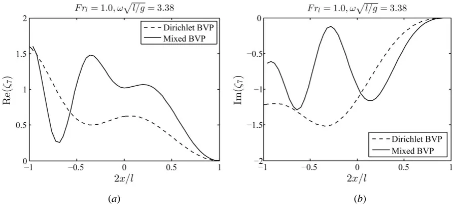
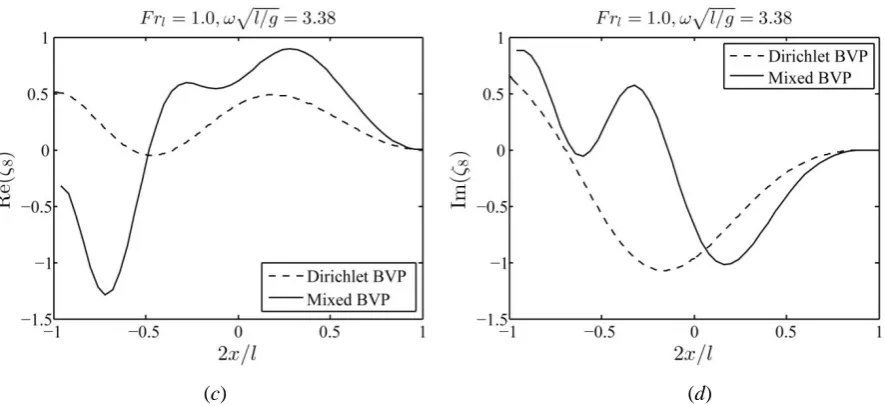
Fig.2 depicts the radiation wave profiles at the central longitudinal section 𝑦 = 0 for the cases of 𝐹𝑟𝑙= 1.0
and 𝜔√𝑙/𝑔 = 3.38. In the figure, (a) and (b) show the real and imaginary part of 𝜁7 while (c) and (d) give the
real and imaginary part of 𝜁8. In addition, the label ‘Dirichlet BVP’ and ‘Mixed BVP’ indicate that the
radiation waves are obtained by solving the Dirichlet and mixed BVP, respectively.
[image:10.595.70.519.528.744.2]10
[image:11.595.75.518.70.273.2](c) (d)
Figure 2. The profiles of radiation waves 𝜁7and 𝜁8 (defined in Eq.(27)) due to fluctuating air pressure at 𝑦 = 0
for 𝐹𝑟𝑙= 1.0 and 𝜔√𝑙/𝑔 = 3.38. ‘Dirichlet BVP’ and ‘Mixed BVP’ indicate the radiation waves obtained by
solving the Dirichlet and mixed BVP, respectively. (a) Real part of 𝜁7; (b) Imaginary part of 𝜁7; (c) Real part of
𝜁8; (d) Imaginary part of 𝜁8.
From Fig.2, one can find that the radiation wave from solving the Dirichlet BVP is very different from solving the mixed BVP, or more specifically, the latter is steeper than the former. This means that the coupling
between the fluctuating air pressure and sidehulls has significant influence on the radiation wave on the interface,
and the selective omission of the coupling effects could bring inevitable errors to the hydrodynamics of the air
cushion. The numerical results in this case also confirm the importance and necessity on solving the complete
mixed BVP to accurately predict the hydrodynamics of a SES.
4.2. Motion responses of the PACSCAT
The significant influence of coupling between the fluctuating air pressure and sidehulls on the radiation
wave profiles on the interface was demonstrated in Fig.2. It might be more interesting to investigate how the coupling effects make the difference in the seakeeping performance and air dynamics of the PACSCAT.
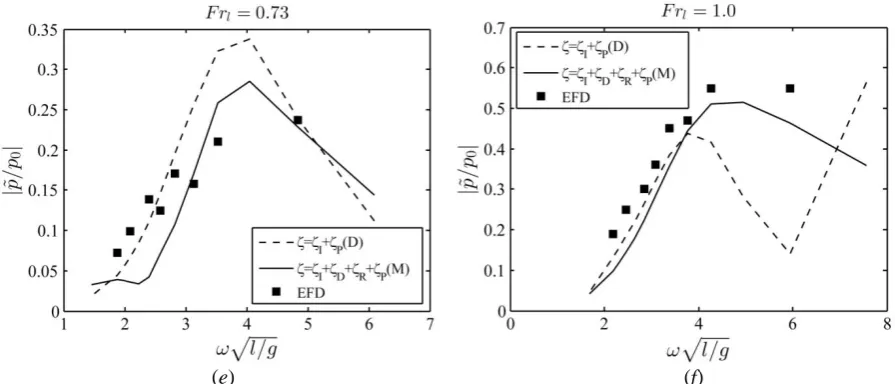
Fig.3 compares numerical results on the heave, pitch and fluctuating air pressure responses of the PACSCAT with the experimental data marked as ‘EFD’ under Froude number 𝐹𝑟𝑙 = 0.73 and 1.0. The results
labeled by ‘𝜁 = 𝜁I+ 𝜁P(D)’ are obtained from the potential model that considers the incident wave and the
radiation wave due to fluctuating air pressure on the interface by solving the Dirichlet BVP, while the sidehull
involved waves are not taken into account. The results labeled by ‘𝜁 = 𝜁I+ 𝜁D+ 𝜁R+ 𝜁P(M)’ are obtained
from the potential model that considers all possible waves on the interface, including the incident wave, diffraction and radiation wave of sidehulls, the radiation wave due to fluctuating air pressure by solving the
11
Yang et al. (2015), in which the bow fingers and stern seal bags of the PACSCAT are modeled as rigid bodies. Note that only the heave and pitch motion of the PACSCAT were presented in Yang et al. (2015), while the fluctuating air pressure was not given.
From Fig.3 (a)~(b) one can observe that two potential models generate the almost same heave RAOs in
large encountered frequencies (𝜔√𝑙/𝑔 > 4), but the results from model ‘𝜁 = 𝜁I+ 𝜁D+ 𝜁R+ 𝜁P(M)’ have
slightly better agreement with EFD data in the vicinity of natural frequency of the PACSCAT. Almost the same trend is obtained for the pitch RAO as shown in Fig.3 (c)~(d). The RANS solver underestimate the heave RAO under low encountered frequencies but overestimate it under high encountered frequencies. On the other hand, the RANS solver desirably predicts the pitch RAO under low encountered frequencies but significantly overestimates it under high encountered frequencies. From Fig.3 (e)~(f), it is more evident that the model ‘𝜁 = 𝜁I+ 𝜁D+ 𝜁R+ 𝜁P(M)’ significantly improves the numerical results of the fluctuating air pressure in the vicinity
of the resonance frequency. In contrast, the model ‘𝜁 = 𝜁I+ 𝜁P(D)’ overestimates the resonance peak of the
fluctuating air pressure at 𝐹𝑟𝑙 = 0.73, while underestimates that at 𝐹𝑟𝑙= 1.0.
(a) (b)
12
[image:13.595.71.519.72.264.2](e) (f)
Figure 3. A comparison of numerical results with experimental data marked as ‘EFD’ on seakeeping performance of the PACSCAT under Froude number 𝐹𝑟𝑙= 0.73 and 1.0. ‘𝜁 = 𝜁I+ 𝜁P(D)’ represents the numerical results
obtained from the model that considers the incident wave and the radiation wave due to fluctuating air pressure on
the interface by solving the Dirichlet BVP, while the sidehull induced waves are not taken into account. ‘𝜁 =
𝜁I+ 𝜁D+ 𝜁R+ 𝜁P(M)’ are obtained from the model that considers all possible waves on the interface, including
the incident wave, diffraction and radiation wave of sidehulls, the radiation wave due to fluctuating air pressure
by solving the mixed BVP. ‘CFD’ are the CFD results from Yang et al. (2015). (a~b) Heave RAO; (c~d) Pitch RAO; (e~f) Fluctuating air pressure RAO.
The numerical results suggest that the coupling effects could have significant influence on the air cushion
dynamics, and the 2.5D method is helpful to capture the effects as well as to improve the numerical results on motion response and the fluctuating air pressure.
5. Conclusions
This paper firstly presents the 2.5D method to solve the mixed BVP of a SES consisting of homogeneous Neumann boundary condition on the sidehulls and nonhomogeneous Dirichlet boundary condition on the
interface. This kind of problem has never been dealt with by the 2.5D method before. The newly developed 2.5D method allows one to consider the coupling between the fluctuating air pressure and sidehulls, which is usually ignored in other publications.
The solution of the mixed BVP obtained using the 2.5D method is validated by applying it on a special SES – PACSCAT through two cases. The first case is to evaluate the radiation wave due to fluctuating air pressure
on the interface. The numerical results confirm that the radiation wave from solving the Dirichlet BVP (Doctors,
1976; Xie et al., 2008; Guo et al., 2017) is very different from solving the complete mixed BVP, i.e. the sidehull
effects have significant impact on the radiation wave and should not be ignored. The second case is employing
the 2.5D method to calculate the relative hydrodynamic parameters of the PACSCAT and solve the motion equations to obtain the seakeeping performance of the PACSCAT. The numerical results suggest that the 2.5D method is able to capture the sidehull effects and to improve the predicted results of the fluctuating air pressure.
13 more numerical tests are expected to be carried out in the future.
Acknowledgments: This project is supported by the National Natural Science Foundation of China (Grant
no.51509053, no.51579056 and no.51739001). The second author wishes to thank the Chang Jiang Visiting Chair professorship of Chinese Ministry of Education, supported and hosted by the HEU.
References
Bhushan, S., Mousaviraad, M., Stern F., 2017. Assessment of URANS surface effect ship models for calm water
and head waves. Applied Ocean Research, 67: 248-262.
Connell, S.B., Milewski, M.W., Goldman, B., Kring, C.D., 2011. Single and multi-body surface effect ship
simulation for T-Craft design evaluation. Proceedings of the 11th International Conference on Fast Sea
Transportation. FAST 2011. Honolulu, Hawaii, USA, pp.130–137.
Dai, Y.S., Duan, W.Y., 2008. Potential Flow Theory of Ship Motions in Waves. 1st ed., The National Defense Industries Press: Beijing, China, pp. 248–249.
Doctors, L.J., 1976. The effect of air compressibility on the nonlinear motion of an air-cushion vehicle over waves.
Proceedings of the 11th ONR Symposium on Naval Hydrodynamics. UCL, London, UK, pp.373–388.
Duan, W.Y., 1995. Nonlinear Hydrodynamic Forces Acting on a Ship Undergoing Large Amplitude Motions. Ph.D. Thesis, Harbin Engineering University, Harbin, China.
Faltinsen, O., Zhao, R., 1991. Numerical predictions of ship motions at high forward speed. Philos. Trans. R. Soc.
Lond, A, 334: 241-252.
Faltinsen, O.M., 2005. Hydrodynamics of high-speed marine vehicles, 1st ed., Publisher: Cambridge University
Press, UK, p.141- 163.
García-Espinosa, J., Capua, D.D., Serván-Camas, B., et al., 2015. A FEM fluid–structure interaction algorithm
for analysis of the seal dynamics of a Surface-Effect Ship. Computer Methods in Applied Mechanics &
Engineering, 295: 290-304.
Guo, Z.Q., Ma, Q.W., Yang, J.L., 2015. A seakeeping analysis method for a high-speed partial air cushion
supported catamaran (PACSCAT). Ocean Eng., 110: 357-376.
Guo, Z.Q., Ma, Q.W., Sun, H.B., Hao, H.B., 2017. 2.5D method for pulsating pressure induced waves on the free
surface. Proc. of 27th International Ocean and Polar Engineering Conference (ISOPE 2017), San Francisco,
California, USA, June 25-30, p.1029-1033.
Guo, Z.Q., Ma, Q.W., Qin, H.D., 2018a. A time-domain Green’s function for interaction between water waves and floating bodies with viscous dissipation effects. Water, 10, 72.
Guo, Z.Q., Ma, Q.W., Yu, S.R., Qin, H.D., 2018b. A body-nonlinear Green’s function method with viscous dissipation effects for large-amplitude roll of floating bodies. Applied Sciences, 8(4), 517.
Karimi, H.R., Maralani, P.J., Lohmann, B., et al., 2005a. H∞ control of parameter-dependent state-delayed
systems using polynomial parameter-dependent quadratic functions. International Journal of Control, 78(4): 254-263.
14
Karimi, H.R., 2006. Optimal vibration control of vehicle engine-body system using haar functions. International Journal of Control Automation & Systems,4(6): 714-724.
Karimi, H.R., Duffie, N.A., Dashkovskiy, S., 2010. Local capacity $h_{\infty}$ control for production networks of autonomous work systems with time-varying delays. Automation Science & Engineering IEEE Transactions on, 7(4): 849-857.
Lee, C.H., Newman, J.N., 2015. An extended boundary integral equation for structures with oscillatory
free-surface pressure. International Journal of Offshore & Polar Engineering, 1: 347-353.
Ma, S., Duan, W.Y., Song, J.Z., 2005. An efficient numerical method for solving ‘2.5D’ ship seakeeping problem.
Ocean Eng, 32(8–9): 937–960.
Xie, N., Vassalos, D., Jasionowski, A., Sayer, P., 2008. A seakeeping analysis method for an air-lifted vessel.
Ocean Eng, 35: 1512-1520.
Yang, J.L., Sun, H.B., Guo, Z.Q., 2015. Study on motion of partial air cushion support catamaran in regular waves. J. Huazhong Univ. Sci. & Tech. (Natural Science Edition), 43(11): 104-109.
Zhang, S., Weems, K., Lin, W.M., 2011. Solving nonlinear wave-body interaction problems with the pre-corrected fast fourier transform (pFFT) method. In: Proceedings of the 11th International Conference on Fast Sea Transportation. FAST 2011. Honolulu, Hawaii, USA, pp. 153-160.