Anatomically Realistic Structural Modeling of the Cardiac Purkinje Network: A Basis for Studying Contributions of the Conduction System to Ventricular Arrhythmias

(1)

Rochester Institute of Technology

RIT Scholar Works

Theses

Thesis/Dissertation Collections

5-9-2014

Anatomically Realistic Structural Modeling of the

Cardiac Purkinje Network: A Basis for Studying

Contributions of the Conduction System to

Ventricular Arrhythmias

Benjamin Liu

Follow this and additional works at:

http://scholarworks.rit.edu/theses

This Thesis is brought to you for free and open access by the Thesis/Dissertation Collections at RIT Scholar Works. It has been accepted for inclusion in Theses by an authorized administrator of RIT Scholar Works. For more information, please contactritscholarworks@rit.edu.

Recommended Citation

(2)

Anatomically Realistic

Structural Modeling

of the Cardiac Purkinje Network

A Basis for Studying Contributions

of the Conduction System to Ventricular Arrhythmias

by

Benjamin Liu

A Thesis Submitted in Partial Fulfillment of the Requirements

for the Degree of Master of Science in Applied and Computational Mathematics

School of Mathematical Sciences, College of Science

Rochester Institute of Technology

Rochester, NY

(3)

Committee Approval:

Dr. Elizabeth Cherry

School of Mathematical Sciences

Thesis Advisor

Date

Dr. Matthew Hoffman

Committee Member

Date

Dr. David Ross

Committee Member

Date

Dr. Nathan Cahill

Director of Graduate Programs

(4)

Abstract

A cardiac arrhythmia is a potentially-lethal event in which the normally orderly electrical

activity in the heart is disrupted – it becomes disorganized and compromises effective

contrac-tion. To better understand arrhythmia dynamics to develop potential therapies and treatments,

experimental, computational, and mathematical tools are required. Simulations of cardiac tissue

provide valuable insight into the dynamics of life-threatening cardiac arrhythmias, and though

much work has been done in this area, the role of the Purkinje network during ventricular

ar-rhythmias has largely been ignored. The function of the Purkinje network is crucial to normal

heart rhythm, so its inclusion into cardiac structural models is a necessary step to furthering our

understanding of arrhythmias. Current technological limitations prevent the direct imaging of

the intact three-dimensional Purkinje structure, making the incorporation of a Purkinje network

into such simulations difficult. At this time most efforts involve generating artificial Purkinje

networks either through manual drawing of Purkinje-like structures or through algorithms that

generate the structures procedurally based on rules gleaned from physiological studies. Very

lit-tle work has focused on the incorporation of a Purkinje network based directly on experimental

data. Through dissection, photographs of the Purkinje network can be taken, but these

two-dimensional photographs do not capture the three-two-dimensional structure of the network. Here

we present a novel method for reconstructing the three-dimensional Purkinje structure based

on projecting two-dimensional Purkinje structures recovered from experimental photographs

onto realistic ventricular geometries. The resulting three-dimensional Purkinje structures make

possible the modeling of the coupled ventricle-Purkinje system. The second major component

of our work is the development of two methods by which these systems can be modeled. We

implement these models using real anatomical data and find good agreement between the two

models and with previous experimental studies. Our work provides a basis for the further study

of ventricular arrhythmias, and in particular the role the Purkinje network plays in initiating

(5)

Acknowledgements

(6)

List of Figures

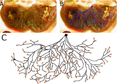
1 Activation sequence of the human heart. Plots show isochronal maps of the acti-vation time of the tissue at each point. The heart is shown in a split view with the main segment in an anterior orientation. Activation begins primarily from the left endocardial surface, and the right ventricular free wall is the last region to be activated. Modified from Ref. [11]. . . 10 2 Digitization of the canine left ventricular Purkinje network. (A) Photograph from

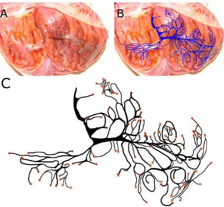
experiment in which the left ventricle was dissected and treated with Lugol’s solution, staining the Purkinje network darker than surrounding tissue. The Purkinje network is visible to the eye. The left bundle branch is visible in the center at the top of the photograph, which corresponds to the septum wall. (B) Visible Purkinje fibers are manually traced in an image-editing program; the resulting network structure is overlaid for comparison onto the photograph from which it was extracted. (C) The resulting digitized Purkinje structure. Coupling sites – located at the ends of the fibers – are indicated by orange circles. . . 15 3 Digitization of the canine right ventricular Purkinje network. (A) Experimental

(9)

4 Isosurfaces of the canine ventricular structure used in our work. (Left) The en-tire ventricular structure in a posterior viewing orientation. (Center) Transparent overlay of the epicardial surface in line with the endocardial surfaces, shown for comparison and orientation. The left endocardial surface is shown in orange and the right endocardial surface is shown in blue. (Right) Alternate viewing angle of the isolated endocardial surfaces of the left and right ventricles. . . 17 5 Isosurfaces of the rabbit ventricular structure used in our work. (Left) The

en-tire ventricular structure in a posterior viewing orientation. (Center) Transparent overlay of the epicardial surface in line with the endocardial surfaces, shown for comparison and orientation. The left endocardial surface is shown in orange and the right endocardial surface is shown in blue. (Right) Alternate viewing angle of the isolated endocardial surfaces of the left and right ventricles. . . 18 6 A choice of a curve C and the associated cylinder with base C. (Left) The curve

in the plane is shown in red; the associated cylinder is shown in a different viewing angle. (Center and Right) The cylinder chosen to approximate an endocardial surface is shown aligned with the surface. . . 21 7 The vector fieldV~ and its solution trajectories. (Left) Shown in red is the

outward-pointing unit normal vectorN~(s) to the curveC, shown in black. The blue vectors show a sampling of the vector fieldV~, defined everywhere. (Right) The curvilinear coordinate system resulting from taking solution trajectories to the vector field V~. Shown in blue is the original curveC; solid black lines (and the orange dashed curve) are solution trajectories representing lines of constant s in the coordinate system, and black dashed lines are lines of constant t. Note that where solution trajectories intersectC, they are orthogonal toC. . . 22 8 Schematic diagram of a Bezier Curve. The third-degree Bezier curve (black) is

(10)

9 (Top) The vector field V for various values ofP and (Bottom) associated induced curvilinear coordinate systems. Lower values of P result in ‘smoother’ trajectories that quickly deviate from the direction normal to the curve, whereas larger parameter values result in ‘sharper’ trajectories that follow more closely the direction normal to the curve. . . 27 10 Visualizations of the canine left ventricular endocardial surface and the curve and

associated cylinder chosen to approximate the surface. (Left) Plots show the cho-sen curveC and the resulting curvilinear coordinate system plotted against various contour lines from cross-sections of the endocardial surface. The chosen curve fairly well approximates the surface and its contour lines with agreement being best in the middle contours, or between the base and apex of the ventricle. The curve and contours coincide particularly well near the septum wall. (Right) Plot shows an iso-surface of the endocardial iso-surface (grey), the approximating cylinder (transparent) and the same contour lines used in the left plots superimposed onto the surface for reference. The view is facing the septum wall. . . 29 11 Visualizations of the texture mapping of the canine left Purkinje network onto the

ca-nine left ventricular endocardial surface. The extent of the texture-mapped network is nearly that of the entire endocardial surface. . . 30 12 Visualizations of the canine right ventricular endocardial surface and the curve and

(11)

13 Visualizations of the texture mapping of the canine right Purkinje network onto the canine right ventricular endocardial surface. The extent of the network is limited. This coincides with experimental observations near the septum wall, but network coverage of the free wall is observed to be greater than achieved here, particularly near the apex. . . 32 14 Visualizations of the rabbit left ventricular endocardial surface and the curve and

associated cylinder chosen to approximate the surface. (Left) Plots show the chosen curveC and the resulting curvilinear coordinate system plotted against various con-tour lines from cross-sections of the endocardial surface. The curve coincides with the surface particularly closely near the septum wall and at the base of the ventricle. The approximation worsens nearer the apex. (Right) Plot shows an isosurface of the endocardial surface (grey), the approximating cylinder (transparent) and the same contour lines used in the left plots superimposed onto the surface for reference. The view is facing the septum wall. . . 33 15 Visualizations of the texture mapping of the canine left Purkinje network onto the

rabbit left ventricular endocardial surface. The extent of the texture mapped network is nearly that of the entire endocardial surface. . . 34 16 Visualizations of the rabbit right ventricular endocardial surface and the curve and

associated cylinder chosen to approximate the surface. (Left) Plots show the chosen curveC and the resulting curvilinear coordinate system plotted against various con-tour lines from cross-sections of the endocardial surface. The curve coincides with the surface particularly closely near the septum wall and between the ventricle base and apex. The approximation worsens near both the apex and the base. (Right) Plot shows an isosurface of the endocardial surface (grey), the approximating cylin-der (transparent) and the same contour lines used in the left plots superimposed onto the surface for reference. The view is facing the septum wall. . . 35 17 Visualizations of the texture mapping of a Purkinje network onto the rabbit right

(12)

18 Results from Cherry and Fenton’s coupled ventricle-Purkinje model, shown here to illustrate the coupling between the constituent ventricle and Purkinje models. Plots show ventricular tissue and Purkinje network 7 ms after the Purkinje network was activated; about half of the network coupling sites have been activated, and tissue is being activated by the network. Orange dashed lines show some of the many (130) ventricle-Purkinje coupling sites. Green lines at the sides of the ventricle plot indicate periodic boundary conditions; all other boundary conditions are no-flux. . . 39 19 Schematic visualization of a 3D-3D model. The structure is a simplified contrived

structure used for illustrative and test purposes only and is not anatomically real-istic. (Left) View of the test geometry. (Right) View of the conduction system test geometries. Dashed lines show some of the many couplings between Purkinje networks and the ventricles. . . 41 20 Schematic visualization of a 3D-2D model. The structure is a simplified contrived

structure used for illustrative and test purposes only, and is not anatomically real-istic. (Left) View of the test geometry. (Right) View of the conduction system test geometries. Dashed lines show some of the many couplings between Purkinje networks and the ventricles. . . 43 21 Comparison of phase fields resulting from the original and modified relaxation

al-gorithm. The original mask has a grid spacing of ∆x = .1, and both phase-field generation methods are run with the interface width ξ = .2. (Left) The Boolean input mask defining a thin annular domain. (Center) The phase field resulting from the application of the original relaxation algorithm to the input mask. Note that the top, bottom, left, and right parts of the annulus have low φ values, which compro-mises the connectivity of the domain. (Right) The phase field resulting from the application of the modified relaxation procedure with the added boundary condition. The entire original annular region has a value ofφ= 1, ensuring connectivity. . . 44 22 Test structure used in the test problem. (Left) The entire test structure – a

(13)

23 Diagrams showing the conduction systems used in the test problem. These simple contrived networks serve to validate model coupling and are not meant to model the genuine Purkinje network structure. Red represents the network, yellow the coupling sites, and magenta the stimulus sites. (Left) Left Purkinje network. (Right) Right Purkinje network. . . 48 24 Activation times of the main structure in the test 3D-3D model. Plots show isochronal

maps of activation times in a split view. . . 50 25 Activation times of the main structure in the test 3D-2D model. Plots show isochronal

maps of activation times in a split view. . . 50 26 Comparison of activation times in the 3D-3D and 3D-2D model implementations of

the test problem. Plots show at each point in the tissue the activation time of the 3D-3D model minus the activation time of the 3D-2D model. Colors are given so that white areas indicate near agreement of the two models, green indicates a positive difference (3D-2D has earlier activation), and red a negative difference (3D-3D has earlier activation). . . 51 27 Isochronal plots showing activation times of the rabbit ventricles in the 3D-3D model. 52 28 Isochronal plots showing activation times of the rabbit ventricles in the 3D-2D model. 53 29 Comparison of activation times in the rabbit ventricles in the 3D-3D and 3D-2D

(14)

1 Introduction

Heart disease is a term for a broad class of afflictions of the cardiovascular system; as a leading cause of death worldwide, efforts in many different fields are being made to combat it. While certain types of heart disease are genetic, progressive, or otherwise diagnosable, others, like cardiac arrhythmias, can occur suddenly and without warning, making them very dangerous and difficult to prevent. Cardiac arrhythmias are disruptions in the normal electrical activity of the heart. The heart functions through mechanical contraction, which is a byproduct of electrical excitation of the cardiac tissue. Disruptions in this electrical activity can therefore compromise the contraction of the cardiac muscle, leading to ineffective pumping of blood. While some types of arrhythmias have little noticeable effect, others are potentially lethal and can lead to sudden cardiac death.

Ventricular arrhythmias are especially dangerous because of the critical role the ventricles play in normal heart rhythm. The ventricles are thick, muscular chambers that actively pump blood out of the heart and throughout the body. Ventricular arrhythmias can rapidly become life-threatening if normal electrical activity is not restored, which usually requires the use of aggressive techniques such as defibrillation.

To facilitate the timely and correct sequence of activation of the ventricles, a specialized electrical conduction system called the Purkinje network exists within the ventricles. The Purkinje network functions to distribute stimuli throughout the entire ventricles, leading to a much faster total activation of the ventricles than could be achieved by the spread of excitation solely through the ventricular muscle tissue. The role of the Purkinje network is crucial during normal heart rhythm, but much less is known regarding its function during ventricular arrhythmias. Some experiments have shown that the Purkinje network may be important to the genesis of certain types of arrhythmias [18] and that the absence of the network can alter arrhythmia dynamics [10], but further study is needed to improve our understanding of the effect of the Purkinje network during such events.

(15)

phenomena. Simulation yields easily reproducible results, a great boon particularly in a biological field. The study of arrhythmias in the form of re-entrant electrical waves benefits greatly from the use of modeling and simulation because such results can provide insights otherwise unattainable solely through experimentation [1, 27, 2, 21, 9, 32, 17, 19]. Experimentally, many features of interest cannot be observed such as wave behavior within the interior of the muscle, but in simulation every aspect of the model is available for inspection and review.

While modeling efforts have produced many valuable insights regarding cardiac arrhythmias in gen-eral, comparably fewer studies have investigated the role of the Purkinje network during ventricular arrhythmias. Such studies require the incorporation of a structural model of the Purkinje network, and at present physical and experimental limitations make the retrieval of the physical Purkinje network structure impossible. Most studies that have modeled the Purkinje network structure have therefore constructed artificial Purkinje networks that are often either hand-drawn or in some cases generated algorithmically based on fractal-like branching structures. These artificial networks are often incorporated into ventricular models with the goal of reproducing normal activation times and sequences to match experimental observations.

A key feature of the development of current Purkinje structural models is that their construction is designed or guided by the modeler. One methodology that would avoid this shortcoming is to base Purkinje structural models directly on anatomical data; unfortunately, it is not currently possible to capture the intact three-dimensional Purkinje network structure. One recent study has attempted to overcome this limitation by making use of imaging data of the Purkinje network in the form of photographs. In 2012 Cherry and Fenton made use of the fact that the Purkinje network can be revealed through dissection of the ventricles to obtain two-dimensional photographs of the network structure [7]. In their work, they used these photographs to create two-dimensional Purkinje structural models and created a model of the combined ventricle-Purkinje system. Their work was the first instance of a Purkinje structural model based directly on anatomical data. The goal of this thesis is to extend this recent approach to accurately model and incorporate the three-dimensional Purkinje structure into an anatomically realistic model of the ventricles. The development of these models for the ventricular system will form a basis for the further study of ventricular arrhythmias and the effect the Purkinje network has on arrhythmia dynamics in the ventricles.

(16)

(17)

2 Overview of Cardiac Anatomy and Models

2.1 Cardiac Tissue as an Excitable Medium

In investigating cardiac arrhythmias, we study cardiac cells and tissue as an excitable medium. Excitable media are characterized by several important properties: a stable rest state, a stimulus threshold, excitability, refractoriness, wave propagation without damping, and the support of spiral and scroll waves [16].

A cardiac cell is an excitable medium. Its stable rest state is characterized by the cell membrane potential settling to a resting value of around -80 mV, along with there being no net transport of ions across the cell membrane. A cardiac cell has a stimulus threshold of around -60 mV [22]; stimuli that cause the membrane potential to rise above this level will cause the cell to excite. The form an excitation takes on in cardiac cells is that of the cardiac action potential (other types of cells can have slightly different characterizations): an abrupt depolarization of the cell membrane potential from its resting potential followed by a much more gradual repolarization back to the resting potential. Cardiac cells are refractory in that after generating an action potential, they cannot generate any further responses to stimuli for some time; in essence, the cell must recover after generating a response.

Cardiac tissue is composed of many cardiac cells coupled electrically in a diffusive manner. Physi-ologically, the mechanism behind the coupling of cells is gap junctions – specialized structures that connect cells [28]. Through this coupling, action potentials generated in a cell can induce action po-tentials in neighbor cells. This coupling results in the support of waves of depolarization that spread throughout tissue; exciting a small patch of cardiac tissue will result in an outward-propagating wavefront that does not damp out over time.

(18)

complex phenomena involving re-entrant waves do not subside naturally. In patients, such electrical behavior in the heart results in various cardiac arrhythmias. A single re-entrant wave is often the cause of tachycardia, a type of arrhythmia in which many rapid heartbeats are registered. This can often transition into the more serious condition of ventricular fibrillation, which is caused by the emergence of several re-entrant waves, typically after a single re-entrant wave ‘breaks’ into multiple waves. In these cases, the patient typically must be subjected to defibrillation, in which electrodes are used to force all tissue in the heart to depolarize or repolarize, thereby ‘resetting’ the tissue in order to disrupt the re-entrant waves.

2.2 Cardiac Cell Models

Cardiac cell dynamics are often modeled with systems of ordinary differential equations [12, 15]. Such models may either be phenomenological or function by modeling intracellular dynamics. These latter models are referred to as ionic models because they model the membrane potential by track-ing various transmembrane ion currents [12]. The equations of such systems are typically highly nonlinear and the number of variables in the systems varies greatly among models. There are popular two- and three-variable models [23, 20, 13] as well as much more complex and detailed models with dozens of variables [12, 15]. Smaller models are well-suited for studying tissue-level phenomena such as spiral- and scroll-wave dynamics, whereas more complex models are more often used in the study of cellular dynamics. Regardless of the level of detail or sophistication of these models, they most commonly can be expressed in the form

dV dt =−

Iion

Cm

, (1)

whereV is the membrane potential of the cell,Cmis the membrane capacitance of the cell, andIion

is the sum of various transmembrane currents, usually governed by several other time-dependent variables. Thus (1) actually is one of a system of equations that in some models can be highly complex. Other model equations can be summarized by

d~y

dt =f(~y, V, t),

where ~y is a vector referring to the various model variables. These model variables are typically ionic current gating variables or intracellular ion concentrations [12].

(19)

2.3 Modeling Cardiac Tissue

Cardiac tissue is often modeled as a continuum of cardiac cells [8]. In this manner, the cardiac cell equation (1) can be transformed into a reaction-diffusion equation, where an ionic model for cardiac cells governs the reaction and the membrane potential is allowed to diffuse spatially according to the Laplacian. In this way, an ODE model for cardiac cells can be turned into a PDE for cardiac tissue, as in (2).

∂V ∂t =−

Iion

Cm

+D∆V (2)

Here D is the diffusivity of the membrane potential. Typically, no-flux or periodic boundary conditions are also imposed when using such a model.

Tissue-level simulations can be as simple as solving the cardiac reaction-diffusion equations on one-dimensional cables or on rectangular domains. In these simulations, many phenomena of interest to the study of cardiac arrhythmias can appear, such as spatially concordant and discordant electrical alternans, spiral waves, and wave break.

The physical structure of the domain on which the cardiac reaction-diffusion equations are solved can have a significant affect on the various arrhythmic phenomena that the tissue can support. One canonical example is that of an annulus-shaped tissue; in such a domain, the tissue itself supports a type of re-entrant wave in which the wave front propagates around the ring continuously. Such anatomically-supported re-entrant waves are referred to as anatomical re-entrant, whereas a spiral wave revolving around a spiral tip is referred to as functionally re-entrant. While similar behavior can occur in rectangular domains in the form of a spiral wave, such a wave will have a spiral tip around which it revolves, whereas in the case of the annular domain, the central void functions as an anatomical feature that ‘pins’ the reentrant wave.

2.4 Whole-Heart and Ventricle Simulations

(20)

the direction parallel to the fibers and more slowly perpendicular to the fiber direction [28]. A typical ratio of the parallel and perpendicular diffusivities is 5 : 1 to 10 : 1 [14, 8]. The physical reason for this is the density of gap junctions is greater at the ends of the cells, relative to the fiber orientation. To account for this, the cardiac reaction-diffusion equations (2) can be modified [13] by the introduction of a local fiber orientation tensor D(x).

∂V ∂t =−

Iion

Cm

+∇ ·D(x)∇V (3) Whereas previously in (2) the parameter D was a scalar, here D(x) is a tensor defined over the domain of interest, that accounts for the increased conductivity in the direction of the fibers. The heart is composed of many layers of muscle that lie in varying orientations; the variety in fiber orientation makes the uniform contraction of the cardiac muscle possible. It is commonly regarded that these layers are parallel to the inner and outer surfaces of the heart, so the fiber direction of each layer lies primarily in this plane. Fibers typically follow approximate geodesic lines as they wind their way around the heart [26]. Moving from the endocardium to the epicardium, the fiber orientation within each layer changes [30, 24]. In reality, the distinction of there being discrete layers is made more for illustrative purposes; the layers in fact form a continuum, with the fiber orientation changing smoothly between some angleθi with respect to the axis normal to the cardiac

surface at the endocardium and some angle θf at the epicardium.

Whole-heart simulations provide useful information about how the anatomical structure of the heart can affect arrhythmia dynamics. Such simulations consist of solving the cardiac reaction-diffusion equations on anatomically-realistic domains, recovered experimentally from real hearts. Anatomical data sets can be obtained through several means, such as dissection [24, 29] or image segmentation of MRI scans of an intact heart [3]. The means by which such models are implemented computationally are most often finite differences or finite elements. Finite-element methods natu-rally support domains of arbitrary structure, most often specified by a triangulated mesh surface or volume. Implementations utilizing finite differences require additional tools to implement arbitrary domains, such as in the work by Fenton et al. in which the phase-field method was used [14], or variations such as that of Buzzard et al. [5]. In our work we utilize a finite-difference scheme, and a more in-depth discussion of the topic can be found in Section 5.

(21)

electrically insulated from one another, making the study of the ventricles in isolation a reasonable simplification.

2.5 Cardiac Anatomy and Normal Heart Rhythm

The heart is composed of four chambers: two atria and two ventricles. The atria act to receive blood and are significantly smaller than the ventricles, which fill with blood from the atria and then expel it from the heart through contraction. When the heart is functioning healthily and normally, it is undergoing normal heart rhythm. Normal heart rhythm consists of several events, the timing of which is important to produce an effective contraction to pump blood. We have so far in our discussion focused mainly on the electrophysiological properties of cardiac cells and tissue rather than mechanical or contractile properties. Though contraction of the heart can have some effect on the electrical activity of the heart, this effect is usually minimal. Conversely, the mechanical contraction of cardiac tissue is a response usually directly related to the electrical activity. The timing of electrical events is thus important to produce muscle contraction, and disorganized electrical activity amounts to disorganized contraction.

(22)

normal repolarization would facilitate.

2.6 The Purkinje Network

The Purkinje network has a vital role in normal heart rhythm. While the atria have a somewhat less complicated role than the ventricles of passively filling with blood, the ventricle serve to pump blood out of the heart and throughout the body through contraction. The Purkinje network is necessary to quickly initiate coordinated depolarization across each ventricle because of the large musculature of the ventricles, the relatively slow conduction velocity of normal cardiac tissue (about a fourth of the conduction velocity of Purkinje fibers), the activation sequence needed in the ventricles to produce an effective contraction, and the timescale on which excitation must occur.

(23)

[image:23.612.76.538.77.425.2]

(24)

3 Research Aim and Prior Work

3.1 Prior Work

As discussed in Section 1, the Purkinje network is crucial to normal heart rhythm. The effect of the Purkinje network during ventricular arrhythmias is much less well understood. Experimentally, evidence suggests that the Purkinje network may play a significant role in ventricular fibrillation. In 1995, Janse et al. compromised the Purkinje network in pig ventricles by cryoablating the endocardium and found that ventricular fibrillation could no longer be initiated [18]. In 2008, Dosdall et al. produced similar results after chemically ablating the Purkinje network in canine hearts: ventricular fibrillation terminated more quickly [10]. Many modeling efforts have been made to incorporate Purkinje-like networks into ventricular models. Though many methodologies have been employed in the creation of these networks, common to almost all modeling efforts so far is that the Purkinje network is manually or artificially generated rather than being based on anatomical data.

In several studies, relatively simple Purkinje networks have been constructed to mimic known anatomical features of the Purkinje network, such as its position and coverage of the endocardial surfaces. In 1998 Berenfield and Jalife created a Purkinje structural model by a procedure in which a manually drawn Purkinje network was projected onto the endocardial surface by “laying it onto the detected endocardial surfaces” [2]. The exact procedure by which this was accomplished was not detailed extensively, nor was it the focus of their work; rather, their goal was the creation of a structure having Purkinje-like characteristics, such as extent and area of the endocardial surfaces covered by the network. Clements and Vigmond developed a procedure by which a ventricular anatomical structure in the form of a triangulated mesh could be used to develop a Purkinje structural model [9, 32]. Their method began by first isolating the portion of the model mesh constituting the endocardial surfaces. A sophisticated flattening algorithm then was used to map the triangles in the endocardial meshes to the plane. Next, a manually drawn Purkinje network was laid onto the endocardial surfaces and the flattening transformation was inverted, yielding a three-dimensional Purkinje structure compatible with the initial cardiac structure.

(25)

Purk-inje network was generated to primarily activate regions of the ventricles observed experimentally to be sites of first activation [27]. Simelius et al. used a similar approach to design a model of the ventricular system that produced activations consistent with observed activation sequences and timings of the human heart, as well as with ECG data [21]. In 2008, Tusscher and Panfilov created a ventricular model incorporating a conduction system to investigate the role of the Purkinje net-work in normal and abnormal conduction [19]. Their approach to generating a Purkinje netnet-work relied on user-specified terminal Purkinje fiber sites, which were then used to generate the full network.

Some work has done in constructing Purkinje-like networks by generating branching structures based on fractal-like patterns. In 1991, Abboud et al. modeled the Purkinje network for use in reproducing ECG data through simulation [1]. In their work, the Purkinje network was modeled as a self-similar branching tree structure, in which the initial His bundle connection of the network divided symmetrically into two smaller branches, which each further divided into smaller branches. In 2008, Ijiri et al. developed an algorithm based on the L-system for generating Purkinje networks given a cardiac structure [17] and limited user input. The L-system is a formal grammar that can implement a system for generating fractal-like structures based on simple rules, originally developed for modeling plant cells and structures. In their work, Ijiri et al. used the L-system to generate a branching mesh structure that was confined to the endocardial surface starting from a number of user-defined ‘terminal locations’.

All of the methods for constructing Purkinje networks so far discussed have used either hand-drawn or computer-generated networks based on general principles. Very little work has been done on using experimental data to directly create Purkinje structures. The reason for this is most probably technological limitations: MRI and other means by which three-dimensional structures may be isolated cannot be applied to capture the Purkinje structure because there is little to no difference in Purkinje muscle density as compared to the surrounding cardiac tissue.

(26)

digitized Purkinje structure for use in a ventricle-Purkinje simulation [7].

Cherry and Fenton’s ventricle-Purkinje model was the first structural model of the Purkinje network based directly on experimental data. Their work showed that the integration of a Purkinje network into simulations of cardiac tissue can lead to significant differences in arrhythmia dynamics. Their work integrated a Purkinje network into a cylindrical cardiac tissue and found that spiral wave dynamics were altered in both their genesis as well as maintenance. In their work, Cherry et al. used the phase-field method to solve the system on a complex tree-like domain recovered from a digital photograph of a Purkinje network obtained through dissection. The Cherry-Fenton ventricle-Purkinje model was limited in that it lacked a realistic ventricle anatomical structure and only modeled one ventricle and associated Purkinje branch. Nevertheless, this was the first work in which imaging data taken directly from experiments was used to create a structural model of the Purkinje network.

3.2 Research Aim

The goal of this thesis is the development of a model and modeling techniques for the combined ventricle-Purkinje system to form a basis for the study of ventricular arrhythmias. In contrast with existing work in the field, we seek to model the Purkinje structure through the direct use of imaging data taken from experimental photographs.

Our modeling approach is to couple a ventricular model and a compatible Purkinje model. Since it currently is impossible to directly recover the physical three-dimensional Purkinje structure, our first step is the development of a method for reconstructing this structure from photographs and anatomical data. We then use this method to create the Purkinje structural models, implement the Purkinje and ventricular models, and then couple them to produce a model for the entire ventricular system.

(27)

3.3 Materials

3.3.1 Digitized Purkinje Network

The digital Purkinje structures used in our work were extracted from photographs obtained through experiments done by colleagues. Researcher Flavio Fenton obtained photographs of the canine Purkinje network through a procedure in which the ventricles were dissected and treated with Lugol’s solution, which preferentially stains Purkinje fibers darker than the surrounding cardiac muscle. The experiment was performed on multiple ventricles; in our work we use Purkinje networks recovered from a left and right canine ventricle. Figure 2A shows the left ventricle photograph, and Figure 3A shows the right ventricle photograph.

Following the collection of the photographs, the networks were digitized manually by tracing the darkened fibers in an image-editing program. The left ventricle Purkinje network digitization used in our work is the same as that used in Cherry and Fenton’s work [7]. The right ventricle Purkinje network was digitized as part of the work of this thesis. Due to the dissection method of the right ventricle, network connections were severed, and we did not make any efforts to match severed fibers across the dissection incision.

(28)

[image:28.612.77.538.71.401.2]

(29)

[image:29.612.80.535.67.487.2]

(30)

3.3.2 Ventricle Structures

In our work we utilized both a canine and a rabbit ventricular anatomical structure.

[image:30.612.85.529.242.348.2]

Canine Ventricular Structure The canine ventricular structure that we worked with was re-covered in 1991 by Nielsen et al.[24]. The ventricles are embedded in a rectangular regularly-spaced numerical grid of size 400×320×320 with ∆x= 0.025cm. Figure 4 shows various isosurface plots of the canine ventricular data set.

Figure 4: Isosurfaces of the canine ventricular structure used in our work. (Left) The entire ventricular structure in a posterior viewing orientation. (Center) Transparent overlay of the epicardial surface in line with the endocardial surfaces, shown for comparison and orientation. The left endocardial surface is shown in orange and the right endocardial surface is shown in blue. (Right) Alternate viewing angle of the isolated endocardial surfaces of the left and right ventricles.

(31)

[image:31.612.83.535.86.265.2]

(32)

4 Texture Mapping

The development of a model for the ventricle-Purkinje system requires a structural model of the Purkinje network. Previous attempts in modeling the three-dimensional Purkinje network structure have made use of artificially generated networks [1, 27, 2, 21, 9, 32, 17, 19]. In our work, we aim to develop Purkinje structural models based directly on imaging data of real Purkinje networks taken from experimental dissections. Imaging data in the form of photographs can be used to digitize the two-dimensional structure of the Purkinje network, but such data cannot be used directly to model the three-dimensional Purkinje structure. Here we present a technique we have developed for projecting the two-dimensional Purkinje structure onto the endocardial surfaces of ventricular data sets. Due to similarities between this task and that of standard texture-mapping, we term this problem the texture-mapping problem.

Though texture-mapping is a well-known procedure, the problem of interest here is not a typical texture-mapping problem. In standard texture mapping, an image (typically referred to as the texture image) is applied to a polygon mesh model so that for each face of the polygon model, some portion of the texture image is mapped to it in a manner that results in a smooth transition between faces. Here, we are neither working with a polygon model nor, strictly speaking, texturing a surface, but rather texturing a thin shell that nevertheless has width. The procedure we outline here projects the texture image to this shell, throughout its thickness.

In this section we first present a high-level overview of what we refer to as the texture-mapping problem. Next, we discuss the mathematical formalism involved in the procedure we developed to accomplish this goal, followed by an overview of several key points regarding the method, including implementation concerns. Finally, we present results in which three-dimensional Purkinje networks are constructed through our method, by projecting digitized Purkinje networks onto ventricular endocardial surfaces.

4.1 Overview

(33)

When we say that our goal is to texture-map a surface, this is not entirely accurate for two reasons. First, generally texture-mapping refers to mapping a texture image onto a surface composed of polygons - a polygon mesh. In our context, the surface or data that we wish to texture-map is more comparable to a voxel model; the surface is implicit in the data set with which we are working rather than specified explicitly. Second, our goal is to texture-map a relatively thin shell rather than a surface that has no thickness. Later we will solve reaction-diffusion equations using finite-difference methods, and the grid spacing used in those methods must be smaller than the thickness of this shell. The reason for this is our use of the phase-field method for solving these systems on arbitrary domains - the phase-field method can only represent domains with detail coarser than the space-step of the solution grid.

We use right-cylinders as our approximating surfaces. The left and right ventricular endocardial surfaces both have vertical cross-sections that are fairly consistently aligned with the vertical axis, making their approximation by cylinders appropriate. The anatomical morphology of the endo-cardial surfaces as well as their orientation in the data sets we used lend themselves quite well to cylindrical approximations.

(34)

4.2 Method

Let C : [0, L] → _R2 _{be a curve parameterized by arc length, where} _L _{is the total length of the} curve. If C is a closed curve that is oriented in the counter-clockwise direction then taking the space C×_R, we obtain a surface – a cylinder with baseC. It is this cylinder that, in the context of the texture-mapping problem, is selected to approximate the surface to be textured.

Define N~(s), the outward-pointing unit normal vector to the curveC atC~(s), by

~ N(s) =

"

0 1

−1 0

#

[image:34.612.96.522.227.591.2]

~ C0(s)

(35)

Define the vector fieldV~ :R2 →R2 by

~ V(~x) =

L

R

0

~

N(s)d(~x, ~C(s))−P_ds L

R

0

d(~x, ~C(s))−P_ds

, (4)

where dis the distance function andP ≥1 is a constant. V~(~x) forms a weighted average of N~(s) at every point alongC~(s), where the weights are given by the inverse of the distance fromC~(s) to the point p. As a consequence of this weighting scheme, we have that V~(p_e)→ N~(p) as p_e→p for allp∈C; that is,V~ converges toN~ near points on C. The reason for this convergence is that at a point C~(s0) on the curve the two integrals in (4) diverge ats0.

Curve C

[image:35.612.77.533.280.555.2]

Solution trajectory

(36)

The system (5) is now of interest:

d~x

dt =V~ (~x). (5)

Here we introduce an artificial time parameter t for the purpose of obtaining solution trajectories of a particle moving through the vector field V~. In particular, for initial conditions ~x(0) = C~(s), we are interested in the solution~x(t) for−∞< t <∞. Note that~x(t) is normal toC atC because to the construction of V. We adopt the notation (s, t)C = ~xs(t), where ~xs(t) is the solution to

the initial-value problem given by (5) with initial condition ~xs(0) = C~(s) for some s∈ [0, L), for −∞< t <∞.

For curves C of interest, taking the family of solutions to (5) establishes a curvilinear coordinate system, such that any point (x, y) ∈Rcan be given by in curvilinear coordinates (s, t)C for some

s∈[0, L) andt∈_R. Note that (s,0)C =C~(s).

We extend this curvilinear coordinate system in much the same way that cylindrical coordinates extend polar coordinates. Any point (x, y, z) ∈ _R3 _{can be represented by (}_{x, y, z}_{) = (}_{s, t, z}₎

C for

somes∈[0, L), t∈R. Consider now the surface

{(s,0, z)C :s∈[0, L), z∈R} ∼=C×R.

This surface is the cylinder chosen to approximate the surface to be textured.

We now introduce the texture image that will be applied to the surface of interest. Let T : [0, W]×[0, H]→ P be the texture image with widthW and heightH. HereP simply denotes the

palette of which the texture image makes use. For a binary image we could simply haveP ={0,1}, or an 8-bit RGB image could be represented by a paletteP = [0,255]3 for the red, green, and blue components of the colors of the image.

We next position the texture image on this cylinder. We select some subset [a, b]×[c, d]⊂[0, L]×R,

a rectangular portion of the cylinder in which the texture image will reside. If the aspect ratio of the texture image should be preserved, we ensure that b_d−₋a_c = W_H. A point (s,0, z)C is assigned the

texture value of the point (u1, u2), where

u1 =W

s−a b−a

, u2 =H

z−c d−c

.

(37)

This defines the texture value of a part of the cylinder. Using the curvilinear coordinate system we have established, we can extend this texture value definition along curves of constant sto define texture values for all points in R3. We now define an extension of our embedded two-dimensional

texture image to three dimensions by constructing a functionF :R3 → P.

F(x, y, z) =T(s, t, z)C =T(s,0, z)C =F

W

s−a b−a

, H

z−c d−c

4.3 Implementation Considerations

Defining the Curve C: Using Bezier Splines In our work, the curve C was chosen to be a closed Bezier spline – a piecewise-defined collection of third-degree Bezier curves. Bezier curves of degree three are parametrically defined curves of the form

B(t) =~x1(1−t)3+ 3~x2(1−t)2t+ 3~x3(1−t)t2+~x4t3,

where{~xi}4_i₌₁ are the control points of the curve. In general such a curve passes through the first

and last control points only, with B(0) = ~x1 and B(1) = ~x4, whereas the other control points influence the path it takes when ‘exiting’~x1and ‘entering’~x4 by determining the slope of the curve at the first and last control points.

[image:37.612.115.505.435.568.2]

x

₁

x

₂

x

₃

x

4

Bezier Curve

Control Points

Figure 8: Schematic diagram of a Bezier Curve. The third-degree Bezier curve (black) is defined by four control points (red). The curve intersects the first and last control points, whereas the second and third define the slope at the first and last control points and control the overall shape of the curve.

(38)

our work, the Bezier spline and its component curves were always chosen to have continuous first derivatives. We generally used splines consisting of only five or six segments, which captured the key characteristics of the approximating cylinder for each ventricle surface satisfactorily.

Bezier curves in their natural parameterizations are not parameterized by arc length, which is an important requirement of the above outlined method. Fortunately, as opposed to reparameteriz-ing the spline and its component curves, we can make an integral change of variable that yields equivalent results; details of this equivalency will be discussed momentarily.

Selecting the CurveC Choosing to define the approximating curveCusing Bezier splines allows for a great deal of freedom in the selection of the curves. In our work, curves were selected by manual manipulation of the Bezier control points. To facilitate the easy selection of these curves, we built a graphical user interface in MATLAB that allowed for the configuration of Bezier splines. The program first took in a number of key control points through which the spline would pass, and then generated a closed spline plotted against its control points. At any time additional control points could be added (by splitting a spline segment into two sub-segments) where additional detail was required. The program allowed for the manipulation of the control points directly with the mouse, making fine-tuning the curves a simple procedure. The program also enforced colinearity of the control points associated with each end point of a spline segment, thus ensuringC1 _{differentiability} of the spline.

Defining the Vector Field V The definition of V given in (4) essentially interpolates the outward-pointing unit-normal vector at each point along the curveC. This definition was selected following our observations that a vector field based on interpolating the unit normal vectors along the curve yielded desirable properties; namely, that V is normal to C at C, and near C, and so solution trajectories passing throughC are normal toC.

A Change of Variables to Simplify Expressions Most likely, a chosen curve will not be parameterized by arc length. Typically, this would mean that we should reparameterize the curve by arc length, but here we show a derivation for an alternative, equivalent approach.

(39)

s(t) and the outward-pointing normal (non-normalized) vector N(t) by

s(t) =

t

Z

a

~r0(τ)

dτ, N(t) =





0 1

−1 0



~r

0

(t),

V(~p) =

L

Z

0

~

N(s−1₍_σ₎₎

k~r0₍_s−1₍_σ₎₎_kd(~p, ~r(s

−1₍_σ₎₎₎−P _dσ.

Now, r s−1₍_σ₎

is the arc length parameterized curve, and by change of variables, we have that for any functionG(t),

L

Z

0

G s−1(σ) dσ=

s(b)

Z

s(a)

G s−1(σ) dσ=

b

Z

a

G(t)s0(t)dt.

In particular, consider the case where G(t) = g(t)/kr0₍_x₎_k_{. Here certain favorable cancellations}

occur since by the fundamental theorem of calculus,s0(t) =kr0(t)k, and so

V(~x) =

L

Z

0

G s−1(σ) dσ

=

b

Z

a

h

G(t)

ih

s0(t)

i dt = b Z a

g(t)

k~r0₍_t₎_k

h

~r0(t) i dt = b Z a

g(t)dt.

Here, if we take g(t) to be, for some point ~p,

g(t) =N~(t)d(p, ~r~ (t))−Pdt.

Then we have that

~ V(~x) =

L

Z

0

~

N s−1_σ₎

k~r0₍_s−1₍_σ₎₎_kd(~x, ~r(s

−1₍_σ₎₎₎−P _dσ₌ b

Z

a

~

N(t)d(~x, ~r(t))−Pdt.

(40)

The Parameter P In the definition of the vector field V in (4), we introduce the parameter

P ≥ 1. Though in our work we did not focus on the effects of varying P, it nevertheless has interesting effects on the vector field V and its solution trajectories and can be useful as a control parameter when attempting to texture-map a surface.

P

= 1

P

= 4

P

= 16

Figure 9: (Top) The vector field V for various values of P and (Bottom) associated induced curvilinear coordinate systems. Lower values of P result in ‘smoother’ trajectories that quickly deviate from the direction normal to the curve, whereas larger parameter values result in ‘sharper’ trajectories that follow more closely the direction normal to the curve.

When P = 1, the vector fieldV at a point ~xtakes on a weighted average of the outward-pointing unit-normal vector to the curve C, where the weights are given by the reciprocal of the distance from ~x to every point on the curve. For other values of P, the weight is the reciprocal of the

[image:40.612.79.536.155.523.2]

(41)

different values ofP. Here we supply without proof the following observations regarding the effect of varying P on V and its solution trajectories:

1. In the limit as P → ∞,V(p) approachesN(p_e), wherep_eis the point onC closest top. 2. Where solution trajectories cross C in the normal direction, they remain parallel to that

direction over longer distances for larger values ofP.

3. Inversely, asP decreases, solution trajectories that crossC in the normal direction in general deviate more rapidly from the normal direction.

Using the Curvilinear Coordinate System While any point (x, y) ∈ _R should have a cor-responding coordinate (s, t)C in the curvilinear coordinate system induced by C, closed-form

ex-pressions for converting between the two coordinate systems would be difficult or impossible to find.

In practice what we wish to do is find the (s, t)C coordinates of many points (x, y). In our work,

we solved the system (5) with initial condition ~x(0) =C~(s) for many values ofsto produce many solutions starting from evenly spaced points along C. We solved the system both forwards and backwards in time to sufficiently cover the domain of interest and then concatenated the solutions. We then interpolated these solutions over the domain of interest, to assign to every point (x, y) the value of ssuch that (x, y) = (s, t)C.

4.4 Results

We applied the texture-mapping procedure to both canine and rabbit ventricular endocardial sur-faces with digitized canine Purkinje networks as the texture images. Details regarding these mate-rials can be found in Section 3.

4.4.1 Canine Ventricles with Canine Purkinje Network

(42)

[image:42.612.71.534.75.355.2]

Figure 10: Visualizations of the canine left ventricular endocardial surface and the curve and associated cylinder chosen to approximate the surface. (Left) Plots show the chosen curveC and the resulting curvilinear coordinate system plotted against various contour lines from cross-sections of the endocardial surface. The chosen curve fairly well approximates the surface and its contour lines with agreement being best in the middle contours, or between the base and apex of the ventricle. The curve and contours coincide particularly well near the septum wall. (Right) Plot shows an isosurface of the endocardial surface (grey), the approximating cylinder (transparent) and the same contour lines used in the left plots superimposed onto the surface for reference. The view is facing the septum wall.

(43)

[image:43.612.80.535.78.667.2]

(44)

[image:44.612.75.538.197.459.2]

The right ventricular endocardial surface has a distinctly different profile than that of the left ventricle. Figure 12 shows the approximating curve chosen for texture mapping. From the plots, it can be seen at various cross-sections perpendicular to the cylinder axis that the surface is well-approximated in the portion of the ventricles near the base. Particularly near the septum wall, the cylinder closely approximates the true endocardial surface. Near the apex, the cylindrical approximation does not closely follow the surface.

Figure 12: Visualizations of the canine right ventricular endocardial surface and the curve and associated cylinder chosen to approximate the surface. (Left) Plots show the chosen curveC and the resulting curvilinear coordinate system plotted against various contour lines from cross-sections of the endocardial surface. Contour lines from the endocardial surface have a distinctive crescent shape, where the inner curve corresponds to the septum wall. The chosen curve coincides closely with the septum wall in particular, and agreement is close elsewhere as well, but worsens near the apex. (Right) Plot shows an isosurface of the endocardial surface (grey), the approximating cylinder (transparent) and the same contour lines used in the left plots superimposed onto the surface for reference. The view is facing the septum wall.

(45)

[image:45.612.76.541.146.528.2]

shown in Figure 3. Specifically, the His Bundle connection was aligned with the the apparent ‘seam’ between the septum and free walls of the ventricle, and the network image was resized so as to encircle much of the endocardial free-wall surface and to cover most of the septum wall..

Figure 13: Visualizations of the texture mapping of the canine right Purkinje network onto the canine right ventricular endocardial surface. The extent of the network is limited. This coincides with experimental observations near the septum wall, but network coverage of the free wall is observed to be greater than achieved here, particularly near the apex.

4.4.2 Rabbit Ventricles

(46)

place-ment and coverage of the Purkinje networks in the canine ventricles when texturing the rabbit ventricles.

[image:46.612.73.533.207.518.2]

The approximating curve chosen for the rabbit left ventricular endocardial surface is shown in Figure 14. From the plots, it can be seen at various cross-sections perpendicular to the cylinder axis that the surface is well-approximated. Particularly near the septum wall, the cylinder closely approximates the true endocardial surface.

(47)

[image:47.612.99.521.80.582.2]

Figure 15: Visualizations of the texture mapping of the canine left Purkinje network onto the rabbit left ventricular endocardial surface. The extent of the texture mapped network is nearly that of the entire endocardial surface.

(48)

mapped network would cover nearly all of the endocardial surface, so as to coincide with experi-mental observations of Purkinje networks, as in Figure 2. The network was positioned so that the bundle branch originated near the center of the septum wall, and the network wrapped around the entire endocardial surface.

[image:48.612.76.535.250.530.2]

The approximating curve chosen for the rabbit right ventricle endocardial surface is shown in Figure 16. From the plots, it can be seen at various cross-sections perpendicular to the cylinder axis that the surface is well-approximated along much of the cylinder axis, particularly near the septum wall. Near the apex, the cylinder does not coincide with the surface as closely.

(49)

[image:49.612.107.510.84.559.2]

Figure 17: Visualizations of the texture mapping of a Purkinje network onto the rabbit right ventricular endocardial surface. The extent of coverage of the endocardial surface by the mapped network coincides with experimental observations.

(50)

5 Coupled Ventricle-Purkinje Systems

In this section we turn to the second major component of our work: modeling combined ventricular-Purkinje systems. The high-level strategy that we use in modeling these systems is to couple a ventricular model and a Purkinje model. We therefore begin this section with a review of the method we chose for implementing ventricles-only models: the phase-field method. The phase-field method is versatile and can also be used to represent other structures with non-trivial boundaries. In 2012 Cherry and Fenton developed a two-dimensional structural model of the Purkinje network and implemented it using the phase-field method [7], and we choose to use the same method here for modeling the three-dimensional Purkinje structure.

After reviewing the phase-field method and Cherry and Fenton’s work, we present two new models we have developed for the ventricle-Purkinje system and discuss modeling concerns. Whereas the structural model that Cherry and Fenton developed utilized a very simplified ventricular struc-ture, our models incorporate anatomically realistic ventricular data sets. The complicated three-dimensional structure of the ventricles makes the incorporation of a Purkinje network a much more difficult modeling task, and we use the texture-mapping approach presented in the previous section as a basis for this work.

We conclude this section with a presentation of results from our models. We discuss a test problem used to validate coupling between the ventricular and Purkinje systems, and then move to model implementations that incorporate anatomically realistic rabbit ventricular data sets. We validate our models by comparing activation times over the ventricles with experimental observations, and find that our models produce physiologically realistic results.

5.1 Prior and Foundational Work

(51)

5.1.1 The Phase Field Method

The phase-field method is a method for solving problems involving an interface. Popular uses of the method involve problems where the interface boundary is changing, such as in dendrite solidification [4]. In 2005, Fenton et al. applied the phase-field method to solve cardiac reaction-diffusion equations on realistic heart geometries. In that work, and also here, the interface does not undergo any changes because the tissue and its boundary are regarded as static and unchanging.

The phase-field method models the interface by introducing an auxiliary scalar field over the domain, where points on either side of the interface (in the two different materials or phases) take on different values, and at the interface the value smoothly transitions in finite width. In the work done by Fenton et al., values of 1 and 0 were used, with 1 representing tissue and 0 representing empty space; here we use the same convention. The phase-field method then calls for a number of substitutions to be made to the PDE of interest in order to obtain a new PDE. For the system (3), the modified system complete with the phase field φis given below by (6).

φ∂V ∂t =−φ

Iion

Cm

+∇ ·(Dφ∇V) (6)

5.1.2 Cherry and Fenton’s 2D-2D Model

As was previously mentioned, in 2012 Cherry and Fenton created and implemented a coupled two-dimensional ventricular and Purkinje network model to study differences in arrhythmia dynamics where a Purkinje network is present [7]. A discussion of the results of their work can be found in Section 3; here we turn to issues regarding the implementation of their model.

(52)

[image:52.612.78.519.120.247.2]

the size of the ventricular tissue domain was chosen to match that of the domain in which the Purkinje network was embedded.

Figure 18: Results from Cherry and Fenton’s coupled ventricle-Purkinje model, shown here to illustrate the coupling between the constituent ventricle and Purkinje models. Plots show ventric-ular tissue and Purkinje network 7 ms after the Purkinje network was activated; about half of the network coupling sites have been activated, and tissue is being activated by the network. Orange dashed lines show some of the many (130) ventricle-Purkinje coupling sites. Green lines at the sides of the ventricle plot indicate periodic boundary conditions; all other boundary conditions are no-flux.

The two models were both implemented using a finite-difference method with the same numerical grid. A forward-Euler method was used to solve the systems, and so membrane potential in the ven-tricular simulation, here calledVv, was updated at each time step according to the equation

V_vt+1(i, j) =V_vt(i, j) +dt

−Iion

Cm

+D∆Vv

, (7)

which is based on (3). Here ∆Vv is a discretization of the Laplacian ofVv at timet.

The two models were able to be coupled together in a relatively straightforward manner because both models were computed on the same numerical grid. Grid points corresponding to the end points of the Purkinje network fibers, where electrical coupling between the Purkinje and ventricle tissue occurs, were declared as ‘two-way coupled,’ and Equation (7) at those points was modified to become

V_vt+1(i, j) =V_vt(i, j) +dt

−Iion

Cm

+D∆Vv+D

h

V_pt(i, j)−V_vt(i, j)i

(53)

5.2 Model Development

We now present two models we have developed for the ventricle-Purkinje system. The first, which we have termed the 3D-3D model, represents both the ventricular and Purkinje systems in three dimensions. The 3D-3D model is a natural next step from the Cherry-Fenton 2D-2D model. Phys-ically, both the ventricles as well as the Purkinje network are three-dimensional structures, and in terms of implementation coupling between the ventricular and Purkinje systems is easily handled by coupling of corresponding grid points.

The second model, which we refer to as the 3D-2D model, represents the ventricles in three di-mensions and the Purkinje network in two didi-mensions. The development of the 3D-2D model is motivated by the fact that the Purkinje network is largely confined to the endocardial surface, and so is effectively a two-dimensional structure embedded in three dimensions. This permits the direct imaging of the Purkinje network through two-dimensional photographs, from which we can extract two-dimensional digitized Purkinje networks.

We hypothesised that a model that represented the Purkinje network as two-dimensional would reproduce all important dynamics observed in an analogous three-dimensional Purkinje network, and that the former model could provide several benefits. The first benefit that we considered was that of computational cost. Representing the sparse Purkinje network structure in two rather than three dimensions greatly reduces the number of node points in the numerical grid, and thus reduces the runtime of the model. Second, numerical solution of the Purkinje model on a numerical grid that is independent of the grid used for the ventricular model allows for the Purkinje network to be represented at a higher resolution than that of the ventricular model. The fine detail of the Purkinje structure can thus more accurately be represented without having to refine the resolution of the ventricular model.

5.2.1 3D-3D Model

(54)

[image:54.612.81.539.165.325.2]

key similarity between these two approaches is that both constituent models are computed on the same numerical grid. This leads to a straightforward means of achieving electrical coupling: defining a number of grid points as two-way coupled, allowing the two models to influence each other at a number of discrete sites.

Figure 19: Schematic visualization of a 3D-3D model. The structure is a simplified contrived structure used for illustrative and test purposes only and is not anatomically realistic. (Left) View of the test geometry. (Right) View of the conduction system test geometries. Dashed lines show some of the many couplings between Purkinje networks and the ventricles.

(55)

5.2.2 3D-2D Model

The 3D-2D model for the coupled ventricle-Purkinje system combines a three-dimensional ven-tricular model with a two-dimensional Purkinje model. Because the three-dimensional Purkinje network was derived from texture-mapping a two-dimensional image onto a surface, another plau-sible strategy for simulating a coupled ventricular-Purkinje system is to simulate the ventricles in three dimensions but the Purkinje network in two dimensions - the native dimensions of the digi-tized Purkinje networks. Figure 20 shows a schematic visualization of a 3D-2D model, illustrating the constituent models and where coupling between the models occurs. This modeling approach differs in an important way from the Cherry-Fenton 2D-2D model and the previously discussed 3D-3D model in that the ventricular and Purkinje models necessarily do not occupy the same space.

(56)

[image:56.612.79.537.78.236.2]

Figure 20: Schematic visualization of a 3D-2D model. The structure is a simplified contrived structure used for illustrative and test purposes only, and is not anatomically realistic. (Left) View of the test geometry. (Right) View of the conduction system test geometries. Dashed lines show some of the many couplings between Purkinje networks and the ventricles.

5.3 Implementation Considerations (3D-3D and 3D-2D)

Choice of Cardiac Model The choice of cardiac cell model depends on a number of factors, such as the research aim and available computing resources. The model can affect many dynamics relating to arrhythmia, such as conduction velocity, alternans, and spiral and scroll wave dynamics. As a first step in validating our model, we sought to synchronize activation times of the ventricle tissue with that of experimental findings. To realistically represent activation times, only a simple cardiac model is needed in order to capture the key aspects of the depolarization wavefront. For this reason we used the two-variable Mitchell-Shaeffer model [23].

The Phase-Field Method: Maintaining Connectivity The exact means by which the phase field was calculated in our work is the same as that used by Fenton et al. [14]: a relaxation method that took as an input a Boolean mask with the form of an indicator function, with 1 representing tissue and 0 representing empty space. The relaxation method was implemented by the partial differential equation (9).

dφ dt =ξ