Macroeconomic nowcasting using Google probabilities

(1)

Macroeconomic Nowcasting Using Google

Probabilities

Gary Koop, University of Strathclyde

y

Luca Onorante, European Central Bank

October 2018

Abstract:Many recent papers have investigated whether data from internet search engines such as Google can help improve nowcasts or short-term forecasts of macroeconomic variables. These papers construct variables based on Google searches and use them as explanatory variables in regression models. We add to this literature by nowcasting using dynamic model selection (DMS) meth-ods which allow for model switching between time-varying parameter regression models. This is potentially useful in an environment of coe¢ cient instability and over-parameterization which can arise when forecasting with Google variables. We extend the DMS methodology by allowing for the model switching to be controlled by the Google variables through what we call “Google probabilities”: instead of using Google variables as regressors, we allow them to determine which nowcasting model should be used at each point in time. In an empiri-cal exercise involving nine major monthly US macroeconomic variables, we …nd DMS methods to provide large improvements in nowcasting. Our use of Google model probabilities within DMS often performs better than conventional DMS.

Keywords:Google, internet search data, nowcasting, Dynamic Model Av-eraging, state space model

This working paper should not be reported as representing the views of the ECB. The views expressed are those of the authors and do not necessarily re‡ect those of the ECB.

y_{This research was supported by the ESRC under grant RES-062-23-2646. Gary Koop is a}

(2)

1 Introduction

Macroeconomic data are typically published with a time lag. This has led to a growing body of research on nowcasting. Nowcasting uses currently avail-able data to provide timely estimates of macroeconomic variavail-ables weeks or even months before their initial estimates are produced. The availability of internet search data has provided a new resource for researchers interested in nowcasts or short-term forecasts of macroeconomic variables. Google search data, avail-able since January 2004, is a particularly popular source. Pioneering papers such as Choi and Varian (2009, 2011) have led to an explosion of nowcast-ing work usnowcast-ing Google data includnowcast-ing, among many others, Artola and Galan (2012), Askitas and Zimmermann (2009), Carriere-Swallow and Labbe (2011), Chamberlin (2010), D’Amuri and Marcucci (2009), Hellerstein and Middeldorp (2012), Kholodilin, Podstawski and Siliverstovs (2010), McLaren and Shanbhoge (2011), Scott and Varian (2012), Schmidt and Vosen (2009), Suhoy (2009) and Wu and Brynjolfsson (2010).1

These papers report a variety of …ndings for a range of variables, but a few general themes emerge. First, Google data is potentially useful in nowcasting or short-term forecasting, but there is little evidence that it can be successfully used for long-term forecasting. Second, Google data is only rarely found to be useful for broad macroeconomic variables (e.g. in‡ation, industrial produc-tion, etc.)2 _{and is more commonly used to nowcast speci…c variables relating to} consumption, housing or labor markets. For instance, Choi and Varian (2011) successfully nowcast the variables motor vehicles and car parts3 _{, initial claims} for unemployment bene…ts and tourist arrivals in Hong Kong. Third, the exist-ing literature uses linear regression methods.

The present paper deals with the second and third of these points. We now-cast a variety of conventional US monthly macroeconomic variables and see if Google variables provide additional nowcasting power beyond a conventional set of predictors. It is common (see, among many others, Giannone, Lenza, Momferatou and Onorante, 2010) to forecast in‡ation using a variety of macro predictors such as unemployment, the term spread, wage in‡ation, oil price in-‡ation, etc.. We use Google variables in di¤erent ways as additional information and check whether their inclusion can improve nowcasting power. We do this for nine di¤erent macroeconomic variables.

The main innovations in our approach relate to the manner in which we include the Google variables in our regression models. We use Dynamic Model

1_{This list of papers uses Google data for macroeconomic forecasting. Google data is also}

being used for nowcasting in other …elds such as …nance and epidemiology.

2_{A notable exception is the nowcasting of U.S. unemployment in D’Amuri and Marcucci}

(2009).

3_{Following this paper, a whole literature has developped focusing on predicting car sales.}

(3)

Averaging and Model Selection (DMA and DMS) methods with time-varying parameter (TVP) regressions. DMA methods for TVP regression models were developed in Raftery et al (2010) and have been used successfully in several applications (e.g., among others, Dangl and Halling, 2012, Koop and Korobilis, 2012, Koop and Onorante, 2012, Koop and Tole, 2013, Nicoletti and Passaro, 2012).

Initially we implement DMA and DMS in a conventional manner, using Google variables as additional predictors in TVP regressions. This represents a useful extension over existing nowcasting methods, such as Choi and Varian (2009, 2011), who use linear regression methods with constant coe¢ cients. The second innovative aspect of the paper is that we extend the DMA methodology to use the Google data in a di¤erent manner. Instead of simply using a Google variable as an explanatory variable in a regression, we develop a method which allows for the inclusion probability of each macro explanatory variable to depend on the Google data. This motivates the terminology used in the title of this paper: “Google probabilities”. The rationale behind our approach is that some of the existing literature (e.g. Choi and Varian, 2011) suggests that Google variables might not be good linear predictors. However, they may be good at signalling turning points or other forms of change or model switching. In particular, we hypothesize that Google searches are able to collect “collective wisdom”and be informative about which macro variables are important in the model at di¤erent points in time, either directly or by in‡uencing the outcomes through agents’expectations. For example, a surge in searches about oil prices may not say much per se about whether oil prices are increasing or decreasing, but may indicate that the variable should be relevant in modelling. This should trigger a switch towards nowcasting models including the oil price as explanatory variable.

In an empirical exercise involving monthly US data on nine macroeconomic variables, we …nd DMS methods to nowcast well, regardless of whether they involve Google model probabilities or not. In particular, DMS tends to nowcast slightly better than DMA and much better than standard benchmarks using OLS methods. The use of Google probabilities to in‡uence model switching often leads to further improvements in nowcast performance.

2 Macroeconomic Nowcasting and Google Data

(4)

[image:4.612.95.550.124.340.2]

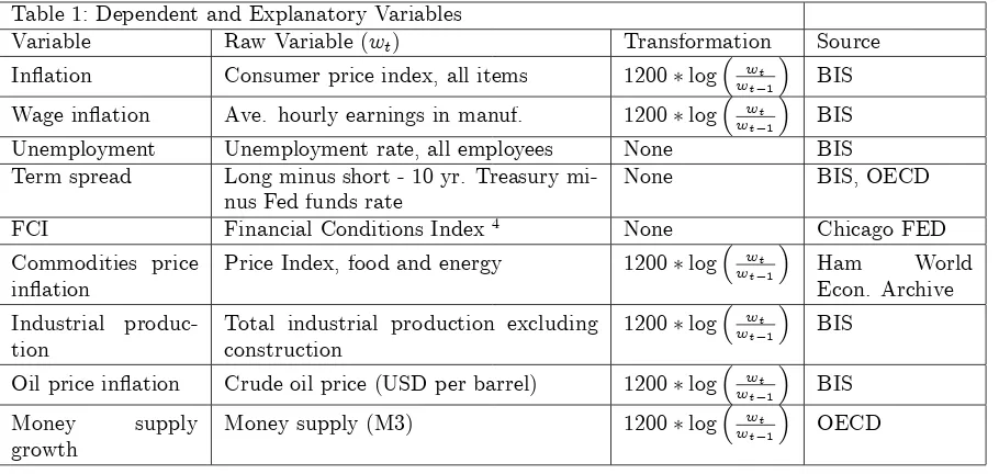
Table 1: Dependent and Explanatory Variables

Variable Raw Variable (wt) Transformation Source

In‡ation Consumer price index, all items 1200 log wt

wt 1 BIS

Wage in‡ation Ave. hourly earnings in manuf. 1200 log _wtwt

1 BIS

Unemployment Unemployment rate, all employees None BIS

Term spread Long minus short - 10 yr. Treasury mi-nus Fed funds rate

None BIS, OECD

FCI Financial Conditions Index4 _None _{Chicago FED}

Commodities price in‡ation

Price Index, food and energy 1200 log _wtwt

1 Ham World

Econ. Archive Industrial

produc-tion

Total industrial production excluding construction

1200 log _wtwt

1 BIS

Oil price in‡ation Crude oil price (USD per barrel) 1200 log _wtwt

1 BIS

Money supply

growth

Money supply (M3) 1200 log _wtwt

1 OECD

Corresponding to each of these variables, we produce a composite Google search variable. Of course, for any concept there are many potential Google search terms and there are di¤erent treatments of this in the literature. For ex-ample, Scott and Varian (2012) use 151 search categories.5 _{In this paper we use} a standardized procedure with the scope of minimizing the amount of judgement in the choice of variables. We start by searching for the name of the macro vari-able of interest and we collect the corresponding Google search volume. Along with this variable, the Google interface supplies a set of related terms. These are the most popular terms related to the search: Google chooses them in a me-chanical manner, by examining searches conducted by users immediately before and after. We fetch these related searches, and we repeat the procedure for each of them, …nding new terms. Only at this point some judgment is necessary. The related searches in Google are found automatically, therefore terms completely unrelated to economic concepts are removed manually. We could alternatively have chosen to limit our search to some speci…c Google category, but those are also de…ned automatically and remaining extraneous variables would have needed manual intervention. It is important, however, to note that variables are not eliminated on the basis of (expected) performance, but only when they

4_{Source: Chicago Fed. The indicator has an average value of zero and a standard deviation}

of one. Positive/negative numbers indicate tighter/looser than average …nancial conditions.

5_{Categories are aggregates of searches that are classi…ed by the Google engine as belonging}

(5)

are obvious mistakes (e.g. when searching for “spread” in relation to interest rates all results related to food are not retained). We also mechanically deleted all repeated terms, a frequent event when using the concept of “related” more than once. The remaining Google variables are attributed to the macro variable used to start the search.

Our …nal Google database is composed of 259 search results (see the Ap-pendix for a complete list). All series start at the beginning of 2004 and each volume search is separately normalized from 0 to 100. This normalization is done by …rst dividing the number of searches for a word by the total number of searches being done. This is done to avoid the issues that would arise due to the fact that, overall, the number of google searches is increasing over the sample period. The result is then normalized to lie between 0 and 100. Vari-ables searched with high volume have weekly frequency; less searched terms are supplied by the Google interface as monthly observations. Our research and the data to be forecasted are at most at monthly frequency, therefore we convert the weekly series by taking the last observation available for every month.

Thus, for each of the 9 macroeconomic variables in Table 1, we match a number of Google search variables. For each variable, we have, on average, over 20 Google search variables, unevenly distributed. To ensure parsimony, we adopt a strategy of averaging all the Google search variables to produce a single “Google variable” corresponding to each macroeconomic variable. Such a strategy works well, although other more sophisticated methods (e.g. using principal components methods) would be possible.

The 9 Google variables constructed in this fashion are plotted in Figure 1. The macroeconomic variables themselves are plotted in Figure 2. A compar-ison of each Google variable to its macroeconomic counterpart does not tend to indicate a close relationship between the two. There are some exceptions to this. For instance, the increase in Google searches related to unemployment matches up well with the actual unemployment rate, especially as the …nan-cial crisis occurs. But overall, the di¤erences are greater than the similarities. For instance, several of the Google search variables exhibit much less variation over time than their actual counterparts (e.g. the Google variables for wages, …nancial conditions and industrial production are all roughly constant over the sample). This suggests why regressions involving Google variables might not be good forecasting models for these macroeconomic variables. However, this does not preclude that the Google variables might be useful predictors at particular times. For instance, the Google variable for the term spread in general looks very di¤erent from the term spread itself. However, it does exhibit an increase in the run up to the …nancial crisis which matches the behavior of this variable at this point in time. Our multi-model, dynamic approach is well-designed to accommodate such features in a way which single regressions are not.

(6)

macroeco-2005 2010 0

50 100

Inflation

2005 2010

0 50 100

Wage Inflation

2005 2010

0 50 100

Unemployment

2005 2010

0 50 100

Term Spread

2005 2010

0 50 100

FCI

2005 2010

0 50 100

Commodity Price

2005 2010

0 50 100

Ind. Production

2005 2010

0 50 100

Oil Price

2005 2010

0 50 100

[image:6.612.170.519.244.530.2]

Money Supply

(7)

2005 2010 -20

-10 0 10

Inflation

2005 2010

-2 0 2 4 6 8

Wage Inflation

2005 2010

5 10

Unemployment

2005 2010

1 2 3

Term Spread

2005 2010

0 2 4

FCI

2005 2010

-200 -100 0 100

Commodity Price

2005 2010

-40 -20 0

Ind. Production

2005 2010

-200 0 200

Oil Price

2005 2010

0 10 20

[image:7.612.171.521.242.533.2]

Money Supply

(8)

nomic concept.6

3 Models

Each of our models involves using one of the macroeconomic variables as a de-pendent variable,yt, with the remainder of the macroeconomic variables being

included as potential explanatory variables, Xt. The Google variables

corre-sponding toXtwill be labelledZt. The Google variables are available weekly,

whereas the macroeconomic variables are available monthly. In our empirical work, we use the Google data from the last week of month t and, thus, Zt is

data which will be available at the end of the last week of montht. Of course, other timing conventions are possible depending on when nowcasts are desired.

3.1 Our Baseline: Regressions with Constant Coe¢ cients

A standard, one-step ahead regression model for forecastingytis:

yt=Xt0 1 +"t: (1)

Typically, the model would also include lags of the dependent variable and an intercept. All models and all the empirical results in this paper include these (with a lag length of 2), but for notational simplicity we will not explicitly note this in the formulae in this section.

We then add the Google regressors. We assume the following timing conven-tion: At the end of monthtor early in montht+ 1, we assumeythas not been

observed and, hence, we are interested in nowcasts of it. The Google search data for the last week of montht, Zt, becomes available. The other macroeconomic

variables are released with a time lag so that Xt 1 is available, but not Xt.

With these assumptions about timing, the following regression can be used for nowcastingyt early in montht+ 1

yt=Xt0 1 +Zt0 +"t: (2)

The results in this paper adopt this timing convention, but other timing conventions (e.g. nowcasting in the middle of a month) can be accommodated with minor alterations of the preceding equation (depending on the release date of the variables inXt).

3.2 TVP Regression Models, Model Averaging and Model

Switching with Google regressors

The regressions in the preceding sub-section have two potential problems: i) they assume coe¢ cients are constant over time which, for many macroeconomic

6_{Note that the macroeconomic variables and Google variables have di¤erent time spans}

(9)

time series, is rejected by the data (see, among many other, Stock and Watson, 1996) and ii) they may be over-parameterized since the regressions potentially have many explanatory variables and the time span of the data may be short.

An obvious way to surmount the …rst problem is to use a TVP regression model. TVP regression models (or multivariate extensions) are increasingly popular in macroeconomics (see, among many others, Canova, 1993, Cogley and Sargent, 2001, 2005, Primiceri, 2005, Canova and Gambetti, 2009, Canova and Ciccarelli, 2009, and Koop, Leon-Gonzalez and Strachan, 2009, and Chan et al, 2012). Our TVP regression model is speci…ed as:

yt = Wt t0 +"t (3)

t+1 = t+ t;

where, in our empirical work, we consider bothWt=Xt 1andWt= Xt0 1; Zt0

0

. Note thatWtde…ned in this way includes all information available for

nowcast-ingytat the end of montht. Furthermore, t are independentN(0; Qt)random

variables (also independent of"t). An advantage of such models is that they are

state space models and, thus, standard methods for estimating them exist (e.g. involving the Kalman …lter). However, a possible disadvantage is they can be over-parameterized, exacerbating the second problem noted above.

Before discussing the more innovative part of our modelling approach, we note that, in all of our models, we allow for time variation in the error variance. Thus,"tis assumed to be i.i.d. N 0; 2t , where 2t is replaced by an

Exponen-tially Weighted Moving Average (EWMA) estimate (see RiskMetrics, 1996 and West and Harrison, 1997 and note that EWMA is a special case of a GARCH model):

bt= bt 1+ (1 )b"tb"0t; (4)

whereb"tare the estimated regression errors. We set the decay factor, = 0:96

following suggestions in Riskmetrics (1996).

Due to over-parametrization concerns, there is a growing literature which uses model averaging or selection methods in TVP regressions. That is, in-stead of working with one large over-parameterized model, parsimony can be achieved by averaging over (or selecting between) smaller models. Thus, model averaging or model selection methods can be used to ensure shrinkage in over-parameterized models. With TVP models, it is often desirable to do this in a time-varying fashion and, thus, DMA or DMS methods can be used (see, e.g., Koop and Korobilis, 2012). These allow for a di¤erent model to be selected at each point in time (with DMS) or di¤erent weighs used in model averaging at each point in time (with DMA). For instance, in light of Choi and Varian (2011)’s …nding that Google variables predict better at some points in time than others, one may wish to include the Google variables at some times but not oth-ers. DMS allows for this. It can switch between models which include Google variables and models which do not, as necessary.

(10)

the DMA algorithm used in this paper, we will not provide complete details here. Instead we just describe the model space under consideration and the general ideas involved in the algorithm.

Instead of working with the single regression of the form (3), we have j = 1; ::; J TVP regression models, each of the form:

yt = Wt(j) (j) t +"

(j)

t (5)

(j) t+1 =

(j)

t +

(j) t ;

where "(_tj) is N 0; 2(_tj) and _t(j) is N 0; Q(_tj) . The W_t(j) contain di¤erent sub-sets of the complete setWtof potential explanatory variables. If we denote Sas the number of explanatory variables inWt(e.g. in TVP regressions which

do not include Google variables, then S = 8 since one of the macroeconomic variables in Table 1 will be the dependent variable and the remaining 8 will enter in lagged form as explanatory variables), then there areJ = 2S _{possible TVP}

regressions involving every possible combination of theSexplanatory variables. Unless S is small, it can be seen that the model space is huge. As discussed in Koop and Korobilis (2012), exact Bayesian estimation of this many TVP regression models (allowing for stochastic volatility in the errors) using Markov Chain Monte Carlo (MCMC) is computationally infeasible which motivates our use of EWMA and forgetting factor methods.

Within a single TVP regression model we estimate 2(t j)using EWMA

meth-ods (as described above) andQ(_tj) using forgetting factor methods. Forgetting factors have long been used in the state space literature to simplify estimation. Sources such as Raftery et al (2010) and West and Harrison (1997) describe forgetting factor estimation of state space models and we will not repeat this material here. Su¢ ce it to note that they involve choice of a scalar forgetting factor ₂ [0;1] and lead to estimates of (_tj) where observationsj periods in the past have weight j. An alternative way of interpreting is to note that it implies an e¤ective window size of ₁1 . With EWMA and forgetting factor methods used to estimate 2(_t j) and Q(_tj), all that is required is the use of the Kalman …lter in order to provide estimates of the states and, crucially for our purposes, the predictive density, pj(ytjW1:t; y1:t 1), where W1:t = (W1; ::; Wt)

andy1:t 1= (y1; ::; yt 1).

DMA and DMS involve a recursive updating scheme using quantities which we labelqtjt;j andqtjt 1;j. The latter is the key quantity: it is the probability

that modeljis the model used for nowcastingyt, at timet, using data available

at timet 1. The former updatesqtjt 1;j using data available at timet. DMS

involves selecting the single model with the highest value forqtjt 1;j and using

it for forecastingyt. Note that DMS allows for model switching: at each point

in time it is possible that a di¤erent model is used for forecasting. DMA uses forecasts which average over allj= 1; ::; Jmodels usingqtjt 1;jas weights. Note

that DMA is dynamic since these weights can vary over time.

(11)

qtjt;j=

qtjt 1;jpj(ytjW1:t; y1:t 1)

PJ

l=1qtjt 1;lpl(ytjW1:t; y1:t 1)

(6)

wherepj(ytjW1:t; y1:t 1)is the predictive likelihood (i.e. the predictive density

foryt produced by the Kalman …lter run for modelj evaluated at the realized

value foryt). The algorithm then uses a forgetting factor, , set to 0.99 following

Raftery et al (2010), to produce a model prediction equation:

qtjt 1;j =

q_t ₁_j_t ₁_;j

PJ

l=1qt 1jt 1;l

: (7)

Thus, starting withq0j0;j (for which we use the noninformative choice ofq0j0;j = 1

J for j = 1; ::; J) we can recursively calculate the key elements of DMA: qtjt;j

andqtjt 1;j forj= 1; ::; J.

3.3 DMA and DMS with Google Probabilities

Our …nal and most original contribution consists of using the Google variables not directly as regressors, but as providing information to determine which macroeconomic variables should be included at each point in time. The under-lying intuition is that the search volume might show the relevance of a certain variable for nowcasting at one point in time rather than a precise and signed cause-e¤ect relationship. Therefore even those Google searches showing little direct forecasting power as explanatory variables in a regression might be useful in selecting the explanatory variables of most use for nowcasting at any given point in time. Motivated by these considerations, we propose to modify the conventional DMA/DMS methodology as follows.

LetZt= (Z1t; ::; Zkt)0 be the vector of Google variables and remember that

we construct our data set so that each macroeconomic variable is matched up with one Google variable. Zit is standardized by Google to be a number

be-tween 0 and 100. Conveniently re-sized, this number can be interpreted as a probability.

Consider the same model space as before, de…ned in (5), with Wt=Xt 1.

For each of these models and for each time t we de…ne pt;j, which we call a

Google probability:

pt;j=

Y

s2Ij Zst

Y

s2I j

(1 Zst):

whereIj_{indicates which variables are in model}_j_{. For instance, if model}_j_{is the}

TVP regression model which contains lags of the third and seventh explanatory variables thenIj ₌_f₃_;₇_g_:_{In a similar fashion, we denote the explanatory}

vari-ables which are excluded from modelj byI j. It can be seen that

J

X

j=1

pt;j = 1

(12)

when internet searches on terms relating to the third and seventh explanatory variables are unusually high and it will be low when such searches are unusually low.

Our modi…ed version of DMA and DMS with Google model probabilities involves implementing the algorithm of Raftery et al (2010), except with the time varying model probabilities altered to re‡ect the Google model probabilities as:

qtjt 1;j =!

q_t ₁_j_t ₁_;j

PJ

l=1qt 1jt 1;l

+ (1 !)pt;j (8)

where ! can be selected by the researcher and 0 ! 1. If ! = 1 we are back in conventional DMA or DMS as done by Raftery et al (2010), if! = 0

thenpt;sreplacesqtjt 1;s in the algorithm (and, hence, only the Google model

probabilities are driving model switching). Intermediate values of!will combine the information in the Google internet searches with the Raftery et al (2010) data-based model probabilities.

It is worth noting that there exist other approaches which allow for model probabilities to depend upon explanatory variables such as we do with our Google model probabilities. A good example is the smoothly mixing regression model of Geweke and Keane (2007). Our approach di¤ers from these in two main ways. First, unlike the smoothly mixing regression model, our approach is dynamic such that a di¤erent model can be selected in each time period. Second, our approach avoids the use of computationally-intensive MCMC methods. As noted above, with2S _{models under consideration, MCMC methods will not be}

feasible unlessS, the number of predictors, is very small.

4 Nowcasting Using DMS and DMA with Google

Model Probabilities

4.1 Overview

(13)

We use mean squared forecast errors (MSFEs) to evaluate the quality of point forecasts and sums of log predictive likelihoods to evaluate the quality of the predictive densities produced by the various methods. Remember though, that our macroeconomic data is available from January 1973 through July 2012, but the Google data only exists since January 2004. In light of this mismatch in sample span, we estimate all our models in two di¤erent ways. First, we simply discard all pre-2004 data for all variables and estimate our models using this rel-atively short sample. Second, we use data back to 1973 for the macroeconomic variables, but pre-2004 we do not use versions of the models involving the un-available Google data. For instance, when doing DMA with!= 1₂ we proceed as follows: Pre-2004 we do conventional DMA as implemented in Raftery et al (2010) so thatqtjt 1;j is de…ned using (7). As of January 2004, however,qtjt 1;j

is de…ned using (8).7 _{Results using post-2004 data are given in Table 2 with} results using data since 1973 being in Table 3. In the former case, the nowcast evaluation period begins in September 2005, in the latter case in January 2004. In both cases, the nowcast evaluation period ends in July 2012. Our OLS and No-change benchmark approaches involve only one model and do not produce predictive likelihoods. Hence, only MSFEs are provided for these benchmarks which (to make the tables compact) are put in the column labelled DMA in the tables.

4.2 Discussion of Empirical Results

With 9 variables, two di¤erent forecast metrics and two di¤erent sample spans, there are 36 di¤erent dimensions in which our approaches can be compared. Not surprisingly, we are not …nding one approach which nowcasts best in every case. However, there is a strong tendency to …nd that DMA and DMS methods nowcast better than standard benchmarks and there are many cases where the inclusion of Google data s nowcast performance relative to the comparable ap-proach excluding the Google data. Inclusion of Google data in the form of model probabilities is typically (although not always) the best way of including Google data. It is typically the case that DMS nowcasts better than the comparable DMA algorithm, presumably since the ability of DMS to switch quickly be-tween di¤erent parsimonious models helps improving nowcasts. The remainder of this sub-section elaborates on these points, going through one macroeconomic variable at a time.

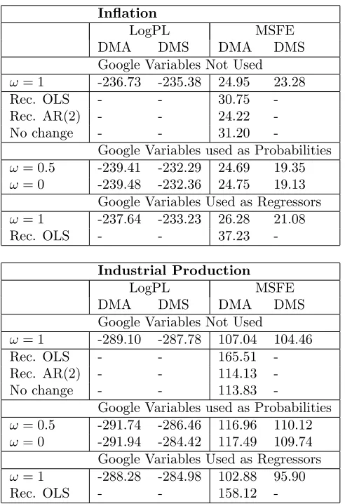
In‡ation. For in‡ation, we …nd DMS with ! = 0 or ! = 1₂ to produce the best nowcasts, regardless of data span or forecast metric. Note that both of these approaches uses Google probabilities. Doing DMS using Google variables as regressors leads to a worse nowcast performance. For instance, Table 2a shows that doing DMS using Google probabilities yields an MSFE of 19.13 but if DMS is done in the conventional manner using Google variables as regressors, the MSFE is 21.08, which is a fairly substantial deterioration. If the Google

7_{For the case where the Google variables are included as regressors, we only use post-2004}

(14)

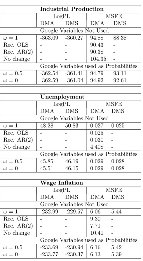
variables are simply used as regressors in a recursive OLS exercise, the MSFE deteriorates massively to 37.23. Similar results, where relevant, hold for the predictive likelihoods. In Table 2a, the best MSFE for an OLS benchmark model is 24.22 which also is much worse than DMS using Google probabilities. Industrial Production: As with in‡ation, there is strong evidence that DMS leads to nowcast improvements over benchmark OLS methods. However, evidence con‡icts on the best way to include Google variables. If we use only the post–2004 data, the MSFEs indicate the Google variables are best used as regressors (along with DMS methods). However, predictive likelihoods indicate that DMS with Google model probabilities nowcasts best. However, if we use data since 1973, MSFEs and predictive likelihoods both indicate that simply doing DMS using the macroeconomic variables nowcasts best. Hence, we are …nding strong support for the use of DMS, but a less clear story on how or whether Google variables should be used with DMS.

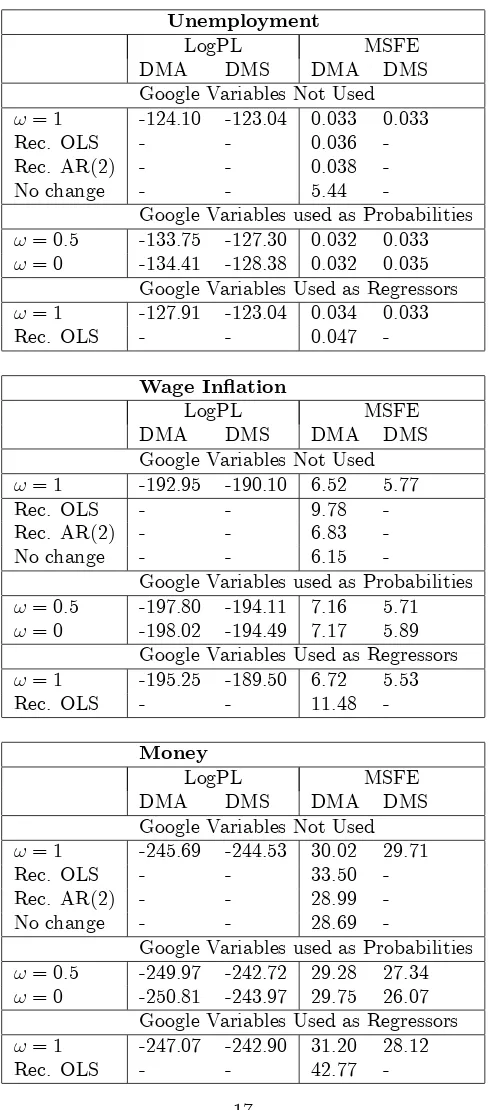
Unemployment: With the post-2004 data, MSFEs indicate support for our DMS approach using Google probabilities, but predictive likelihoods indicate a preference for using the Google variables as regressors (or not at all). When us-ing the post-1973 sample, predictive likelihoods also indicate support for DMS using Google probabilities. However, MSFEs indicate omitting the Google vari-ables leads to the best nowcasts, with conventional DMS and recursive OLS being the winning approaches according to this metric.

Wage in‡ation: This is a variable for which MSFE and predictive likeli-hood results are in accordance. For the post-2004 sample they indicate conven-tional DMS, using the Google variables as regressors, is to be preferred. How-ever, for the post-1973 sample, they indicate DMS using Google probabilities nowcasts best.

Money: The di¤erent measures of nowcast performance and sample spans also lead to a consistent story for money supply growth. In particular, DMS with Google probabilities nowcasts best, although there is some disagreement over whether!= 0or 1₂.

Financial Conditions Index: Using MSFEs, both sample spans indicate that DMS with Google data nowcasts best. Predictive likelihoods, though, show a con‡ict between whether the Google variables should be used as regressors (post-2004 data) or not included at all (post-1973 data).

Oil Price In‡ation: For this variable, both nowcast metrics and data spans indicate DMS with!= 0nowcasts best. This is the version of DMS which let the Google model probabilities entirely determine which model is selected at each point in time.

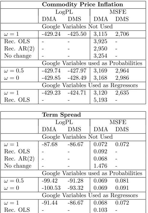
Commodity Price In‡ation: Using the post-2004 sample, we …nd the best performance using DMS with the Google variables being used as regres-sors. However, using the post-1973 sample we …nd the approaches including the Google model probabilities (either with!= 0or 1₂) to nowcast best.

(15)

also that this is one of the few variables where a benchmark approach does well. In particular, using the post-2004 sample, an AR(2) model nowcasts quite well (although it does not beat our DMS approach).

(16)

[image:16.612.184.430.145.504.2]

Table 2a: Nowcast Performance (post-2004 data)

In‡ation

LogPL MSFE

DMA DMS DMA DMS

Google Variables Not Used

!= 1 -236.73 -235.38 24.95 23.28

Rec. OLS - - 30.75

-Rec. AR(2) - - 24.22

-No change - - 31.20

-Google Variables used as Probabilities

!= 0:5 -239.41 -232.29 24.69 19.35

!= 0 -239.48 -232.36 24.75 19.13 Google Variables Used as Regressors

!= 1 -237.64 -233.23 26.28 21.08

Rec. OLS - - 37.23

-Industrial Production

LogPL MSFE

DMA DMS DMA DMS

!= 1 -289.10 -287.78 107.04 104.46

Rec. OLS - - 165.51

-Rec. AR(2) - - 114.13

-No change - - 113.83

!= 0:5 -291.74 -286.46 116.96 110.12

!= 1 -288.28 -284.98 102.88 95.90

(17)

-Table 2b: Nowcast Performance (post-2004 data)

Unemployment

LogPL MSFE

DMA DMS DMA DMS

!= 1 -124.10 -123.04 0.033 0.033

Rec. OLS - - 0.036

-Rec. AR(2) - - 0.038

-No change - - 5.44

!= 0:5 -133.75 -127.30 0.032 0.033

!= 1 -127.91 -123.04 0.034 0.033

Rec. OLS - - 0.047

-Wage In‡ation

LogPL MSFE

DMA DMS DMA DMS

!= 1 -192.95 -190.10 6.52 5.77

Rec. OLS - - 9.78

-Rec. AR(2) - - 6.83

-No change - - 6.15

!= 0:5 -197.80 -194.11 7.16 5.71

!= 1 -195.25 -189.50 6.72 5.53

Rec. OLS - - 11.48

-Money

LogPL MSFE

DMA DMS DMA DMS

!= 1 -245.69 -244.53 30.02 29.71

Rec. OLS - - 33.50

-Rec. AR(2) - - 28.99

!= 0:5 -249.97 -242.72 29.28 27.34

!= 1 -247.07 -242.90 31.20 28.12

[image:17.612.184.429.144.699.2]

(18)

-Table 2c: Nowcast Performance (post-2004 data)

Financial Conditions Index

LogPL MSFE

DMA DMS DMA DMS

!= 1 -53.22 -53.64 0.29 0.29

Rec. OLS - - 0.30

-Rec. AR(2) - - 0.32

-No change - - 0.45

!= 0:5 -58.92 -53.29 0.28 0.21

!= 0 -59.56 -54.56 0.28 0.21

Google Variables Used as Regressors

!= 1 -55.51 -51.56 0.32 0.26

Rec. OLS - - 0.48

-Oil Price In‡ation

LogPL MSFE

DMA DMS DMA DMS

!= 1 -484.51 -479.54 13,219 10,407

Rec. OLS - - 17,465

-Rec. AR(2) - - 11,253

-No change - - 12,185

!= 0:5 -481.39 -475.00 11,678 8,961

!= 0 -481.60 -474.71 11,857 8,555 Google Variables Used as Regressors

!= 1 -484.63 -479.72 13,241 10,415

[image:18.612.185.430.145.503.2]

(19)

-Table 2e: Nowcast Performance (post-2004 data)

Commodity Price In‡ation

LogPL MSFE

DMA DMS DMA DMS

!= 1 -429.24 -425.50 3,115 2,706

Rec. OLS - - 3,925

-Rec. AR(2) - - 2,950

-No change - - 3,254

!= 0:5 -429.74 -427.97 3,169 2,964

!= 0 -429.85 -428.49 3,168 2,986 Google Variables Used as Regressors

!= 1 -429.23 -424.71 3,120 2,635

Rec. OLS - - 5,193

-Term Spread

LogPL MSFE

DMA DMS DMA DMS

!= 1 -87.68 -86.67 0.072 0.072

Rec. OLS - - 0.092

-Rec. AR(2) - - 0.068

!= 0:5 -99.42 -91.28 0.069 0.081

!= 1 -91.44 -86.67 0.068 0.072

Rec. OLS - - 0.103

-Table 3a: Nowcast Performance (data since 1973)

In‡ation

LogPL MSFE

DMA DMS DMA DMS

!= 1 -293.11 -291.56 20.39 19.39

Rec. OLS - - 22.80

-Rec. AR(2) - - 24.16

!= 0:5 -293.71 -290.95 20.42 18.74

[image:19.612.184.430.159.513.2] [image:19.612.184.429.552.698.2]

(20)

[image:20.612.185.430.139.584.2]

Table 3b: Nowcast Performance (data since 1973)

Industrial Production

LogPL MSFE

DMA DMS DMA DMS

!= 1 -363.09 -360.27 94.88 88.38

Rec. OLS - - 90.43

-Rec. AR(2) - - 90.38

-No change - - 104.35

!= 0:5 -362.54 -361.41 94.79 93.11

!= 0 -362.59 -361.04 94.92 92.61

Unemployment

LogPL MSFE

DMA DMS DMA DMS

!= 1 48.28 50.83 0.027 0.025

Rec. OLS - - 0.025

-Rec. AR(2) - - 0.030

!= 0:5 45.85 46.19 0.029 0.028

!= 0 45.51 46.15 0.029 0.028

Wage In‡ation

LogPL MSFE

DMA DMS DMA DMS

!= 1 -232.99 -229.57 6.06 5.44

Rec. OLS - - 9.30

-Rec. AR(2) - - 7.71

!= 0:5 -233.69 -230.94 6.16 5.42

(21)

[image:21.612.183.429.143.551.2]

Table 3c: Nowcast Performance (data since 1973)

Money

LogPL MSFE

DMA DMS DMA DMS

!= 1 -294.56 -293.57 23.46 22.73

Rec. OLS - - 23.02

-Rec. AR(2) - - 23.34

!= 0:5 -293.99 -290.76 22.97 20.38

!= 0 -294.11 -291.24 23.07 20.92

Financial Conditions Index

LogPL MSFE

DMA DMS DMA DMS

!= 1 -28.63 -28.02 0.17 0.17

Rec. OLS - - 0.18

-Rec. AR(2) - - 0.20

-No change - - 0.36

!= 0:5 -31.71 -31.17 0.18 0.16

!= 0 -31.70 -31.15 0.18 0.16

Oil Price In‡ation Google Variables Not Used

!= 1 -610.18 -608.20 10,443 9,836

Rec. OLS - - 10,468

-Rec. AR(2) - - 9,740

-No change - - 10,957

!= 0:5 -609.54 -607.24 10,210 9,269

(22)

[image:22.612.183.427.141.430.2]

Table 3d: Nowcast Performance (data since 1973)

Commodity Price In‡ation

LogPL MSFE

DMA DMS DMA DMS

!= 1 -531.01 -528.20 2,230 2,080

Rec. OLS - - 2,198

-Rec. AR(2) - - 2,200

-No change - - 2,710

!= 0:5 -529.57 -528.19 2,230 2,079

!= 0 -529.64 -527.63 2,235 2,084

Term Spread

LogPL MSFE

DMA DMS DMA DMS

!= 1 2.980 6.239 0.062 0.056

Rec. OLS - - 0.109

-Rec. AR(2) - - 0.083

!= 0:5 2.374 6.785 0.062 0.053

!= 0 2.484 6.754 0.061 0.052

5 Further Discussion and Conclusions

The preceding discussion reveals a wide variety of …ndings. The following main conclusions emerge:

First, the inclusion of Google data leads to improvements in nowcast per-formance. This result complements the existing literature by showing that Google search variables are not only useful when dealing with speci…c disaggregate variables, but can be used to improve nowcasting of broad macroeconomic aggregates.

(23)

Third, Google probabilities make sense in a context where the economy is unstable, and are therefore particularly suited to deal with the recent crisis. However, their potential must be exploited with opportune tech-niques allowing for model change and parsimony. We compared di¤erent techniques responding to such requirements. DMS proved to be a par-ticularly good method for improving nowcast performance in the models we are dealing with, leading to substantial improvements over common benchmarks. It is also worth noting that DMS is a strategy which often nowcasts best, but even when it does not it does not go too far wrong. Our simple benchmarks, using OLS methods, sometimes also provide rea-sonable nowcasts but occasionally produce very bad nowcasts.

(24)

References

Artola, C. and Galan, E. (2012). “Tracking the future on the web: Construc-tion of leading indicators using internet searches,”Documentos Ocasionales No. 1203, Bank of Spain.

Askitas, N. and Zimmermann, K. (2009). “Google econometrics and unem-ployment nowcasting,” DIW Berlin, Discussion Paper 899.

Barreira, Nuno, Godinho, Pedro and Melo, Manuel, (2013), “Nowcasting unemployment rate and new car sales in south-western Europe with Google Trends”Netnomics, 14, issue 3, p. 129-165.

Canova, F. (1993). “Modelling and nowcasting exchange rates using a Bayesian time varying coe¢ cient model,”Journal of Economic Dynamics and Control, 17, 233-262.

Canova, F. and Ciccarelli, M. (2009). “Estimating multi-country VAR mod-els,”International Economic Review, 50, 929-959.

Canova, F. and Gambetti, L. (2009). “Structural changes in the US econ-omy: Is there a role for monetary policy?”Journal of Economic Dynamics and Control, 33, 477-490.

Carriere-Swallow, Y. and Labbe, F. (2011). “Nowcasting with Google trends in an emerging market,”Journal of nowcasting, doi: 10.1002/for.1252.

Chamberlin, G. (2010). “Googling the present,” U.K. O¢ ce for National Statistics Economic & Labour Market Review, December 2010.

Chan, J., Koop, G., Leon-Gonzalez, R. and Strachan, R. (2012). “Time varying dimension models,” Journal of Business and Economic Statistics, 30, 358-367.

Choi, H. and Varian, R. (2009). “Predicting initial claims for unemployment insurance using Google Trends,” Google Technical Report.

Choi, H. and Varian, R. (2011). “Predicting the present with Google Trends,” Google Technical Report.

Cogley, T. and Sargent, T. (2001). “Evolving post-World War II in‡ation dynamics,”NBER Macroeconomic Annual, 16, 331-373.

Cogley, T. and Sargent, T. (2005). “Drifts and volatilities: Monetary policies and outcomes in the post WWII U.S,”Review of Economic Dynamics, 8, 262-302.

D’Amuri, F. and Marcucci, J. (2009). “‘Google it!’ nowcasting the US unemployment rate with a Google job search index,” Institute for Economic and Social Research Discussion Paper 2009-32.

Dangl, T. and Halling, M. (2012). “Predictive regressions with time varying coe¢ cients,”Journal of Financial Economics,106, 157-181.

Fantazzini, D. & Toktamysova, Z. (2015). “Forecasting German car sales us-ing Google data and multivariate models,"”International Journal of Production Economics, Elsevier, vol. 170(PA), 97-135.

Geweke, J. and Keane, M. (2007). “Smoothly mixing regressions,”Journal of Econometrics, 138, 252-290.

(25)

Hellerstein, R. and Middeldorp, M. (2012). “Nowcasting with internet search data,”Liberty Street Economics Blog of the Federal Reserve Bank of New York, January 4, 2012.

Kholodilin, K., Podstawski, M. and Siliverstovs, S. (2010). “Do Google searches help in nowcasting private consumption? A real-time evidence for the US,” KOF Swiss Economic Institute Discussion Paper No. 256.

Koop, G. and Korobilis, D. (2012). “Forecasting in‡ation using dynamic model averaging,” International Economic Review, 53, 867-886.

Koop, G., Leon-Gonzalez, R. and Strachan, R. (2009). “On the evolution of the monetary policy transmission mechanism,”Journal of Economic Dynamics and Control, 33, 997–1017.

Koop, G. and Onorante, L. (2012). “Estimating Phillips curves in turbulent times using the ECB’s survey of professional nowcasters,” European Central Bank, working paper number 1422.

Koop, G. and Tole, L. (2013). “Forecasting the European carbon market,” Journal of the Royal Statistical Society, Series A, 176, Part 3, pp. 723-741.

McLaren, N. and Shanbhoge, R. (2011). “Using internet search data as economic indicators,” Bank of England Quarterly Bulletin, June 2011.

Nicoletti, G. and Passaro, R. (2012). “Sometimes it helps: Evolving predic-tive power of spreads on GDP,”European Central Bank, working paper number 1447.

Nymand-Andersen, P. and Pantelidis, E. (2018), “Nowcasting euro area car sales and big data quality requirements, ” Mimeo.

Primiceri. G. (2005). “Time varying structural vector autoregressions and monetary policy,”Review of Economic Studies, 72, 821-852.

Raftery, A., Karny, M. and Ettler, P. (2010). “Online prediction under model uncertainty via dynamic model averaging: Application to a cold rolling mill,”Technometrics, 52, 52-66.

RiskMetrics (1996). Technical Document (Fourth Edition). Available at http://www. riskmetrics.com/system/…les/private/td4e.pdf.

Scott, S. and Varian, H. (2012). “Bayesian variable selection for nowcasting economic time series,” manuscript available at

http://people.ischool.berkeley.edu/~hal/people/hal/papers.html.

Schmidt, T. and Vosen, S. (2009). “Nowcasting private consumption: Survey-based indicators vs. Google trends,” Ruhr Economic Papers, No. 155.

Stock, J. and Watson, M. (1996). “Evidence on structural instability in macroeconomic time series relations,”Journal of Business and Economic Sta-tistics,14, 11-30.

Suhoy, T. (2009). “Query indices and a 2008 downturn: Israeli data,” Bank of Israel Discussion Paper No. 2009.06.

West, M. and Harrison, J. (1997). Bayesian nowcasting and Dynamic Mod-els, second edition, New York: Springer.

(26)

Appendix: Categorization of Google Search Terms

Terms are grouped by category, categories are in bold.