Assessment of sub-Nyquist deterministic and random data sampling techniques for operational modal analysis

City, University of London Institutional Repository

Citation:

Monitoring, 16(5), pp. 630-646. doi: 10.1177/1475921717725029

This is the accepted version of the paper.

This version of the publication may differ from the final published

version.

Permanent repository link:

Link to published version:

Copyright and reuse: City Research Online aims to make research

outputs of City, University of London available to a wider audience.

Copyright and Moral Rights remain with the author(s) and/or copyright

holders. URLs from City Research Online may be freely distributed and

linked to.

City Research Online: http://openaccess.city.ac.uk/ [email protected]

Assessment of sub-Nyquist deterministic and random data sampling

techniques for operational modal analysis

Kyriaki GKOKTSI 1, Agathoklis GIARALIS 2

1 _{Dpt Civil Engineering (City, University of London)}

Northampton Square, EC1V 0HB - London (UK) [email protected]

2 _{Dpt Civil Engineering (City, University of London)}

Northampton Square, EC1V 0HB - London (UK) [email protected]

Key words: multi-coset sampling, sub-Nyquist sampling, compressive sensing, power

spectrum estimation, operational modal analysis, signal sparsity.

Abstract

This paper assesses numerically the potential of two different spectral estimation

approaches supporting non-uniform in time data sampling at sub-Nyquist average rates (i.e.,

below the Nyquist frequency) to reduce data transmission payloads in wireless sensor networks

(WSNs) for operational modal analysis (OMA) of civil engineering structures. This

consideration relaxes transmission bandwidth constraints in WSNs and prolongs sensor

battery life since wireless transmission is the most energy-hungry on-sensor operation. Both

the approaches assume acquisition of sub-Nyquist structural response acceleration

measurements and transmission to a base station without on-sensor processing. The response

acceleration power spectral density matrix is estimated directly from the sub-Nyquist

measurements and structural mode shapes are extracted using the frequency domain

decomposition algorithm. The first approach relies on the compressive sensing (CS) theory to

treat sub-Nyquist randomly sampled data assuming that the acceleration signals are

2

with significant magnitude). The second approach is based on a power spectrum blind

sampling (PSBS) technique considering periodic deterministic sub-Nyquist “multi-coset”

sampling and treating the acceleration signals as wide-sense stationary stochastic processes

without posing any sparsity conditions. The modal assurance criterion (MAC) is adopted to

quantify the quality of mode shapes derived by the two approaches at different sub-Nyquist

compression rates (CRs) using computer-generated signals of different sparsity and

field-recorded stationary data pertaining to an overpass in Zurich, Switzerland. It is shown that for

a given CR, the performance of the CS-based approach is detrimentally affected by signal

sparsity, while the PSBS-based approach achieves MAC>0.96 independently of signal sparsity

for CRs as low as 11% the Nyquist rate. It is concluded that the PSBS-based approach reduces

effectively data transmission requirements in WSNs for OMA, without being limited by signal

sparsity and without requiring a priori assumptions or knowledge of signal sparsity.

1 INTRODUCTION

The potential of using wireless sensor networks (WSNs) to facilitate field implementations

for operational modal analysis (OMA)1,2 of civil engineering structures has been widely

recognized in the past two decades3-6. In particular, WSNs enable cable-free acquisition and

transmission of response acceleration signals from linear vibrating structures excited by

broadband ambient dynamic loads. These signals are processed using OMA algorithms to

extract the structural dynamic properties (e.g., modal shapes and natural frequencies) which

are further used for condition assessment, design verification, and health monitoring

purposes1,2. In this context, WSNs reduce the up-front cost of OMA, compared to arrays of

wired sensors, while they allow for less obtrusive and more rapid sensor deployment, especially

in large-scale and/or geometrically complex civil engineering structures3,4.

Nevertheless, typical wireless sensors undertaking conventional uniform-in-time signal

3

maintenance cost of WSNs in long-term OMA deployments. The frequency of replacing

batteries ranges within few weeks to few months depending on various factors such as the

sampling frequency, the duration of each monitoring interval, and the on-sensor data

post-processing aiming for data compression3-8. The latter consideration reduces data transmission

payloads in order to (i) prolong battery life, since wireless transmission is the most power

consuming operation in a wireless sensor, and (ii) ensure the reliability of the monitoring

system, since the amount of data that can be transmitted within a WSN is subjected to

bandwidth limitations3,4.

To this end, it has been recently recognized that OMA relying on non-uniform in time data

sampling/acquisition techniques9-14 at sub-Nyquist rates (i.e., average sampling rates below an

assumed application-dependent Nyquist rate) is a viable alternative to off-line data

compression in reducing data transmission payloads. These techniques involve simultaneous

signal acquisition and compression at the sensor front-end. Therefore, requirements for

on-sensor data storage are relaxed while local on-board data processing before wireless

transmission is significantly reduced, or even by-passed. In this regard, most of measurement

post-processing and the associated computational burden is transferred from the sensors to the

server15_.

In this setting, this paper assesses the potential of two recent alternative spectral estimation

approaches relying on different non-uniform in time sub-Nyquist sampling schemes to extract

the mode shapes and associated natural frequencies of structures vibrating under operational

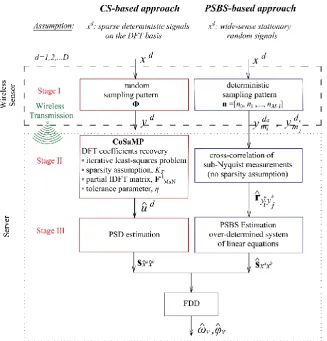
ambient loading. Figure 1 juxtaposes the steps involved in each of the two approaches. Both

the considered approaches involve the application of the standard frequency domain

decomposition (FDD) algorithm2 for OMA to the response acceleration power spectral density

(PSD) matrix pertaining to the sensors location. Further, in both approaches, the PSD matrix is

4

at average rates well below the Nyquist) without retrieving the traces of the acquired signals in

time domain. However, PSD matrix estimation is accomplished by making significantly

different assumptions for the attributes of the acquired signals and treating the compressive

measurements in a completely different manner.

Figure 1: Flowcharts of the two different sub-Nyquist sampling and spectral estimation approaches under comparison for frequency domain OMA.

Specifically, the approach proposed by O’Connor et al.9,10, delineated in the left flowchart

of Figure 1, is based on the theory of compressive sensing (CS)16-18. It assumes that structural

response acceleration signals are “sparse” on a pre-defined discrete Fourier transform (DFT)

basis. That is, they have a relatively small, K, number of DFT coefficients with magnitude

higher than an arbitrarily specified low threshold; by definition, if this threshold is set equal to

zero then the signals are termed K-sparse, otherwise they are termed K-compressible19. Relying

5

for sparse signal recovery19 to estimate the DFT coefficients of the response acceleration

signals by acquiring M>K random non-uniform in time measurements (CS-based sampling),

while the standard periodogram20 is used for the PSD matrix estimation. Notably, O’Connor et

al.9 achieved accurate mode shape estimation as well as appreciable savings in energy

consumption via the above approach using a WSN of five sensor nodes customized for

CS-based sampling to monitor an overpass in MI, USA. The sensors operated at up to 80% slower

average rate compared to a concurrently operating network of conventional wireless sensors

sampling uniformly in time at twice the assumed Nyquist rate. Given its successful field

implementation, the approach of O’Connor et al.9 is herein treated, among other approaches

11-13_{, as a paradigm of CS-based OMA using low-rate randomly sampled measurements with no}

on-sensor processing.

Importantly, in the above CS-based approach, as in all CS-based approaches for OMA9-13

and, more generally, for structural health monitoring8,21-24, the minimum average random

sampling rate for which quality signal recovery can be achieveddepends strongly on and is

limited by the actual sparsity/compressibility of the monitored response acceleration signals on

a pre-specified/assumed basis or frame25,26. At the same time, discrete-time versions of such

signals, as recorded in the field, may not be significantly sparse on a DFT basis8,9,23 _{partly due}

to unknown environmental excitation23 and partly due to spectral leakage27,28 associated with

the fact that the assumed grid of the DFT frequencies may not coincide with the (unknown)

resonant structural natural frequencies.

Outlined in the right flowchart of Figure 1, the second approach considered in this work was

recently developed by the authors14 _{to achieve frequency domain OMA using sub-Nyquist}

response acceleration measurements without imposing any signal sparsity conditions. In

particular, the method treats signals as realizations of an underlying wide-sense stationary

6

equivalently, the PSD matrix) through a power spectrum blind sampling (PSBS) step assuming

a deterministic periodic non-uniform-in-time sampling scheme known as multi-coset

sampling29-32.

From a practical viewpoint, it is emphasized that, contrary to the signal sparsity assumption

made by the CS-based approach, the stationarity signal assumption of the PSBS-based

approach does not limit the applicability of the method for OMA as the same assumption is

made by the FDD algorithm1,2_{. However, it is recognized that the PSBS-based approach cannot}

retrieve, by default, the time-histories of response acceleration signals. It, thus, can only be

applicable to structural health monitoring applications utilizing second-order random signal

statistics, which is the case of frequency domain-based OMA pursued in this work. In this

regard, the main contribution of this paper is the quantitative numerical assessment of the effect

of the signal sparsity assumption required by the CS-based approach to the achieved data

compression level for accurate modal properties estimation. This is accomplished by furnishing

novel results pertaining to the application of the two different sub-Nyquist spectral estimation

approaches in Figure 1 for two different case-studies. The first case study involve

computer-generated response acceleration signals of a white-noise excited simply supported steel beam

corrupted by additive Gaussian white noise. The second case study considers field recorded

response acceleration time-histories from an overpass in Zurich, Switzerland, monitored under

operational conditions33,34. In both case studies, performance is quantified in terms of the modal

assurance criterion (MAC)2 of mode shapes derived from a fixed number of compressed

measurements. Focus is given on gauging the sparsity requirements of the CS-based approach

and on numerically verifying that the accuracy of the PSBS-based approach is insensitive to

signal sparsity. Emphasis is also placed on quantifying the level of signal compression that can

be reached by the different compressive sampling schemes utilized in the two approaches,

7

is noted that the undertaken comparative numerical study is facilitated by the fact that both

approaches utilize the same frequency-domain OMA algorithm (FDD). Therefore, any

differences to the quality of mode shapes achieved by the competing methods can be attributed

to the different low-rate sampling schemes, and to the limitations posed by the associated

post-processing methods applied to the compressed measurements. Furthermore, the fairness of the

comparison in relation to up-front and/or operational monitoring costs is safeguarded by the

fact that neither of the approaches consider on-sensor data processing before transmission,

while no prior knowledge on the properties (i.e., the sparsity) of the acquired signals is assumed

available. The latter would theoretically benefit the CS-based approach but would require either

the use of an additional complementary network of wired sensors11 incurring additional

monitoring costs, or increased energy demands due to fast (conventional) uniform-in-time

sampling and heavy data post-processing on the wireless sensors21-24_{. Instead, this study}

assumes the availability of sensors that acquire and transmit signals directly in the compressed

domain supporting low-power WNSs9.

The remainder of the paper is organized as follows. Section 2 reviews briefly the adopted

CS-based approach9,10 shown in the left flow-chart of Figure 1. Section 3 outlines the

theoretical background of the PSBS-based spectral estimation approach14 _{shown in the right}

flow-chart of Figure 1. Sections 4 and 5 furnish comparative numerical results and discussion

pertaining to computer simulated and field recorded response acceleration measurements,

respectively. Finally, Section 6 summarizes concluding remarks.

2 COMPRESSIVE SENSING (CS)-BASED APPROACH

Consider a deterministic N-long discrete-time (response acceleration) signal x[n] N

being K-sparse/compressible on the DFT basis. The signal is expressed as

1 [ ] _{N N} [ ]

8

where F_{N N}1_  N N is the inverse discrete Fourier transform (IDFT) matrix, and u[n] Nis

the vector collecting the DFT coefficients of the considered signal having K entries with

significant magnitude, where K N. CS theory16-18 _{asserts that the information contained in}

this K-sparse signal x[n] can be retrieved in a robust manner from M non-uniform random

measurements y[m] M , where K<M N, and M/N is defined as the compression ratio (CR).

This is achieved by employing a measurement matrix Φ M N during sampling that satisfies

the so-called restricted isometry property (RIP)35, associated with the orthonormality level of

the columns of Φ. In this work, a Φ matrix populated with incoherent measurements of

zero-one entries that randomly selects M rows from the standard orthonormal IDFT matrix in Eq.

(1) is assumed, which defines the “partial” Fourier matrix F_{M N}1_  M N . To this end, the

compressed signal (i.e., vector collecting the M compressed measurements) y[m] is given by

1 1

[ ] _{N N} [ ] _{M N} [ ]

y m ΦF_ u n  e F_ u n e, (2)

where e is a vector representing measurement errors at the sensor. It is important to note that

the error term in Eq.(2) is added to the compressed measurements and does not influence the

sparsity level K of the signal x[n]. Such errors are treated by all standard CS sparse recovery

algorithms, as the one discussed below, by solving the so-called “noisy” sparse recovery

problem. However, in the numerical work of Section 4, noise is added to the signal x[n] in

Eq.(1). Such additive noise does influence the sparsity of the signal and cannot be rectified

during CS sparse recovery25.

Next, the dominant K DFT coefficients of x[n] are recovered from the compressed

measurements y[m] in Eq. (2) by using the iterative matching pursuit algorithm CoSaMP19.

This particular algorithm was used by O’Connor et al.9,10 for sparse recovery out of numerous

alternatives36 _{and is also adopted in the ensuing numerical work. CoSaMP takes as input the}

9

target sparsity level KT, which should be less than M/3, (i.e., KT<M/3), and a tolerance

parameter η. It returns a KT-sparse estimate ˆ[ ]u n of the K-sparse DFT spectrum u[n] that

satisfies the condition

2 /2 ₁ 2

1 ˆ

[ ] [ ] max , [ ] [ ]

T

K T

u n u n C u n u n

K         _   _  

 e ,

(3)

where _{/ 2}

 

T

K

u n is the optimal KT/2-sparse approximation of u[n], C is a constant, and a

p

is the

p norm of a. In each iteration, CoSaMP captures part of the energy of the target signal by

solving a least-squares problem involving the pseudoinverse of the matrix F_{M N}1_ in Eq. (2)19.

The extracted energy is subtracted from the target signal and in the next iteration the residual

signal becomes the target signal. This iterative process continues until any of the following

three stoppage criteria is met: (i) the relative residual signal energy between two iterations is

less than the tolerance η, or (ii)the total residual energy in the last iteration is smaller than η,

or (iii) a predefined maximum number of iterations is reached.

Following the OMA approach in O’Connor et al.9,10 illustrated in Figure 1 (left flowchart),

the above CS-based data sampling and sparse recovery steps are applied to an array of D

identical CS-based sensors. Each sensor d, d=1,2,…,D, compressively senses structural

response acceleration signals xd [n] at stage I, and wirelessly transmit the compressed

measurements yd [n] to a base station (server). The CoSaMP algorithm is then employed at

stage II to derive D estimates of the KT-sparse DFT coefficients, ûd [n], on the uniform Nyquist

grid. These coefficients can be used in a straightforward manner to obtain an estimate of the

PSD matrix in stage III using any standard spectral estimation technique assuming uniform

Nyquist sampling in time domain20. As a final step, the standard FDD algorithm is applied to

the PSD matrix obtained by the above CS-based approach to derive structural modal properties

10

It is important to note that the two critical parameters for robust and accurate structural

modes shape estimation (in the context of the above CS-based approach for OMA) are: (i) the

number of compressed measurements M, which should be of the order M ~ O(K∙log(N)) for

reasonably accurate sparse approximation of the DFT coefficients of field recorded response

acceleration signals, as reported by O’Connor et al. 9,10 ; and (ii) the target sparsity level KT

assumed in the sparse signal recovery step, which is associated with a trade-off between

reconstruction accuracy and computation complexity. Choosing a relatively large value of KT

(>>K) leads to unnecessarily high computational cost, as the latter is bounded by









 

  

T T

O K M N log x K M 19. On the antipode, a relatively small value of KT (<<K)

may lead to poor approximation of the Fourier coefficients of the vibration measurements and,

therefore, to low quality mode shape estimation. In practice, a range of different KT values

should be tested (off-line) to strike a good balance between accuracy and computational

complexity. It thus becomes obvious that both M and KT parameters depend on the signal

sparsity level K which is adversely affected by broadband environmental noise while it is

unknown, unless a priori knowledge becomes available through conventional uniform-in-time

sampling and signal processing11,23-25; a scenario that is not addressed in this paper. In the next

section, an alternative spectral estimation approach relying on low-rate (sub-Nyquist)

measurements is reviewed which does not depend on signal sparsity.

3 POWER SPECTRUM BLIND SAMPLING (PSBS)-BASED APPROACH

Consider now the sub-Nyquist spectral estimation approach shown in the right flowchart of

Figure 1. Let x(t) be a continuous in time t real-valued wide-sense stationary random signal (or

stochastic process) characterized in the frequency domain by the power spectrum Px(ω)

band-limited to 2π/T. It is desired to sample x(t) at a rate lower than the Nyquist sampling rate 1/Τ

(in Hz), and still be able to obtain a useful estimate of the power spectrum Px(ω). To this aim,

11

Nyquist sampled measurements x n[ ] N, is first divided into P blocks of N consecutive

samples, where N̅=N/P. From each block p={1,2,…P}, a number of M samples (M N ) is

selected at a deterministically pre-specified position which remains the same for all blocks.

The acquired number of samples further defines the associated CR given as M N/ . In this

manner, the multi-coset sampling strategy yields non-uniform-in-time deterministic N

-periodic samples; this is very different from the CS-based a-periodic random sampling briefly

reviewed in the previous section.

From a practical viewpoint, note that, as in the case of CS-based random sampling, there are

currently no commercially available sensors implementing sub-Nyquist multi-coset sampling

for structural health monitoring purposes. However, despite practical implementation

difficulties, efficient prototypes of compressive multi-coset samplers have been recently

developed 31,37.

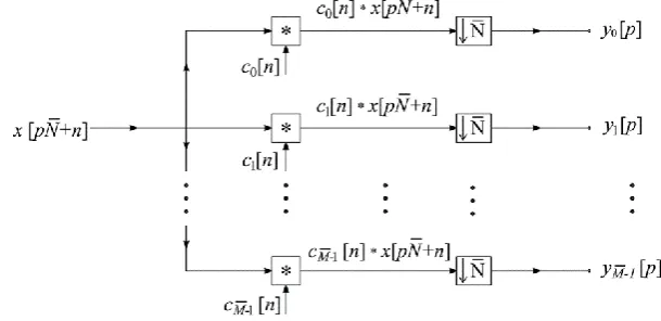
For illustration, Figure 2 shows a discrete-time model of an ideal multi-coset sampler30, in

which the p-th block of signal x[n] entersM channels and at each m channel (m= 0,1,…, M 1

), the input signal is convolved with an N -length sequence cm[n] and down-sampled by N.

Figure 2: Discrete-time model of the considered multi-coset sampling device30

The selection of M samples within each N-length block is given by the sampling pattern

T

0 1 1

[n n n_M ] 

12

latter arises naturally in the computation of the auto/cross correlation sequences of discrete

time signals, required for the blind recovery of the unknown power spectra of non-sparse

signals pertaining to any structure. Further, the multi-coset sampling pattern is governed by the

filter coefficients c n_m[ ] 1 for n nm, and c nm[ ]0 for n nm, where there is no

repetition in nm, i.e., nm_i nm_j,mimj. The output of the m-th channel of the considered

sampling device is given by the convolution operation y_m[ ]p 



indicated in Figure 2.

Importantly, the encoded information carried within the output signal y_m[ ]p (m= 0,1,…,

1

M  ) can be retrieved from the cross-correlation estimates among all M channels of the

adopted multi-coset sampler collectively. Thus, the difference set, S, is utilized to estimate the

correlation sequence of the signal x[n] at almost all lags within a given range, i.e. [-L, L],

outside which the correlation estimate takes on negligible values. In practice, the latter will

hold for some L depending on the level of damping of the monitored structural system.

Consider, next, an array of D identical multi-coset samplers with M channels each, the

cross-correlation function





y

, [ ] E [ ] [ ]

a b a b i j i j d d m m y y

r k  y l y lk _,

(4)

of the output signals a[ ]

i

d m

y l , b[ ] j

d m

y l can be computed for all mi, mj = 0,1,…,M1 channels

and da, db=1, 2,…, D devices (see also stage II in the right flowchart of Figure 1). In the above

equation, Ea{·} is the mathematical expectation operator with respect to a. Further, the

following relation holds14

c yayb = x xa b,

r R r (5)

where

2

(2 1) a b

M L D

y y

  

13

computed within the range (support) −L ≤ k ≤ L. Similarly, a b (2 1)

N L D

x x

  

r is a matrix

collecting the input cross-correlation sequences, [ ] E





d d x

x x

r k  x n x n k computed for

all da and db devices in the above range, and

2_{(2 1) (2 1)}

M L N L c

  



R is a sparse pattern correlation

matrix populated with the cross-correlations30 rc c_i, _j[ ] 



(5) defines an overdetermined system of linear equations which can be solved for a b

y y

r without

any sparsity assumptions, provided that R_c is full column rank. The latter is satisfied for

2

M N.

The unbiased estimator of the output cross-correlation function in Eq. (4) is then adopted,

   

1 min 0,

,

max 0,

1

ˆ [ ] a[ ] b[ ]

a b _{i j}

i j P p d d m m y y l p

r p y l y l p

P p      



in which P is the number of measurements that should be greater than L (PL) for perfect

power spectral recovery. Equation (6) is further used at stage III together with the DFT matrix,

(2 1) (2 1) (2 1)

N L N L L N

  

 

F , to obtain an estimate of the input cross-spectra s_{x x}a b at the discrete

frequencies ω=[0, 2π/(2L+1)N , … , 2π((2L+1)N -1)/(2L+1)N ] 32





ˆ a b _{L N c c c} ˆa b

x x y y



 

 

s F R W R R W r _.

(7)

In the above equation, W is a weighting matrix, and the superscript “−1” denotes matrix

inversion. The solution of Eq. (7) relies on the weighted least square criterion

2

c

ˆa b arg min ˆ a b a b , a b

x x

x x  _r y y  x x _W

r r R r _.

(8)

in which the weighted version of the Euclidean norm is given by || a ||2_WaTWa. Note that

14

estimator rˆ_{y y}a b, obtained from the compressed measurements of the D sampling devices, by

exploiting the sparse structure of R_c. As a final step, the PSD matrix in Eq. (7) is treated by

the FDD algorithm to extract mode shapes and natural frequencies14.

The critical parameters of the above briefly reviewed sub-Nyquist multi-coset sampling

PSBS approach for OMA are the number of cosets (or channels in Figure 2), M , and the value

of down-sampling N, subject to the two constraints M N and M2N . These constraints

are not very restrictive and will allow for spanning a good range of different CRs expressed by

the ratio M N/ . Therefore, once the values of M and Nare fixed, the weighting matrix W in

Eq.(7) and the sampling pattern n[n0 n1 nM1]T is determined by solving a

constrained least-squares optimization problem. Some further mathematical details on this

issue can be found in Tausiesakul and Gonzalez-Prelcic32.

4 NUMERICAL ASSESSMENT FOR SIMULATED SIGNALS OF DIFFERENT

SPARSITY LEVEL

4.1 Computer-simulated acceleration response signals

In this section, the effectiveness of the two sub-Nyquist spectral estimation approaches in

Figure 1 for OMA is assessed by considering simulated noisy structural acceleration response

signals obtained from the finite element model (FEM) in Figure 3. The modelled structure is

an IPE300-profiled simply supported steel beam with 5m length and flexural rigidity EI=

3

16.78 10 kNm2_{, which is assumed to be instrumented with a dense array of D=15 sensors}

measuring vertical accelerations along its length. The assumed sensor locations are shown with

white cross marks in Figure 3.

15

The adopted FEM is base-excited by a band-limited low-amplitude Gaussian white noise

force, observing a sufficiently flat spectrum in the frequency range up to 1000Hz. The

considered excitation is applied along the gravitational axis of the beam, having a duration of

4s and a time discretization step equal to 0.0005s.

Next, linear response history analysis is conducted, assuming a critical damping ratio of 1%

for all modes of vibration which is a reasonable value for a bare steel structure38. Vertical

response acceleration time-series are recorded at the 15 locations shown in Figure 3, with

Nyquist sampling rate at 2000Hz (i.e., 8000 “Nyquist samples” per signal). The acquired

acceleration responses are contaminated with additive Gaussian white noise expressed by the

signal-to-noise ratio SNR10 log ₁₀





x is the variance of the response

acceleration signal and 2

e is the noise variance. Two limiting SNR values are considered to

simulate response datasets associated with different sparsity levels: (i) a practically a noiseless

case with SNR=1020dB (i.e., the noise variance 2

e takes on a very small value close to zero),

yielding “high-sparse” signals on the DFT basis; and (ii) a noisy case with SNR=10dB (i.e., the

noise variance 2

e equals the 10% of the signal variance

2

_x) yielding “low-sparse” signals.

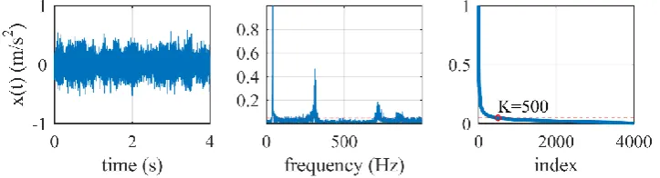
For illustration, Figure 4 plots a low-sparse acceleration response signal in time (left panel), its

single-sided magnitude Fourier spectrum normalized to its peak value (middle panel), as well

as the normalized magnitude Fourier coefficients sorted in descending order (right panel).

Figure 4: Typical noisy acceleration response signal with SNR=10dB; (left panel): time history; (middle panel): normalized single-sided Fourier spectrum magnitude; (right panel): Normalized magnitude Fourier coefficients in descending order. The red broken line

16

From the middle panel in Figure 4, it is readily observed that three dominant harmonics are

included in the signal on top of broadband noise, corresponding to the three first flexural mode

shapes of the beam. By inspection, a threshold is set in the right panel of Figure 4 (red broken

line) to indicate that the significant signal energy is captured from about 500 Fourier

coefficients and thus, a sparsity level of approximately K=500 may be assumed for the

considered noisy signals (see also O’Connor et al.9,10). It is emphasized that this threshold can

only be heuristically defined and is related to the concept of approximating a K-sparse signal

by a K-compressible signal provided that the coefficients of the latter on a given basis function

decay rapidly when sorted by magnitude. It is also important to clarify that the considered

CS-based spectral estimation approach assumes no prior knowledge on the actual sparsity level K,

but this is only reported here to facilitate the interpretation of the comparative results presented

in sub-section 4.3.

4.2 Sub-Nyquist sampling and power spectral estimation

The acceleration response signals generated as detailed above are next compressively

sampled at two different CRs of approximately 31% and 11% (i.e., 69% and 89% fewer samples

compared to the Nyquist samples) using the random CS-based sampling scheme of section 2

and the deterministic multi-coset sampling scheme of section 3. The adopted sampling

parameters are collected in Table 1. Specifically, a CR= 31% is achieved by multi-coset

samplers comprising M =5 channels, where each channel samples uniformly in time with a

rate N =16 times slower than the Nyquist rate. The adopted sampling pattern is n = [0 1 2 5

8]T. In this respect, only M=2500 samples are acquired by each sensor out of the N=8000

Nyquist samples. This exact pair of M, N values (i.e., M=2500, N=8000) is further used to

define the partial IDFT matrix F_{M N}1_  2500 8000 in Eq. (2) for the CS-based approach. The

effectiveness of the CS-based approach is assessed for various assumed (target) sparsity levels

17

are defined in a similar manner as above, such that the same number of compressed

measurements are acquired and transmitted by each sensor node for both the CS and the

multi-coset sampling schemes.

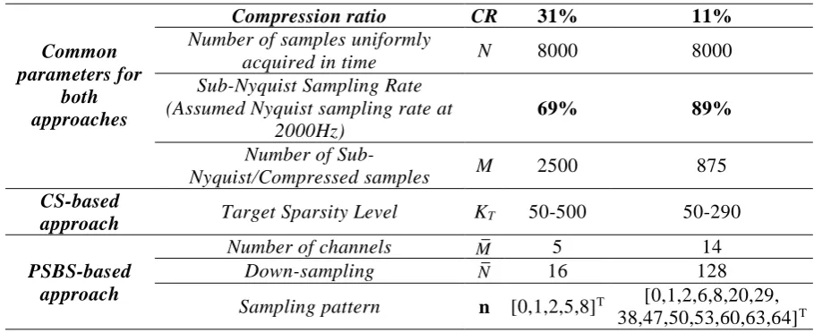
Table 1: Considered parameters for the CS-based and the PSBS-based approaches for OMA of the structure in Figure 3 for two different compression ratios.

Common parameters for

both approaches

Compression ratio CR 31% 11%

Number of samples uniformly

acquired in time N 8000 8000

Sub-Nyquist Sampling Rate (Assumed Nyquist sampling rate at

2000Hz)

69% 89%

Number of

Sub-Nyquist/Compressed samples M 2500 875

CS-based

approach Target Sparsity Level KT 50-500 50-290

PSBS-based approach

Number of channels M 5 14

Down-sampling N 16 128

Sampling pattern n [0,1,2,5,8]T [0,1,2,6,8,20,29,

38,47,50,53,60,63,64]T

Next, power spectral density matrices collecting estimates of the auto- and cross- power

spectra of the acceleration signals from the D=15 sensors are obtained using the two considered

spectral estimation methods in Figure 1 as detailed in sections 2 and 3. Specifically, for the

CS-based approach, the power spectral density functions are derived in three stages: (i)

compressive sensing using the matrix in Eq. (2); (ii) recovery of DFT coefficients using the

CoSaMP algorithm in Eq. (3) with an assumed target sparsity KT and stopping criteria

determined by tolerance η=10-8 and predefined maximum number of iterations set at 50; and

finally (iii) power spectrum estimation using the standard Welch’s modified periodogram20_.

The latter is applied to time-domain reconstructed acceleration responses, x̂[n], obtained by

application of the IDFT to the recovered signal coefficients, û[n], using Eq (1). To this end, the

“cpsd” built-in function in MATLAB® _{is adopted herein, in which the reconstructed signals}

are divided in eight segments with 50% overlap and windowed with a Hanning function.

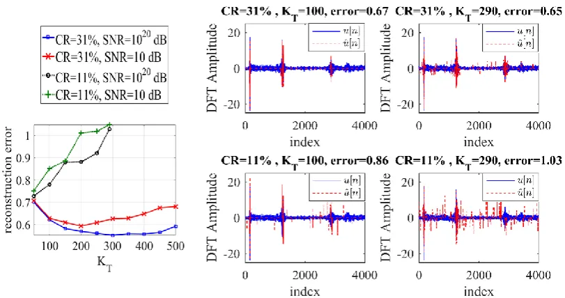
18 algorithm by plotting the CS reconstruction error,

2 ₂

ˆ[ ] [ ] [ ]

u n u n u n , as a function of the

target sparsity, KT,for both the examined CRs (i.e., 31% and 11%), at the two limiting SNRs

values (i.e., 1020dB, 10dB). For the case of CR=31%, smaller reconstruction errors are observed

at higher KT values, suggesting more accurate estimates as the number of recovered

measurements increases. This can be visualized at the top right panels of Figure 5 for CR=11%,

in which case the reconstruction error increases with KT. This rather poor reconstruction

performance is because an overly high compression level was assumed for which the relatively

small number of sub-Nyquist measurements y[m]in Eq. (2) do not retain sufficient information

of the structural response signals. Adopting, for example, the heuristic value of K=500 in Figure

4 (for the low-sparse signals with SNR=10dB), the required M value should be of the order of

K∙log(N)= 500∙log(8000)≈1950; however, only M=875 sub-Nyquist samples are acquired at

CR=11%, which are evidently too few. Along these lines, the bottom right panels of Figure 5

confirm that the assumption of higher KT values closer to the upper bound of M/3≈290 cannot

compensate for the insufficient number of compressed measurements, yielding spurious large

amplitudes in the recovered DFT coefficients that increases the reconstruction error and

adversely affects the accuracy of the obtained modal estimates, which will be presented in the

next sub-section. Similar conclusions have also been reported by O’Connor et al.9,10.

Moving to the PSBS-based approach, the PSD matrix is estimated through the following

three stages: (i) multi-coset sampling based on the sampling pattern in Table 1; (ii)

cross-correlation estimation applied to the compressed measurements as in Eq. (6); and (iii) power

spectrum estimation using Eq. (7). The recovered PSD estimates are illustrated in Figure 6 (red

curve) for the two adopted CRs at 31% (left) and 11% (right), respectively, considering the

low-sparse dataset. For comparison, Figure 6 also plots the pertinent PSD curves obtained from

the standard Welch’s modified periodogram at Nyquist rate (black curve), and reports the mean

19

found for lower CRs (left panel), which increases the MSE value. Nonetheless, the spectral

peaks are well captured from the PSBS approach in both amplitude and shape even for

CR=11%, which is essential for accurate modal identification.

Figure 5: Signal reconstruction error of CoSaMP algorithm versus the target sparsity level KT(left);

original and reconstructed DFT coefficients at CR={31%,11%}, KT={100, 290} for

SNR=10dB (right).

Figure 6: PSBS spectral recovery and MSE for the low-sparse response accelerations (SNR=10 dB) at CR=31% (left) and CR=11% (right).

4.3 Mode shapes estimation

The FDD algorithm is lastly applied to the PSD matrices obtained as detailed above to

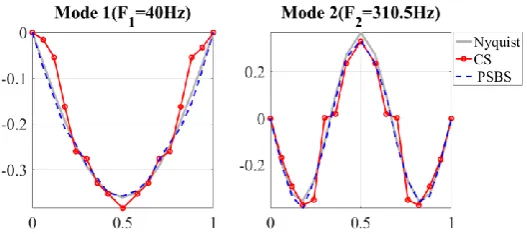
extract the modal properties of the beam in Figure 3. For illustration, Figure 7 presents all three

excited mode shapes derived from the noisy (i.e., lower-sparsity) measurements, as extracted

from the two different approaches (CS-based for KT=290 and PSBS-based) for CR=31%. In

20

third mode is not detectable at this low CR. For comparison, Figure 7 and 8 plot further the

mode shapes obtained by application of the FDD to the conventionally (Nyquist) sampled

measurements, considering the Welch periodogram20 with the same settings as detailed in the

previous sub-section. From a qualitative viewpoint, it is observed that both sub-Nyquist

approaches perform well for CR=31% in capturing the shape and relative amplitude of the

modal deflected shapes compared to the conventional approach, with the PSBS-based method

being slightly more accurate. For higher signal compression at CR=11%, the PSBS-based

method clearly outperforms the CS-based method.

Figure 7: Mode shape estimation for CR=31%, SNR=10dB (low-sparse signals) and target reconstruction sparsity KT=290 for the CS-based approach

Figure 8: Mode shape estimation for CR=11%, SNR=10dB (low-sparse signals) and highest possible target reconstruction sparsity KT=290 in the CS-based approach

To quantify the level of accuracy for the extracted mode shapes, the modal assurance

criterion (MAC)2

2 2

2 T

2 2

ˆ ˆ

( , )

ˆ

   

 



MAC

(9)

21

by means of the FDD algorithm from compressed (sub-Nyquist) and Nyquist samples,

respectively, with

2

 denoting the ₂ norm of φ. The normalized inner product in Eq. (9)

yields a scalar value within the range of [0, 1] and values of 0.9 and higher suggests acceptable

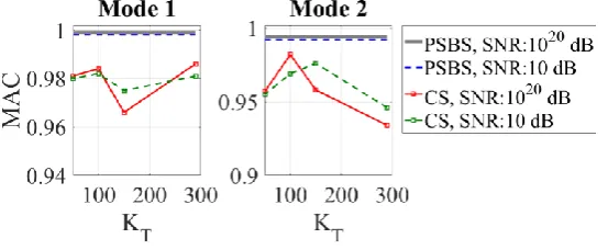
overall similarity/proximity between the ˆ and φ vectors. Figure 9 and 10 plot the computed

MAC values with respect to the assumed target sparsity KT for both the relatively high-sparse

(SNR=1020dB) and low-sparse (SNR=10dB) signals for CRs at 31% and 11%, respectively.

Figure 9: MAC versus reconstruction sparsity level KT, obtained from the two considered

approaches, PSBS-based and CS-based FDD, for CR= 31% and SNR={1020,10}dB

Figure 10: MAC versus reconstruction sparsity level KT, obtained from the two considered

approaches, PSBS-based and CS-based FDD, for CR= 11% and SNR={1020,10}dB The above figures show that for both sparsity levels, the PSBS-based approach outperforms

the CS-based approach for the same number of acquired (and wirelessly transmitted)

sub-Nyquist measurements regardless of the adopted target sparsity KT value. Specifically, the

PSBS-approach can accurately retrieve the modal deflected shapes yielding MAC values close

to unity. Notably, the PSBS method does not rely on sparsity assumptions, and therefore the

obtained MAC values are not functions of KT. Still, Figure 9 shows that the CS-based approach

22

assumed KT value. Importantly, for CR=31% higher accuracy is achieved for higher KT values

(note also the decreasing trend in the reconstruction error curve in Figure 5), but this comes at

the cost of higher computational demands in the signal reconstruction step. However, this is

not the case for CR=11% and for the second and less excited mode shape in Figure 10, where

the accuracy deteriorates yielding lower MAC values with increasing KT. This rather

unfavorable condition can be explained through Figure 5, where it is numerically shown that

higher CS reconstruction errors occurs at larger KT values for CR=11%, having a profound

impact on the accuracy of the obtained CS modal results. In this case, if a priori knowledge of

the signal sparsity was known11,21-24, then one should normally opt to increase the average

random sampling rate (i.e., obtain a larger number of measurements, M, within the same time

frame). Nevertheless, the signal agnostic PSBS approach is capable to extract structural mode

shapes associated with the local peaks of the spectrum even for CR=11% and signals with

lower sparsity (at SNR=10dB) as long as they are not completely “buried” in noise. For

instance, the right panel of Figure 6 reveals that the recovered PSBS-PSD at CR=11% and

SNR=10dB exhibits attains relatively large amplitudes close to the 3rd spectral peak, which

hinders the extraction of the associated vibrating mode of the beam in Figure 3.

As a final remark, it is noted that both the adopted sub-Nyquist methods yield fairly accurate

natural frequency estimates in all considered cases (error is less than 1% compared to the

conventional approach at Nyquist rate).

5 NUMERICAL ASSESSMENT FOR FIELD-RECORDED SIGNALS

5.1 The Bärenbohlstrasse bridge case-study and pre-processing of recorded data

Further to the previous comparison and along similar lines, the effectiveness of the two

considered spectral estimation approaches of Figure 1 is herein assessed against field recorded

data from an existing bridge, namely the Bärenbohlstrasseoverpass in Zurich, Switzerland33,34,

23

width, while it is almost symmetric along the longitudinal direction. It consists of a solid

prestressed-slab with two equal-length spans of 14.75m each. The deck is supported, via steel

bearings, in all directions at mid-span and in one of the abutments. The second abutment

supports the deck only in the vertical and transverse directions. The bottom face of the deck

was permanently instrumented for the 12-month period of 12th July 2013 to 26th July 2014 by

a network of 18 tethered sensors measuring vertical response acceleration signals at an hourly

basis. Measurements were acquired at the sampling rate of 200Hz (T=0.005s) for

approximately 10min per hour. A photo of the bridge and a sketch of the sensors layout is

shown in Figure 11. Further details regarding the bridge, the sensors installation and data

acquisition can be found in Spiridonakos et al.33 and in Chatzi and Spiridonakos34.

Figure 11: Bärenbohlstrasse bridge in Zurich, Switzerland (image reused from Spiridonakos et al 33) (left) and layout of the 18 sensors recording vertical acceleration responses under ambient

excitation (right).

In this study, a dataset of 18 vertical acceleration response signals is used, recorded on

19/06/2014 between 15:08:54 and 15:17:51, comprising 107460 samples per sensing location,

being conventionally (i.e., uniformly) sampled at 200Hz. The considered dataset pertains to

ambient wind and traffic dynamic loads that sufficiently excite the first few modes of the

monitored bridge. These raw signals acquired by the tethered sensor network in Figure 11 are

pre-processed as follows. Firstly, baseline adjustment is applied to the raw data to remove the

mean value and any potential low-frequency trend within each acceleration response signal.

Next, a 4th_{-order Butterworth band-pass filter is employed within the frequency range [0.15,}

24

adjusted and band-pass filtered) obtained from the sensor #13. Further, its magnitude Fourier

spectrum normalized to its peak value is plotted in the middle panel of Figure 12 for the

frequency range [0, 20] Hz, within which the first four modes of the vibrating bridge lie33.

Lastly, the right panel of Figure 12 plots the normalized magnitude Fourier coefficients sorted

in descending order. On the last plot, a heuristically selected threshold at 5% of the peak Fourier

spectrum magnitude (red broken line) is shown, indicating that the significant signal energy is

captured from approximately 10000 Fourier coefficients. Thus, the actual sparsity level of the

considered field recorded signals is roughly K≈10000. As previously discussed, though, no

such information would be available from the low-rate data acquisition using the two

sub-Nyquist spectral estimation approaches of Figure 1, but it is only reported to inform the

comparison of the OMA results discussed in the following sub-section.

Figure 12: Typical acceleration response signal measured at sensor #13; (left panel): time history;(middle panel): Normalized Fourier spectrum magnitude within the frequency range

of [0, 20] Hz; (right panel): Normalized magnitude Fourier coefficients in descending order. The red broken line signifies an arbitrary threshold at normalized Fourier spectrum

of 0.05.

Given that the PSBS-based spectral estimation approach anticipates signal stationarity, the

standard non-parametric Reverse Arrangement method Error! Reference source not found. _{is further}

applied on the considered acceleration response dataset to statistically test the stationarity

hypothesis, which is confirmed at the 95% confidence level.

5.2 Mode shapes estimation of the Bärenbohlstrasse bridge

The same steps detailed in sub-sections 4.2 and 4.3 (see also Figure 1) are herein taken to estimate

25

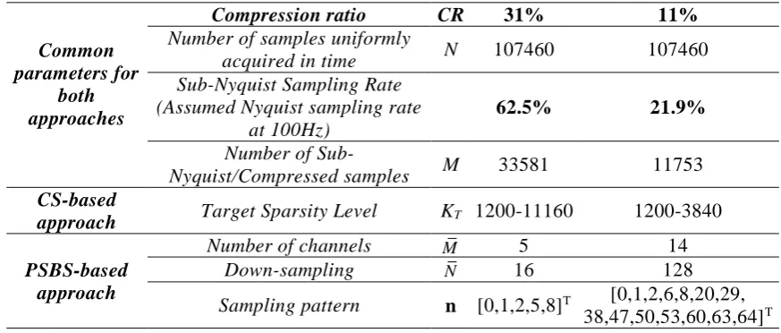
band-pass filtered) field recorded acceleration responses. Table 2 collects the parameters adopted

for the random CS-based and the deterministic multi-coset sampling at the same two CRs considered

before (i.e., 31% and 11%). Table 2 also reports the sub-Nyquist sampling rates achieved by the

adopted CRs based on the maximum cut-off frequency of the filtering operation at 50Hz, which

pertains to an assumed Nyquist sampling rate at 100Hz.

Table 2: Considered parameters for the CS-based and the PSBS-based approaches for OMA of the structure in Figure 11 for two different compression ratios.

Common parameters for

both approaches

Compression ratio CR 31% 11%

Number of samples uniformly

acquired in time N 107460 107460 Sub-Nyquist Sampling Rate

(Assumed Nyquist sampling rate at 100Hz)

62.5% 21.9%

Number of

Sub-Nyquist/Compressed samples M 33581 11753

CS-based

approach Target Sparsity Level KT 1200-11160 1200-3840

PSBS-based approach

Number of channels M 5 14

Down-sampling N 16 128

Sampling pattern n [0,1,2,5,8]T [0,1,2,6,8,20,29,

38,47,50,53,60,63,64]T

Further, Table 2 presents the range of different KT values (<M/3) considered in the CS-based

approach, which are directly related to the algorithmic trade-off between accuracy and

complexity. The latter reflects on the required running time of the CS signal reconstruction

algorithm for various KTvalues. As an example, Figure 13 plots the off-line computational time

required by the CoSaMP algorithm to recover the 18 bridge acceleration responses from the

acquired compressed measurements at CR=31% and 11% (left and right panel in Figure 13,

respectively). From this figure, it is readily observed that the CS computational cost

exponentially increases with KT. For comparison, Figure 13 also depicts the running time of

the PSBS-based approach (broken line) associated with the 18x18 spectral matrix estimation

detailed in Eqs. (6) and (7). All reported numerical work was performed on a quadcore Intel

26

Figure 13: Total running time for off-line signal and power spectral recovery required by the CS-based and the PSBS-CS-based approach, respectively, versus reconstruction sparsity level for

CR=31% (left) and CR=11% (right)

As a final step, the standard FDD algorithm is applied to the PSD matrices estimated by the

CS-based and the PSBS-based spectral estimation approaches reviewed in sections 2 and 3,

respectively, to extract the bridge mode shapes. For illustration, Figure 14 plots the first four

mode shapes of the considered bridge corresponding to two bending (modes 1 and 2) and two

rotational (modes 3 and 4) vibrating modes. They are obtained from the standard FDD method

using: (1) the 18 conventionally acquired signals, each comprising N=107460 samples (top

panels); (2) the CS-based approach for CR=11% and KT=3840; and (3) the PSBS-based

approach for CR=11% (lower panels).

From a qualitative inspection of these mode shapes, it can be deduced that both the

sub-Nyquist methods can adequately capture the shapes of the modal responses as estimated from

the uniformly sampled dataset. However, non-negligible differences are observed between the

conventional FDD and the CS-based approach, especially for the 2nd and the 4th vibrating

27

Figure 14: Mode shape estimation using: the conventional FDD (top); the CS-based approach for

CR=11% and target reconstruction sparsity KT=3840 (middle); the PSBS-based approach

for CR=11% (bottom)

To quantify the level of similarity between mode shapes obtained from the conventionally

sampled dataset and from the sub-Nyquist sampled acceleration responses, the MACin Eq. (9)

is plotted in Figure 15 and Figure 16 for the two considered CRs, respectively, as a function of

the assumed target sparsity KT for the CS-based (solid blue curve) and for the PSBS-based (red

broken line) approaches.

Figure 15: MAC versus reconstruction sparsity level KT, obtained from the two considered

28

Figure 16: MAC versus reconstruction sparsity level KT, obtained from the two considered approaches (i.e., PSBS-based and CS-based FDD) for CR= 11%.

It is confirmed that the PSBS-based method outperforms in accuracy the CS-based

approach, yielding higher MAC values in most of the cases considered. More importantly, the

PSBS-based approach provides mode shapes exhibiting nearly unit MACs, even in the case of

CR=11%(i.e., using almost 90% fewer measurements from the traditionally acquired signals)

without the need to assume a target sparsity level. On the antipode, the CS-based approach is

considerably affected by the assumed KT values. In fact, for the smaller compression level

considered (CR=31%), better accuracy is achieved for larger KT values for all mode shapes, at

the expense of higher computational cost during the sparse recovery step (see Figure 13).

However, such monotonic trends of MAC with KT are not confirmed for all the mode shapes

for the case of CR=11% in Figure 16, while the 2nd and 4th modes are not satisfactorily

estimated regardless of the KT value (i.e., MAC values lying below 0.9 are commonly used as

a practical criterion for rejecting mode shapes as inaccurate). As discussed before, this poor

performance of the CS-based approach is related to the underlying level of sparsity of the

acquired signals with respect to the number of compressed measurements, M, assumed.

29

(see the right panel of Figure 12), the number of compressed measurements that provides

reasonably accurate signal recovery results should be in the order of M ≈ K∙log(N) ≈

10000∙log(107460) ≈50000 (see also O’Connor et al.9,10_{). In this respect, the unsatisfactory}

performance of the CS-based approach for CR=11% can be attributed to the fact that the

number of compressed measurements (M=11753) randomly taken to achieve CR=11% is

significantly lower from the above assumed K∙log(N) value, which, apparently, is not the case

for CR=31% corresponding to about three time more measurements (M=33581). Remarkably,

it appears that the performance of the PSBS approach in terms of MAC values is almost

insensitive to CR. Nevertheless, it was deemed prudent not to consider lower CR values in this

numerical assessment, since this would require a large number of cosets (M >14) or parallel

channels in Figure 2 to satisfy the theoretical constraint of M2 N , as discussed in Section

3. In fact, one may note that even the consideration of M 14channels may be unrealistic in

practice. However, this is a setting that has been used before in pertinent theoretical

studies14,30,32, while recent advancements in the hardware implementation of multi-coset

samplers provide CRs independently of the number of interleaved ADCs37_.

As a final remark, it is expected that the gains to the CR achieved by the PSBS approach

compared to the CS-based approach in accomplishing quality OMA estimates, as those

reported above, would reflect analogously to energy savings in WSNs7,9_{. This is because}

wireless data transmission is by far the most power-hungry operation in wireless sensors, being

directly related to the amount of data, M, transmitted from each sensor in the considered setting.

Further, higher gains in the overall energy-efficiency will be achieved for larger WSN

deployments9. However, we refrain from reporting any particular estimate for the anticipated

energy savings since these would depend on several parameters such as the WSN topology, the

utilized wireless communication protocol, and the energy requirements of the multi-coset

multi-30

coset sampling which is an open area of research in the sensors community and lies beyond the

scope of this work.

6 CONCLUDING REMARKS

The performance of a CS-based approach vis-a-vis a PSBS-based approach for spectral

estimation relying on sub-Nyquist random and deterministic multi-coset sampling schemes,

respectively, has been numerically assessed in undertaking OMA. Both the approaches aim to

reduce data transmission payloads facilitating reliable and cost-efficient long-term OMA via

WSNs. This is accomplished by considering compressed structural acceleration responses

acquired at sub-Nyquist rates and wirelessly transmitted to a base station without any local

on-sensor data processing. The adopted approaches estimate the PSD matrix of the acceleration

signals by operating directly to the sub-Nyquist/compressed measurements at the base station.

Then, the standard FDD algorithm for OMA is applied to the estimated PSD matrix to extract

structural mode shapes.

The quality of mode shapes obtained from structural response acceleration signals

compressed at 31% and 11% below the Nyquist sampling rate (i.e., CR= 31% and 11%) using

the two considered approaches have been quantified through the MAC with respect to mode

shapes extracted from Nyquist sampled acceleration signals. For this purpose, two different

sets of acceleration signals have been considered. The first set was generated through linear

response history analysis applied to a white-noise excited finite element model of a simply

supported steel beam. Additive white Gaussian noise was considered at SNR=10dB to produce

a suite of relatively low-sparse acceleration signals in the frequency domain, aiming to gauge

the influence of signal sparsity to the performance of the considered approaches vis-à-vis the

high-sparse noiseless signals. The second dataset was acquired from an array of 18 tethered

sensors deployed onto a particular overpass in Zurich, Switzerland open to the traffic. Pertinent

31 compressive sampling.

It has been numerically shown and theoretically justified, that, for a given sub-Nyquist

sampling rate, the capability of the CS-based approach to extract faithful estimates of the mode

shapes depends heavily on the target sparsity level, KT, which needs to be assumed in the CS

signal reconstruction step. It has also been demonstrated that the accuracy of the CS-based

approach improves at larger KT values at the cost of higher computational effort reflected on

the increased required runtime of the adopted CS sparse signal recovery algorithm. However,

no increase to the assumed KT value can compensate for the acquisition of an excessively small

number of compressed measurements which is the case for CR=11% for all the sets of

acceleration signals considered in this work. In this regard, it is concluded that conservative

compression ratios should be adopted in using the CS-based approach to ensure acceptable

quality of modes shapes, especially in the case where no prior knowledge on the acceleration

signal sparsity is available.

On the antipode, it was numerically shown that the PSBS-based approach, which treats

response acceleration signals as wide-sense stationary stochastic processes without imposing

any signal sparsity conditions, performs equally well and consistently better than the CS-based

approach in extracting mode shapes for all the herein considered sets of compressively sampled

acceleration signals. In fact, the PSBS-based approach yields MAC>0.96 even for the

low-sparse signals contaminated with white noise at SNR=10dB and for low sampling rates at

CR=11% (i.e., 89% below the Nyquist rate).

Overall, the herein furnished numerical data demonstrate that the inherent signal agnostic

attributes of the PSBS-based approach renders this method more advantageous compared to

the CS-based approach in OMA applications where high signal compression levels are desired

to address sensor power consumption and wireless bandwidth transmission limitations. Further,

32

and power spectral estimates) and extracts structural modal properties directly from the

acquired compressed data yielding computationally efficient OMA. It is recognized, though,

that the PSBS approach is strictly a spectral estimation method that does not return the

monitored signals deterministically in time domain. This limits the use of PSBS to structural

health monitoring applications where time-domain signal monitoring is not of essence as in the

case of frequency domain based OMA. Still, further research is warranted to assess the

potential of the considered PSBS-based spectral estimation approach in actual field

deployments. Such an assessment necessitates the development of custom-made wireless

sensors featuring either multi-coset samplers at the hardware level or, alternatively, efficient

algorithms for off-line on-sensor multi-coset sampling. These aspects are left for future work

by the authors.

AKNOWLEDGEMENTS

This work has been funded by EPSRC in UK, under grant No EP/K023047/1. The first

author further acknowledges the support of City, University of London, through a PhD

studentship. The authors are indebted to Prof. Eleni Chatzi and to Dr Vasileios Dertimanis for

providing the field recorded data from the BärenbohlstrasseBridge used in Section 5 of the

paper.

REFERENCES

1. Reynders E. System Identification Methods for (Operational) Modal Analysis: Review and Comparison. Arch Comput Methods Eng 2012; 19(1): 51–124.

2. Brincker R, Ventura CE. Introduction to Operational Modal Analysis. Chichester, UK: John Wiley & Sons, 2015.

3. Lynch JP. An overview of wireless structural health monitoring for civil structures. Philos Trans R Soc A Math Phys Eng Sci 2007; 365(1851): 345–372.

4. Lynch JP, Loh KJ. A Summary Review of Wireless Sensors and Sensor Networks for Structural Health Monitoring. Shock Vib Dig 2006; 38(2): 91–128.