1
Information Mobility in Complex Networks
Ernesto Estrada1
Department of Physics, Department of Mathematics, and Institute of Complex Systems, University of Strathclyde, Glasgow G1 1XH, UK
The concept of information mobility in complex networks is introduced on the basis of a stochastic process taking place in the network. The transition matrix for this process represents the probability that the information arising at a given node is transferred to a target one. We use the fractional powers of this transition matrix to investigate the stochastic process at fractional time intervals. The mobility coefficient is then introduced on the basis of the trace of these fractional powers of the stochastic matrix. The fractional time at which a network diffuses 50% of the information contained in its nodes (1 k ) is also introduced. We then show that the scale-free random networks display / 50 better spread of information than the non scale-free ones. We study 38 real-world networks and analyze their performance in spreading information from their nodes. We find that some real-world networks perform even better than the scale-free networks with the same average degree and we point out some of the structural parameters that make this possible.
PACS: 89.75.Fb, 89.75.Da, 02.50.Ga, 89.75.Hc, 02.10.Ox
1
2 I. INTRODUCTION
The concept of mobility is widely used in social and economic sciences. Social mobility [1], for instance, refers to the degree to which the social status of an individual or a social group can change through the course of his/her life. In an economic context the mobility refers to the change of the income or wealth in an economy over time [2, 3]. Then, the concept of mobility reflects some dynamical aspects of the evolution of complex systems like a society or an economy. To understand the importance of this concept in the general context of complex networks, consider three institutions in an economy with incomes $10, $20 and $30, respectively. At the next time step, their incomes may change to $30, $20 and $10, respectively. The distribution of the income at the initial stage is exactly the same as the one at the final. However, the status of the nodes 1 and 3 has changed due to the mobility of some capital from one institution to another. Thus, the internal mobility can make the difference between two societies or economies more than the income distribution does [4]. In a recent work Ding et al. [5] have investigated the economic mobility in four money transfer models used in research on the wealth distribution. An important conclusion of their work is that even though different models have the same type of distribution, their mobilities may be quite different.
3 mobility indices is to quantify the magnitude of the off-diagonal entries of the transition matrix against the magnitude of the diagonal ones in a consistent manner [7, 8]. These indices are real-valued scalars taking values between zero and one [7, 8]. An interesting assumption which is imposed on mobility indices is that the identity matrix is associated with the minimum value of the index, representing the maximal immobility of the system [7]. In a seminal paper Shorrocks introduced a mobility index based on the trace of the transition matrix, which has been widely used in the economic and social science literature [7]. However, there are several other indices proposed in the literature which have also been applied to study social and economic mobility [6].
Here we are interested in extending the concept of mobility to a wider context. Instead of analyzing the mobility of social status of individuals in a society or the mobility of the income or wealth in an economy, we are interested in the mobility of information in a complex network. Our principal aim is to introduce a model that permits us to understand how the topological organization of a complex system influences the mobility of information among the agents forming the system. We propose here a stochastic model for studying the mobility of information in a complex network and analyze its principal characteristics. We introduce an analogue of the Shorrocks index of mobility [7] in this context and we show that some of the axioms previously imposed on mobility models arise naturally in this context. For instance, the association of the identity matrix with the minimum value of the index is a natural consequence of the model proposed here. We analyze mobility of information in random networks as well as in a variety of real-world ones. The information mobility in a complex network appears to be related to the average degree, degree-distribution and homogeneity of the network.
4 The determination of stochastic roots of stochastic matrices has found many applications in different areas of applied mathematics [9-12]. For instance, in economical applications credit ratings for a company are represented by a stochastic matrix recording the probability that the company changes from a credit rating to another [10, 11]. These transition matrices are recorded for a given time interval, which usually is one year. In some cases, however, it is necessary to make predictions for periods shorter than a year, usually a month. To obtain such monthly transition matrices it is necessary to find the stochastic roots of the annual transition matrix. Other examples have been described for hourly transition matrices describing weather conditions in an airport [12]. In this case it is necessary to obtain information about shorter periods of time like a quarter hour basis, which conduces to finding stochastic roots of such weather transition matrix. Finally, another area of application arises in the study of transition matrices describing chronic diseases evolution [13]. In this case the transition matrix describes the progression in patients of a disease through different severity states. Here again it is necessary to study stochastic roots of the transition matrix in order to obtain information at shorter time intervals.
In all these examples the transition matrices of Markov processes are obtained for certain time intervals, which we call here unit time, e.g., one year, one hour, etc. Then, the problem arises for finding the stochastic matrices representing the states of the system at certain fractions of this unit time. If the unit time stochastic matrix is M, the fractional time stochastic matrices are given by 1/p
M
5 however, many open questions in this field and many facts have been identified. The following ones are of particular relevance here [14]:
1) A nonnegative p th root of a stochastic matrix is not necessarily stochastic. 2) A stochastic matrix may have a stochastic p th root for some, but not all p . It has been widely known that there may not be a uniform and effective approach to solve the matrix root problem and that it is possible that we have to deal with the stochastic root problem on a case-by-case basis [12].
A way of testing whether the p th roots of the transition matrix M are stochastic is by considering its logarithm of Q lnM. If the entries of the matrix Q fulfill the following conditions
a) qij 0 for i j, b) qii 0 ,
c) 0
1 r j
ij
q for i 1,,r,
then, the p th roots of the transition matrix M are stochastic [15]. However, if these conditions are not fulfilled we can still have the case 2) above. In such cases the current available approach is to compute some p th root and perturbs it to be stochastic [10, 13, 16].
III. DEFINING THE TRANSITION MATRIX
6 the amount of information arising at the node p that arrives at the node q at the time step k is given by pq
k k k pq c
I A , where the kth power of the adjacency matrix gives the number of walks of length k in which the information can travel between the corresponding nodes. The coefficient c gives the loss of information during the walk k [17]. The total amount of information flowing from p to q is given by
1 k
pq k k pq c
I A , (1)
and the total amount of information emanating from p is given by n
q pq
p I
I 1
.
Hereafter, the coefficients c are taken to be the inverse factorial of k k. It can be easily shown that
pq k
pq k
pq e
k
I A A
0 !
, (2)
where A
e is the exponential adjacency matrix, which is defined as [18]
0 ! k
k k eA A
. (3)
The diagonal entries of A
e correspond to the subgraph centrality of the nodes in the network [19] and the non-diagonal ones to the communicability function between the corresponding pair of nodes [20]. Both measures have found applications in diverse areas of the study of complex networks [21-28] and the mathematical study of the so-called Estrada index of a graph, tr eA , has received much attention in the literature [29-33]. By using the spectral formula for the communicability between a pair of nodes in the network we can see that Ipq is the thermal Green’s function of the network for
7 j j n j j pq
pq G p q
I exp
1
. (4)
Here we introduce the probability that the information arising at the node p travels to the node q as
p pq q p I I P .
We remark that q is not necessarily different from p. We can represent these transition probabilities in the form of a matrix P:
n n n n n n P P P P P P P P P 2 1 2 2 2 1 2 1 2 1 1 1
P . (5)
The probability Pp q is not necessarily equal to Pq p and then P is in general not symmetric. It is straightforward to realize that the sum of any row of P is equal to
one, 1
1 n q
q p
P , i.e., P is a row-stochastic matrix. By definition a transition matrix is a
stochastic matrix where the entry Pp q is the transition probability of going from the state pto the state q.
IV. QUANTIFYING THE INFORMATION MOBILITY
8 perturbation among all the nodes in the network. The matrix P is the transition matrix for this process in full analogy to the annual or hourly transition matrices obtained in finance or medical applications. However, contrary to the annual or hourly transition matrices in which the unit time is very well defined in physical terms, e.g., a year, a moth, etc., here the situation is very different. We can consider that the matrix P is a unit-time transition matrix only in the mathematical sense, i.e., it is the transition matrix raised to one. However, we cannot assign a physical time to this “unit-time” as it could be different for different networks. This situation is managed at the end of this section. Before it we need to understand the nature of the stochastic process we are investigating.
In order to investigate the nature of this stochastic process we need first to investigate what happens at the infinite limit k
k / 1 lim P
T . It is easy to prove that [10],
I P k
k / 1
lim ,
where I is the identity matrix. To find such relation we only need to express the kth
root in the following way: k e k P
P
ln /
1 . Note that the identity
P
P 1/ ln
ln 1/k k exists for a matrix with no eigenvalues on and for 1 k/ 1,1 [18]. Then,
I
P 0
P e e k k k k
ln /
1 lim
lim , (6)
where 0 is an all-zeroes matrix. This condition has been introduced axiomatically in models of mobility in social and economic contexts [7, 8].
9 simulating the process in which information, concentrated at the nodes in the initial stage, diffuses from one node to another at an infinite time.
The amount of information which is transferred from the nodes at a given time step can be easily computed by considering the trace of the corresponding transition matrix. At the very first step tr k n
k / 1
lim P , where n is the number of nodes in the network. Consequently, an appropriate measure for mobility in the network at the time step represented by 1/k
P can be given by,
1 / 1 n tr n M k k P
. (7)
The mobility coefficient M is bounded as k 0 Mk 1, where the lower bound is reached when k
k / 1
lim P , and the upper bound is reached for the stationary state. The
lower bound is proved by the fact that tr k n k
/ 1
lim P . The upper bound is characterized
by the stationary state, which is given by k k P
lim . The transition matrix of the stationary state is given by [34]
n n n 2 1 2 1 2 1
where 1 2 n is the stationary distribution. The vector has norm one, 1
1 n
i i , which makes the mobility coefficient equal to one.
10 eigenvalues of the matrix P. Let j 1 be an eigenvalue of the stochastic matrix P. Then,
1 1
/ 1
n n M
n j
k j
k . (8)
However, we have already mentioned the fact that the transition matrices defined here for complex networks have in general non-stochastic roots. Then, we need to compute the perturbed roots using the Charitos et al.’s [13] regularization approach to obtain the mobility indices. We will see later in this work that this is not necessary for the transition matrices defined here and we can still take advantage of the calculation based on the use of the eigenvalues of the matrix P.
Now, we can take advance of this definition to explain the concept of physical time in the current context. Because we cannot assign a physical value for the unit time due to its dependence on the network studied we propose to use the concept of mobility half time. The information mobility half time is the time at which 50% of the information contained originally in the nodes of the networks is moved through the links. We know that at time zero the information is concentrated at the nodes and during the process such information is spread through the links of the network. Then, the information mobility half time defines a time measure which is unambiguously determined for any network. A way to measure this index is introduced in the next section.
In order to determine the information mobility half time we need to analyze the transition matrices at fractional time intervals. The transition matrices for the Markov chain at these fractional time intervals are then given by the kth root of the stochastic matrix P,
k k
/ 1 /
1 P
11 We recall here that the kth root of the matrix P can be expressed by the following integral [18],
0
1 /
1 k ksin /k tk dt
P I P
P . (10)
For such Markovian stochastic process, the kth root of the stochastic matrix P should exist and needs to be stochastic. This question is analyzed in the Appendix of this work.
In summary, the stochastic process described by the different fractional powers of the transition matrix T, i.e., by the kth roots of P, is an information diffusion process. At the initial state the information is concentrated on the nodes and all the information arising from a node returns to it. As the time progresses some amount of information is allowed to flow from one node to another until a stationary state is reached at infinite time.
V. COMPUTATIONAL RESULTS
A. Influence of regularization on mobility indices
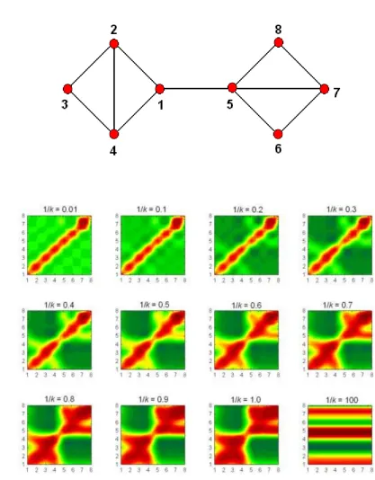
We start by considering a simple example which is illustrated in Fig. 1A. The logarithm of the transition matrix P for this graph has some negative out-diagonal entries, which indicates that some of its roots are not stochastic. We calculated 19 fractional powers of the transition matrix for this graph using the regularization method according to the algorithm of Charitos et al. [13]. In Fig. 1B we plot these matrices and fit the data points by using the weighted least square method [35] implemented in the STATISTICA package [36]. It can be clearly seen that the information diffuses from the main diagonal of the plots, in which it is concentrated at the starting of the process, to the regions outside the main diagonal. When the stationary state is reached the transition matrix has the form of the matrix , which when represented as in Fig. 1B has a shape characterized by multiple horizontal stripes; see the plot for 1 k/ 100.
12 Then, we calculated the same fractional powers without regularization by using the real Schur form [37], i.e., not necessarily stochastic roots. Using both approaches we calculate the mobility coefficient as defined by the expression (19). The mobility indices calculated by both approaches are quite close to each other, differing in less than 0.08% on average. We plotted the values of M versus k 1/k, observing that the mobility coefficient increases as a power law of the form
k c b
a Mk
/
1 , (11)
where 0.1121 with the regularization approach and 0.1111 without it. The correlation coefficient for the fitting is 0.9999 in both cases.
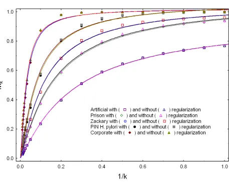
We further observe the universal character of this relation for random and real-world networks. Due to the practical importance of this result we investigate further the calculation of the mobility coefficient using both approaches for four real-world networks. The networks will be described below but for the time being we say that they have 34, 67, 710 and 1586 nodes. Their names are Zackary, Prison, PIN H. pylori and corporate (see below for description). In all cases the mobility indices obtained by the two methods were very close to each other, not differing in more than 1.3%. The mobility of the four networks obeys the relation (11) and the values of using the values of the mobility calculated by the two methods do not differ in more than 0.03 units. In Fig. 2 we plot the results obtained here for these networks with and without regularization.
13 Insert Fig. 2 about here.
B. Information mobility half-time
An important consequence of the existence of the relationship (11) is that we can obtain the value of the information mobility half-time, 1 k for which / 50 Mk 0.5. This is the time (in terms of 1/k) after which there will be more information transferred from the nodes than retained on them. We recall that at the beginning of the stochastic process all information is concentrated on the nodes with no mobility from one node to another. The value of 1 k is then given by / 50
d
c b a k
ln 5
. 0 ln exp /
1 50 . (12)
The value of 1 k for the artificial network illustrated in Fig. 1 is 0.288. This means / 50 that this network transfers 50% of the information through the nodes after approximately
3 /
1 of the time since the beginning of the stochastic process. In general, the smaller the value of 1 k the shorter the time used by the network to transfer 50% of the / 50 information through the nodes.
C. Information mobility in random networks
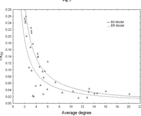
14 attachment mechanism for the BA model. We study random networks grown by these two mechanisms up to n = 1000 nodes, changing systematically the value of from 4 to 16. For every value of , we generated 1000 random networks. In Fig. 3 we illustrate a summary of the results obtained for the mobility indices calculated by using the expression (10).
Insert Fig. 3 about here.
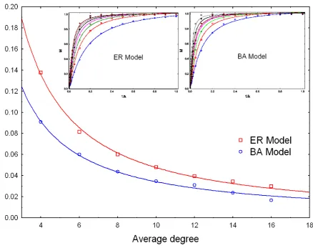
The first interesting result which is observed in Fig. 3 is that all ER and BA networks obey the power-law dependence (11) between the mobility and 1/k (see internal panels of Fig. 3). The second one is that 1 k decreases as a power-law with the / 50 increase of the average degree of the networks, 1/k50 ~ . The best fitted models are
1418 . 1 50 0.66137 /
1 k ER and 1/k50 BA 0.40297 1.0702. As can be seen in the main panel of Fig. 3 the decrease is fastest for the BA networks than for ER ones. For instance, for 16 the BA networks transfer 50% of the information at about 1/60 of the time after the initial step of the stochastic process. On the other hand, for similar ER network this percentage of transfer takes place at about 1/33 of the time after the initial step. The main conclusion here is that scale-free networks have better information mobility than random networks with a Poisson degree distribution. However, in the limit of very high average degree both kinds of networks tend to have the same information mobility (see the trend of the fitted curves in Fig. 3).
D. Information mobility in real-world networks
We study here 38 real-world complex networks accounting for ecological, biological, informational, technological and social systems. Description of all datasets and the appropriate references are given in Table 1.
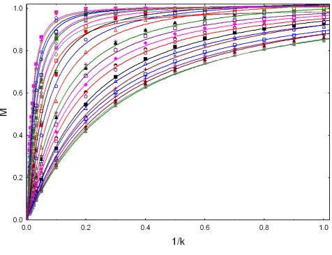
15 We start by generating the P matrices for all these networks. We then calculated the values of the mobility coefficient using the expression (10) and plot them versus 1/k in Fig. 4. As can be seen in this figure the mobility of all networks grows as a power-law function of 1/k. In all cases the power-law function is given by the expression (11) with coefficients ranging from 1.08 to 1.52.
Insert Fig. 4 about here.
The values of the power-law coefficients and those of 1 k reflect the large / 50 differences existing in the mobility of information for the networks studied (see Fig. 5). The network with the smallest 1 k is the Online Dictionary of Library and Information / 50 Science (ODLIS) in which 50% of the information is spread at 1/60 of the initial time of the stochastic process. A significant difference is observed for the networks with the largest values of 1 k , in which 50% of information is spread only after 1/3 of the / 50 initial time. In Fig. 5 we have included the plots of 1 k versus / 50 for ER and BA generated in the previous section. In general, most networks have information mobility which are better than ER random networks with the same average degree. For instance, only 12 out of 38 networks spread information at longer times than if they were random. On the other side of the coin, there are 12 out of 38 networks which spread information better than scale-free networks with the same average degree.
Insert Fig. 5 about here.
16 approach with the same average degree. A simple measure of this performance is given by the percentage of improvement in information mobility respect to the BA network,
BA k RW k
P % 100 50 / 50 , (13)
where RW stands for real-world networks. In Table 2 we give the values of the parameters calculated here for the 38 complex networks studied.
Insert Table 2 about here.
Let us consider the Online Dictionary of Library and Information Science (ODLIS) as an example. This network performs the spread of information P 180% better than the corresponding BA network. The Internet at the autonomous systems (AS) level as from April 1998 performs the spread of information P 490% better than the corresponding BA network. In general, the determination of what mechanism works behind this great performance of complex networks is still a puzzle. For instance, we know that these two networks are scale-free and display good expansion properties (super-homegeneity) [74-76], which can contribute to their higher performance but the airport transportation network in the US in 1997 does not have a power-law degree distribution and performs P 148% with respect to the BA model. The complexity of the performance of information mobility can be observed in the fact that the neural network of C. elegans, which also has exponential degree distribution and the average degree of 14 has only P 80% with respect to BA model. In summary, the mobility of 50% of information in a complex network appears to be related to several topological factors, such as the average degree, the degree distribution and the homogeneity of the network.
VI. SUMMARY
17 process taking place in the network in which information spread from the nodes. At the initial step all the information arising at a giving node stays there after certain number of steps. As the time progresses the information spreads from one node to another until a stationary state is reached at an infinite time. The transition matrix at unit time characterizing this process gives the probability that the information arising at a given node ends up at a target one. Then, the mobility of this information is introduced on the basis of the trace of the transition matrices at fractional time intervals. We have shown that the regularization method developed by Charitos et al. [13] is a suitable method of transforming the non-stochastic roots of the transition matrix into stochastic ones.
An interesting characteristic of complex networks is the fractional time at which they diffuse 50% of the information contained in its nodes (1 k ). The values of / 50 1 k / 50 increases with the average degree in random networks with a Poisson or a power-law degree distribution. Scale-free networks display better spread of information than the random networks with a Poisson degree distribution. The mobility coefficient displays a universal power-law relationship with the fractional time for all random and real-world networks.
We have analyzed all the new concepts by studying 38 real-world networks. We find that some real-world networks perform information spreading even better than scale-free networks with the same average degree. The network versions of the Internet at the AS level analyzed here display the best performance in information spreading among all the networks studied.
ACKNOWLEDGEMENTS
18 in this work and reviewing a former version of the manuscript. N. Hatano is thanked for a careful revision of this work. This work is partially supported by the Principal of the University of Strathclyde through the New Professor’s Fund. Critics and comments of two annonomous referees contributed to a significant improvement of the presentation of this work.
19 APPENDIX.
ON FRACTIONAL POWERS OF THE TRANSITION MATRIX P
There are two important questions in relation to the roots of the stochastic matrix P. The first is about the existence of such roots and the second is about their
stochasticity. To answer the first, let us define a diagonal matrix S diag1TeA 1 , where 1 is a n 1 all-ones vector. Then, the row-stochastic matrix of P can be written as
A
S
P e . Now, the question about the existence of the transition matrix of the Markov chain is transformed into the question about the existence of the kth root of A
S P e . It is easy to show that the transition matrix A
S
P e has no eigenvalues on and consequently it has a principal kth root X P1/k for any k. However, the existence of the principal kth root does not guaranty that such roots are stochastic. Thus, we need to analyze the second question posted below.
The analysis of the stochasticity of the roots of the transition matrix is a well known ill-posed problem [16]. Unfortunately, when dealing with real-world complex networks none of the previous analytical results [14] for the stochasticity of the transition matrices are fulfilled. Consequently we have to deal with the stochasticity of the roots of the transition matrix of general complex networks in a case-by-case basis.
20 215 . 0 210 . 0 183 . 0 210 . 0 183 . 0 150 . 0 237 . 0 216 . 0 180 . 0 216 . 0 123 . 0 203 . 0 245 . 0 203 . 0 225 . 0 150 . 0 180 . 0 216 . 0 237 . 0 216 . 0 123 . 0 203 . 0 225 . 0 203 . 0 245 . 0 P 440 . 2 175 . 1 045 . 0 175 . 1 045 . 0 844 . 0 892 . 2 037 . 1 037 . 1 031 . 0 973 . 0 954 . 2 973 . 0 977 . 0 8435 . 0 037 . 1 892 . 2 037 . 1 0301 . 0 973 . 0 977 . 0 973 . 0 954 . 2 ln 0.025 0.025 P
The first root of the transition matrix of this graph which is not stochastic is the 61th. This indicates that the process can be considered as a Markov chain for all fractional time between 1/60 and the unit time. As we have stated before the non-stochastic root matrices can be slightly perturbed to stochastic ones. Here we apply Charitos et al.’s [13]
algorithm of regularization for transforming the roots of the matrix P into stochastic ones by using perturbations. The algorithm is described below.
Let 1/k P
X . The algorithm proposed by Charitos et al. [13] searches a transition matrix X* from the set of all n ntransition matrices that, when raised to the power k, most closely matches the transition matrix P. That is,
X A X* argmin ˆ
A ,
where is a suitable norm in the space of n n matrices and Xˆ is the matrix resulting from removing the imaginary part of all the entries of X. The algorithm calculates *
X
on a row-by-row basis for each row of Xˆ by searching a vector
i i p Simml
21 where lp is a vector norm measuring the distance between two points in the n-dimensional space and Simim is an n-dimensional simplex. The algorithm to obtain * as taken from Charitos et al. [13] is,
1. If ˆij 0, j 1,,n, then STOP; i* aˆi. Otherwise 2. Compute the quantity :ˆ 0 ˆ
ij a
j aij and the number of positive entries 0
ˆ # jaij
m .
3a. If aˆij 0, then set aˆij 0, j 1,,n.
3b. If aˆij 0, then set aˆij aˆij /m, j 1,,n. 4. Go to step 1.
We use here a Matlab code gently provided by T. Charitos to make the calculation of the stochastic roots of the transition matrix P. Note that the code by Charitos et al. [13] provides the consolidated algorithm as proposed in the paper that combines the previous 4-step procedure for the Lp-norm with two subalgorithms that use the relative entropy measure for each row to produce the optimal short interval transition matrix. In addition, the code includes the 'entry fix' as proposed by Charitos et al. [13] for avoiding cases where a short interval transition matrix has a zero in an entry where the corresponding entry in the original transition matrix is positive. For instance, in the example given below we calculate the 61th root of the transition matrix P,
9610 . 0 0184 . 0 0010 . 0 0184 . 0 0010 . 0 0132 . 0 9541 . 0 0163 . 0 0163 . 0 0007 . 0 0153 . 0 9531 . 0 0153 . 0 0155 . 0 0132 . 0 0163 . 0 9541 . 0 0163 . 0 0007 . 0 0153 . 0 0155 . 0 0153 . 0 9531 . 0 61 / 1 6 6 10 6.44 10 6.44 P
22 code can be obtained at The Matrix Function Toolbox (www.maths.manchester.ac.uk/~higham/mftoolbox). However, when we applied the algorithm of Charitos et al. [13] we obtain the following stochastic matrix, which is very close to the previous one:
9610 . 0 0184 . 0 0010 . 0 0184 . 0 0010 . 0 0132 . 0 9513 . 0 0163 . 0 0029 . 0 0163 . 0 0007 . 0 0153 . 0 9531 . 0 0153 . 0 0155 . 0 0132 . 0 0029 . 0 0163 . 0 9513 . 0 0163 . 0 0007 . 0 0153 . 0 0155 . 0 0153 . 0 9531 . 0 61 / 1 P
When we analyze the roots of the transition matrix P, we are only considering some time intervals of the stochastic process. For instance, if we consider P1/2 we obtain the transition matrix for a period of time which is only one half of the unit time. Then, in order to investigate what happens at time steps closer to the unit time we need to know
1 k
T (considering that k T
P ). One strategy that we consider here is to find the t th root of P and then rising P1/t to the power p t 1: Pt 1/t Tt 1k/t TkT k/t. Then, for sufficiently large values of t we have
1 /
/ 1
lim
lim k k t k
k t t t
23 [1] S. M. Lipset and R, Bendix, Social Mobility in Industrial Society, (Transaction
Publications, 1991).
[2] B. R. Schiller, Am. Econ. Rev. 67, 926 (1977). [3] A. F. Shorrocks, Ecocomica 50, 3 (1983).
[4] S. S. Kuznets, Modern Economic Growth: Rate, Structure and Spread (Yale University Press, New Haven, 1966).
[5] N. Ding, N. Xi and Y. Wang, Physica A 367, 415 (2006).
[6] J. Geweke, R. C. Marshall and G. A Zarkin, Econometrica 54, 1407 (1986). [7] A. F. Shorrocks, Econometrica 46, 1013 (1978).
[8] U. Cantner and J. J. Krüger, Rev. Ind. Org. 24, 267 (2004).
[9] F. V. Waugh and M. E. Abel, J. Amer. Statist. Assoc. 62, 1018 (1967). [10] R. B. Israel, J. S. Rosenthal and J. Z. Wei, Math. Finan. 11, 245 (2001). [11] R. A. Jarrow, D. Lando and S. M. Turnbull, Rev. Finan. Stud. 10, 481 (1997). [12] Q.-M. He and E. Gunn, J. Syst. Sci. Syst. Eng. 12, 210 (2003).
[13] T. Charitos, P. R. de Waal and L. C. van der Gaag, Statist. Med. 27, 905 (2008). [14] N. J. Higham and L. Lin, On pth roots of stochastic matrices.
http://eprints.ma.man.ac.uk/1241/01/covered/MIMS_ep2009_21.pdf [15] B. Singer and S. Spilerman, Am. J. Sociol. 82, 1 (1976).
[16] A. Kreinin and M. Sidelnikova, Algor. Res. Quat. 4, 23 (2001).
[17] N. L. Biggs, Algebraic Graph Theory (Cambridge University Press, Cambridge, England, 1993).
[18] N. J. Higham, Function of Matrices. Theory and Computation (SIAM, Philadelphia, 2008).
24 [20] E. Estrada and N. Hatano, Phys. Rev. E. 77, 036111 (2008).
[21] T. D slić, Chem. Phys. Lett. 412, 336 (2005). [22] E. Estrada, Proteomics 6, 35 (2006).
[23] A. Platzer, P. Perco, A. Lukas and B. Mayer, BMC Bioinformatics 8, 224 (2007). [24] E. Zotenko, J. Mestre. D. P. O’Leary and T. M. Przytycka, PLOS. Computational
Biology 4, 1 (2008).
[25] M. Jungsbluth, B. Burghardt and A. K. Hartmann, Physica A 381, 444 (2007). [26] V. V. Kerrenbroeck and E. Marinari, Phys. Rev. Lett. 101, 098701 (2008). [27] L. Da Fontoura Costa, M. A. Rodrigues Tognetti, F. Physica A 387, 6201 (2008). [28] D. H. Higham and J. Croft, J. Royal Soc., Interface, in print.
[29] J. A. de la Peña, I. Gutman and J. Rada, Lin. Algebra Appl. 427, 70 (2007). [30] I. Gutman and A. Graovac, Chem. Phys. Lett. 436, 294 (2007).
[31] Y. Ginosar, I. Gutman, T. Mansour and M. Schork, Chem. Phys. Lett. 454, 145 (2008).
[32] R. Carbó-Dorca, J. Math. Chem. 44, 373 (2008).
[33] M. Robbiano, R. Jimenez and L. Medina, MATCH: Comm. Math. Comput. Chem. 61, 369 (2009).
[34] R. Norris, Markov Chains (Cambridge University Press, Cambridge, England, 1997)
[35] D.H. McLain, Comput. J. 17, 318 (1974). [36] STATISTICA 6.0., StatSoft Inc., 2002.
[37] D. A. Bini, N. J. Higham and B. Meini, Lin. Alg. Appl. 39, 349 (2005). [38] P. Erd s and A. Rényi, Public. Math. 6, 290 (1959).
25 [40] Roget´s Thesaurus of English Words and Phrases (2002). Project Gutenberg.
http://gutenberg.net/etext/22
[41] ODLIS: Online Dictionary of Library and Information Science (2002).
http://vax.wcsu.edu/library/odlis.html
[42] B. Jones, Computational Geometry Database, February, 2002.
http://compgeom.cs.edu/~jeffe/compgeom/biblios.html.
[43] G. F. Davis, M. Yoo and W.E. Baker, Strateg. Organ. 1, 301 (2003).
[44] Data for this project was provided in part by NIH grants DA12831 and HD41877, those interested in obtaining a copy of these data should contact James Moody
[45] W. Zachary, J. Anthropol. Res. 33, 452 (1977). [46] L. D. Zeleny, Sociometry 13, 314 (1950).
[47] http://vlado.fmf.uni-lj.si/pub/networks/data/Ucinet/UciData.htm
[48] J. J. Potterat, L. Philips-Plummer, S. Q. Muth, R. B. Rothenberg, D. E. Woodhouse, T. S. Maldonado-Long, H. P. Zimmerman and J. B. Muth, Sex. Transm. Infect. 78, i159 (2002).
[49] P. G. Lind, M. C. González, and H. J. Herrmann, Phys. Rev. E 72, 056127 (2005).
[50] V. Batagelj, A. Mrvar, Graph Drawing Contest 2001. http://vlado.fmf.uni-lj.si/pub/GD/GD01.htm
[51] N. P. Hummon, P. Doreian, L. C. Freeman, Know.-Creat. Diffus. Util. 11, 459, (1990).
26 [53] Taken from http://vlado.fmf.uni-lj.si/pub/networks/data/default.htm as collected from the Garfield’s collection of citation network datasets (http://www.garfield.library.upenn.edu/histcomp/index.html).
[54] Taken from http://vlado.fmf.uni-lj.si/pub/networks/data/default.htm as collected from North American Transportation Atlas Data (NORTAD):
http://www.bts.gov/publications/north_american_transportation_atlas_data/
[55] M. Faloutsos, P. Faloutsos, C. Faloutsos, Comp. Comm. Rev. 29, 251 (1999). [56] COSIN database: http://www.cosin.org.
[57] R. Milo, S. Itzkovitz, N. Kashtan, R. Levitt, S. Shen-Orr, I. Ayzenshtat, M. Sheffer, U. Alon, Science 303, 1538 (2004).
[58] D. Bu, Y. Zhao, L. Cai, H. Xue, X. Zhu, H. Lu, J. Zhang, S. Sun, L. Ling, N. Zhang, G. Li, R. Chen, Nucl. Acids Res. 31, 2443 (2003).
[59] J.-C. Rain, et al., Nature 409, 211 (2001).
[60] M.-F. Noirot-Gros, E. Dervyn, L. J. Wu, P. Mervelet, J. Errington, S. D. Ehrlich and P. Noirot, Proc. Natl. Acad. Sci. USA 99, 8342 (2002).
[61] M. Motz, I. Kober, C. Girardot, E. Loeser, U. Bauer, M. Albers, G. Moeckel, E. Minch, H. Voss, C. Kilger and M. Koegl, J. Biol. Chem. 277, 16179 (2002). [62] D. J. LaCount, et al., Nature 438, 103 (2005).
[63] J.-F. Rual, et al., Nature 437, 1173 (2005).
[64] S. Shen-Orr, R. Milo, S. Mangan, U. Alon, Nature Genet. 31, 64 (2002).
[65] R. Milo, S. Shen-Orr, S. Itzkovitz, N. Kashtan, D. Chklovskii, U. Alon, Science 298, 824 (2002).
27 [67] N. D. Martinez, B. A. Hawkins, H. A. Dawah, B. P. Feifarek, Ecology 80, 1044
(1999).
[68] J. Memmott, N. D. Martinez, J. E. Cohen, J. Anim. Ecol. 69, 1 (2000).
[69] C. Townsend, R. M. Thompson, A. R. McIntosh, C. Kilroy, E. Edwards, M. R. Scarsbrook, Ecol. Lett. 1, 200 (1998).
[70] R. R. Christian, J. J. Luczkovich, Ecol. Mod. 117, 99 (1999). [71] P. H. Warren, Oikos 55, 299 (1989).
[72] P. Yodzis, Ecology 81, 261 (2000).
[73] S. Opitz, ICLARM Tech. Rep. 43, Manila, Philippines (1996). [74] E. Estrada, Europhys. Lett. 73, 649 (2006).
28 Table 1. Brief description of the real-world complex networks studied.
Name Nodes Links Description Ref.
Roget 994 3640 Vocabulary network of words related by their definitions in Roget’s Thesaurus of English. Two words are connected if one is used in the definition of the other.
40
ODLIS 2898 16376 Vocabulary network of words related by their definitions in the Online Dictionary of Library and Information Science. Two words are connected if one is used in the definition of the other.
41
Geom 3621 9461 Collaboration network of scientists in the field of computational geometry.
42
Corporate 1586 11540 Network of the American corporate elite formed by the directors of the 625 largest corporations that reported the compositions of their boards selected from the Fortune 1000 in 1999.
43
Prison 67 142 Social network of inmates in prison who chose “What fellows on the tier are you closest friends with?”
44
Zachary 34 78 Social network of friendship between members of the Zachary karate club.
45
College 32 96 Social network among college students in a course about leadership. The students choose which three members they wanted to have in a committee.
46
Galesburg 31 67 Friendship ties among 31 physicians. 47
High Tech 33 91 Friendship ties among the employees in a small hi-tech computer firm which sells, installs, and maintains computer systems.
47
29 during its early epidemic phase in Colorado Springs, USA (sexual and injecting drugs partners) from 1985-1999.
Heterosexual 82 83 Heterosexual contacts which were extracted at the Cadham Provincial Laboratory and is a 6-month block data between November 1997 and May 1998.
49
Homosexual 250 266 Contact tracing study, from 1985 to 1999, for HIV tests in Colorado Springs, USA, where most of the registered contacts were homosexual.
49
GD 249 635 Citation network of papers published in the Proceedings of Graph Drawing during the period 1994-2000.
50
Centrality 118 613 Citation network of papers published in the field of network centrality.
51,52
Small World 233 994 Citation network of papers that cite S. Milgram's 1967 Psychology Today paper or use Small World in the title.
53
USAir97 332 2126 Airport transportation network between airports in US in 1997.
54 Int_1997 Int_1998 3015 3522 5156 6324
The internet at the autonomous system (AS) level as of September 1997 and of April 1998 taken from the COSIN database.
55,56 Electronic1 Electronic2 Electronic3 122 252 512 189 399 819
Electronic sequential logic circuits parsed from the ISCAS89 benchmark set, where nodes represent logic gates and flip-flops.
57 PIN1 PIN2 PIN3 2224 710 84 6608 1396 98
Protein-protein interaction networks in S. cereviciae, H. pylori, B. subtilis, A. fulgidus, P. falciparum and H. sapiens.
30 PIN4
PIN5 PIN6
32 229 2783
36 604 6007
Trans-Ecoli 328 456 Direct transcriptional regulation between operons in Escherichia coli.
57,64
Trans-yeast 662 1062 Direct transcriptional regulation between genes in Saccaromyces cerevisae.
57,65
Neurons 280 1973 Neuronal synaptic network of the nematode C. elegans, which includes all data except muscle cells and using all synaptic connections.
57,66
Grassland 75 113 All vascular plants and all insects and trophic interactions found inside stems of plants collected from 24 sites distributed within England and Wales.
67
Scotch Broom 154 366 Trophic interactions between the herbivores, parasitoids, predators and pathogens associated with broom, Cytisus scoparius, collected in Silwood Park, Berkshire, England, UK.
68
Canton Creek 108 707 Primarily invertebrates and algae in a tributary, surrounded by pasture, of the Taieri River in the South Island of New Zealand.
69
Chesapeake Bay
33 71 The pelagic portion of an eastern U.S. estuary, with an emphasis on larger fishes.
70
Coachella Valley
30 241 Wide range of highly aggregated taxa from the Coachella Valley desert in southern California.
71
Benguela 29 191 Marine ecosystem of Benguela off the southwest coast of South Africa.
72
Reef Small 50 503 Caribbean coral reef ecosystem from the Puerto Rico-Virgin Island shelf complex.
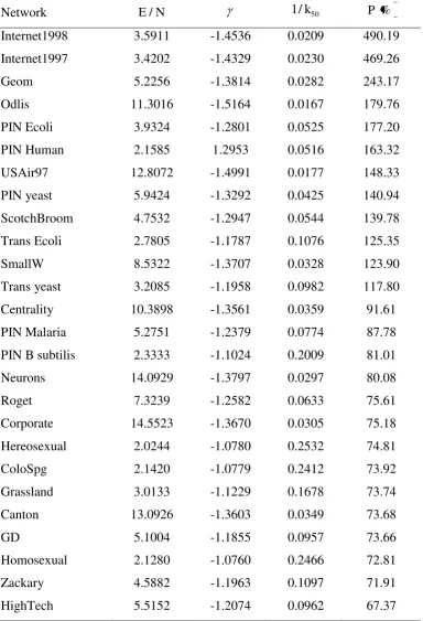
31 Table 2. The densities (E /N), the power-law coefficients ( ), the half-times (1 k ) / 50 and the performance (P % ) (see text for definitions) for the 38 real-world complex networks studied here. The networks are ranked in decreasing order of their performances.
Network E /N 1 k / 50 P %
Internet1998 3.5911 -1.4536 0.0209 490.19
Internet1997 3.4202 -1.4329 0.0230 469.26
Geom 5.2256 -1.3814 0.0282 243.17
Odlis 11.3016 -1.5164 0.0167 179.76
PIN Ecoli 3.9324 -1.2801 0.0525 177.20
PIN Human 2.1585 1.2953 0.0516 163.32
USAir97 12.8072 -1.4991 0.0177 148.33
PIN yeast 5.9424 -1.3292 0.0425 140.94
ScotchBroom 4.7532 -1.2947 0.0544 139.78
Trans Ecoli 2.7805 -1.1787 0.1076 125.35
SmallW 8.5322 -1.3707 0.0328 123.90
Trans yeast 3.2085 -1.1958 0.0982 117.80
Centrality 10.3898 -1.3561 0.0359 91.61
PIN Malaria 5.2751 -1.2379 0.0774 87.78
PIN B subtilis 2.3333 -1.1024 0.2009 81.01
Neurons 14.0929 -1.3797 0.0297 80.08
Roget 7.3239 -1.2582 0.0633 75.61
Corporate 14.5523 -1.3670 0.0305 75.18
Hereosexual 2.0244 -1.0780 0.2532 74.81
ColoSpg 2.1420 -1.0779 0.2412 73.92
Grassland 3.0133 -1.1229 0.1678 73.74
Canton 13.0926 -1.3603 0.0349 73.68
GD 5.1004 -1.1855 0.0957 73.66
Homosexual 2.1280 -1.0760 0.2466 72.81
Zackary 4.5882 -1.1963 0.1097 71.91
[image:31.595.85.470.203.767.2]32
PIN A fulgidus 2.2500 -1.0777 0.2601 65.06
Chesapeake 4.3030 -1.1503 0.1389 60.85
SawMill 3.4444 -1.1102 0.1782 60.20
Galesburg 4.3226 -1.1452 0.1408 59.75
ReefSmall 20.1200 -1.3999 0.0279 58.14
Benguela 13.1724 -1.3364 0.0442 57.71
Prison 4.2388 -1.1293 0.1490 57.64
Coachella 16.0667 -1.3637 0.0364 56.66
Electronic3 3.1992 -1.0876 0.2110 55.01
Electronic2 3.1667 -1.0853 0.2169 54.11
Electronic1 3.0984 -1.0822 0.2259 53.19
33 Figure captions
Fig. 1. (color online) An artificial network (A) used to illustrate the process of information mobility (B) for different values of fractional times 1 k/ 1. The transition matrix for the value 1 k/ 100 is also illustrated as a representation of the stationary state.
Fig. 2. (color online) Illustration of the results obtained by calculating the fractional powers of the transition matrix with and without regularization for the artificial network illustrated in Fig. 1 and for four real-world networks.
Fig. 3. (color online) (Inner panels) Illustration of the power-law dependence between the information mobility and the fractional time for random networks with Poisson and scale-free degree distributions. It is seen that as the time progresses the mobility grows until reaching a saturation at values about 1 k/ 1. (Main panel) Relation between the information mobility half-time and the average degree for the random networks generated by ER and BA models. It is observed that as the average degree increases the mobility half-time goes to zero following a power-law decay. For small average degree it is seen that scale-free networks (BA) display larger mobility half-time than ER networks. Fig. 4. (color online) Illustration of the power-law dependence of the information mobility on the fractional time for 38 real-world networks. It is seen that as the time progresses from zero to one the information mobility grows following a power-law. At infinite times a value of M 1 is obtained.
34 Fig. 1.
A