Securing location discovery in wireless sensor networks

Rochester Institute of Technology

RIT Scholar Works

Theses Thesis/Dissertation Collections

2009

Securing location discovery in wireless sensor

networks

Wisam F. Kadhim

Follow this and additional works at:http://scholarworks.rit.edu/theses

This Thesis is brought to you for free and open access by the Thesis/Dissertation Collections at RIT Scholar Works. It has been accepted for inclusion Recommended Citation

Securing Location Discovery

in Wireless Sensor Networks

by

Wisam F. Kadhim

A Thesis Submitted in Partial Fulfillment of the Requirements for the Degree of Master of Science in Computer Science

Supervised by Dr. Minseok Kwon Department of Computer Science

Golisano College of Computing and Information Sciences Rochester Institute of Technology

Rochester, NY August 2009

Approved By:

_____________________________________________ ___________ ___ Dr. Minseok Kwon

Advisor – R.I.T. Dept. of Computer Science

_ __ ___________________________________ ___ _________ _____ Dr. Zack Butler

Reader – R.I.T. Dept. of Computer Science

_____________________________________________ ______________ Dr. Hans-Peter Bischof

Thesis Release Permission Form

Rochester Institute of Technology

Golisano College of Computing and Information Sciences

Title: Securing Location Discovery in Wireless Sensor Networks

I, Wisam F. Kadhim, hereby grant permission to the Wallace Memorial Library to reproduce my thesis in whole or part.

_________________________________ Wisam F. Kadhim

iii

Dedication

To my family…

Acknowledgements

So many people have influenced who I am today and have helped guide me to this point.

The following is only a small subset of those who deserve my heartfelt thanks. My

thanks to Professor Kwon for his unwavering guidance during my work. Also, to

Professor Bischof for all the extraordinary support he has given me. To Professor Steele

and Professor Schreiner, for encouraging new ways of thinking and indirectly pushing me

to explore my artistic side, and to Professor Butler for reviewing this work. I also thank

Jaime Burns and Ara Murad for graciously editing several drafts and pushing me towards

v

Abstract

Providing security for wireless sensor networks in hostile environments has a significant importance. Resilience against malicious attacks during the process of location discovery has an increasing need. There are many applications that rely on sensor nodes' locations to be accurate in order to function correctly. The need to provide secure, attack resistant location discovery schemes has become a challenging research topic. In this thesis, location discovery techniques are discussed and the security threats and attacks are explained. I also present current secure location discovery schemes which are developed for range-based location discovery.

Table of Contents

Chapter 1: INTRODUCTION 1

1.1 Classification of Localization Techniques 2

1.2 Security Threats Associated with Location Discovery 4

Chapter 2: EXISTING SECURE LOCATION DISCOVERY SCHEMES 6

2.1 Statistical Based Location Discovery Scheme 7

2.2 Voting Based Scheme 10

Chapter 3: PROPOSED SECURE LOCATION DISCOVERY SCHEMES 13

3.1 Enhanced Voting Based Scheme 13

3.2 Secure Range-Free Location Discovery Scheme 16

Chapter 4: IMPLEMENTATION AND TEST RESULTS 25

4.1 Implementation on Sun SPOTs and System Architecture 25

4.2 Test Cases and Simulation Results 28

CONCLUSION 38

vii

List of Figures

1.1 Attack patterns against location discovery schemes 4

2.1 The voting based location estimation 11

3.1 Enhanced voting based scheme 14

3.2 Overlapping of candidate rings and a cell 15

3.3 APIT location discovery scheme 17

3.4 Triangle creation method 19

3.5 Barycentric coordinates 20

3.6 Point in triangle test 21

3.7 Proposed secure range-free location discovery scheme 23

4.1 Sun SPOT sensor 26

4.2 System architecture block diagram 27

4.3 Block diagram of emulator architecture in Solarium 29

4.4 Sun SPOTs experiment snapshot 30

4.5 Sun SPOTs experiment layout map and results 31

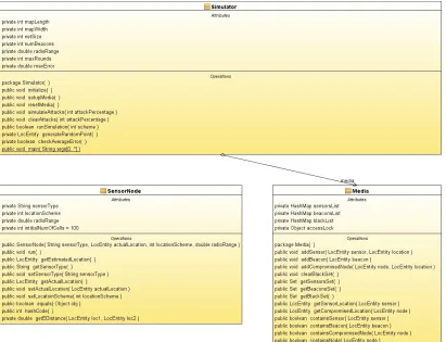
4.6 Simulator class diagram 32

4.7 Security resilience simulation test results 35

4.8 Location discovery execution time 36

List of Tables

4.1 Sun SPOTs experiment results 31

ix

Glossary

AoA Angle of Arrival

APIT Area based Point In Triangulation

BARMMSE Brute-force Attack Resistant Minimum Mean Square Error CLDC Connected Limited Device Configuration

CoG Center of Gravity

EARMMSE Enhanced greedy Attack Resistant Minimum Mean Square Error GARMMSE Greedy Attack Resistant Minimum Mean Square Error

GPS Global Positioning System GUI Graphical User Interface LED Light Emitting Diode

MIDP Mobile Information Device Profile MMSE Minimum Mean Square Error

OS Operating System PIT Point in Triangulation

RADAR An In-Building RF-based User Location and Tracking System RGB Red/Green/Blue

ROPE Rubust Position Estimation RSSI Received Signal Strength Indicator SeRLoc Secure Range independent Localization

SPINE Secure Positioning In sensor Networks SPOT Small Programmable Object Technology TDoA Time Difference of Arrival

ToA Time of Arrival VM Virtual Machine

Chapter 1

I

Wireless Sensor Networks (WSN) are networks made of small, battery-powered, memory-constrained devices called sensor nodes, which have the capability of wireless communication over a restricted area. Due to memory and power constraints, they need to be well-arranged to build a fully functional network. Wireless sensors' locations are vital to many sensor network applications such as environmental monitoring, military applications, and many other applications which require sensors' location information to fulfill their tasks. There are also several fundamental techniques [8] developed for wireless sensor networks which require wireless sensor nodes' locations, for instance geographic routing protocols where sensor nodes make routing decisions based on their own location as well as their neighbors' locations.

Despite recent advances, location discovery for wireless sensor networks in hostile environments has been typically overlooked. Most of the existing location discovery protocols are vulnerable in the presence of malicious attacks. An attacker may provide incorrect location references by replaying the beacon packets intercepted in different locations. Furthermore, an attacker may compromise a beacon node and distribute malicious location references by lying about the beacon node’s location or manipulating the beacon signals. In either of these cases, non-beacon nodes will determine their locations incorrectly. The security of location discovery can certainly be enhanced by authentication. However, authentication does not guarantee the security of location discovery. An attacker may forge beacon packets with keys learned through compromised nodes, or replay beacon signals intercepted in different locations [8].

Several attack-resistant location estimation techniques were developed to tolerate the malicious attacks against range-based location discovery in wireless sensor networks. This thesis focuses on the voting-based location estimation technique developed in [8, 9], where the deployment field is quantized into a grid of cells and has each location reference vote on the cells in which the node may reside with iterative refinement of the voting results so that it can be executed in resource constrained sensor nodes.

2

location discovery scheme. This would provide a less complicated, cost-effective, and more applicable solution for wireless sensor networks.

1.1

Classification of Localization Techniques

1.1.1 Direct approaches

This is also known as absolute localization. The direct approach itself can be classified into two types: Manual configuration and GPS-based localization. The manual configuration method is very cumbersome and expensive. It is neither practical nor scalable for large scale WSNs and in particular, does not adapt well for WSNs with node mobility. On the other hand, in the GPS-based localization method, each sensor is equipped with a GPS receiver. This method adapts well for WSNs with node mobility.

However, there is a downside to this method. It is not economically feasible to equip each sensor with a GPS receiver since WSNs are deployed with hundreds of thousands of sensors. This increases the size of each sensor, rendering them unfit for pervasive environments. Also, the GPS receivers only work well outdoors on earth and have line-of-sight requirement constraints. Such WSNs cannot be used for underwater applications like habitat monitoring, water pollution level monitoring, and tsunami monitoring [1].

1.1.2 Indirect approaches

The indirect approach of localization is also known as relative localization since nodes position themselves relative to other nodes in their vicinity. The indirect approaches of localization were introduced to overcome some of the drawbacks of the GPS-based direct localization techniques while retaining some of their advantages, like accuracy of localization. In this approach, a small subset of nodes in the network, called the beacon nodes, are either equipped with GPS receivers to compute their location or are manually configured with their location. These beacon nodes then send beams of signals providing their location to all sensor nodes in their vicinity that do not have a GPS receiver. Using the transmitted signal containing the location information, sensor nodes compute their location. This approach effectively reduces the overhead introduced by the GPS-based method [1].

Within the indirect approach, the localization process can be classified into the following two categories:

Range-based:

In range-based localization, the location of a node is computed relative to other nodes in its vicinity. Range-based localization depends on the assumption that the absolute distance between a sender and a receiver can be estimated by one or more features of the communication signal from the sender to the receiver. The accuracy of such estimation, however, is subject to the transmission medium and surrounding environment. Range based techniques usually rely on complex hardware which is not feasible for WSNs since sensor nodes are highly resource-constrained and have to be produced at throw-away prices as they are deployed in large numbers. The features of the communication signal that are frequently used in literature for range-based localization are as follows:

• Angle of Arrival (AoA): Range information is obtained by estimating and mapping relative angles between neighbors.

• Received Signal Strength Indicator (RSSI): Use a theoretical or empirical model to translate signal strength into distance. RADAR [1, 11] is one of the first to make use of RSSI.

• Time of Arrival (ToA): To obtain range information using ToA, the signal propagation time from source to destination is measured. A GPS is the most basic example that uses ToA. To use ToA for range estimation, a system needs to be synchronous, which necessitates the use of expensive hardware for precise clock synchronization with the satellite.

• Time Difference of Arrival (TDoA): To obtain the range information using TDoA, an ultrasound is used to estimate the distance between the node and the source. Like ToA, TDoA necessitates the use of special hardware, rendering it too expensive for WSNs.

Range-free:

1.2

Security Threats Associated with Location Discovery

In hostile environments, an

via injecting misleading location references. The attacker can either be an insider or an outsider. As an insider, the attacker has access to all of the cryptographic keyi

held by a node. This is potentially dangerous since the attacker can now claim to be a legitimate part of the network. Authentication or verification via password and other mechanisms give up under this attack model. On the other hand, in the o

model, the attacker is outside the network and has no information about cryptographic keys and passwords necessary for authentication. The attacker can only capture a node but cannot extract the sensitive information. This model is comparati

detrimental, but harmful nonetheless. So, for localization process to be secured it has to be robust in its defense against both outsider and insider attacks [1].

Figure 1.1: Attack patterns against location discovery schemes [1, 8].

Some attacks that have been discussed for nearly a decade in literature that are the most common against localization schemes are as follows:

• Masquerading and Compromising Beacon Nodes:

attacker would impersonate a beacon node and send misleadi

its location to divert the other benign nodes from discovering their accurate location, as shown in

nodes through physical capture, and use the compromised beacon nodes to inject

4

Security Threats Associated with Location Discovery

In hostile environments, an adversary can compromise sensor nodes location discovery via injecting misleading location references. The attacker can either be an insider or an outsider. As an insider, the attacker has access to all of the cryptographic keyi

held by a node. This is potentially dangerous since the attacker can now claim to be a legitimate part of the network. Authentication or verification via password and other under this attack model. On the other hand, in the outsider attack model, the attacker is outside the network and has no information about cryptographic keys and passwords necessary for authentication. The attacker can only capture a node but cannot extract the sensitive information. This model is comparati

detrimental, but harmful nonetheless. So, for localization process to be secured it has to be robust in its defense against both outsider and insider attacks [1].

Attack patterns against location discovery schemes [1, 8].

cks that have been discussed for nearly a decade in literature that are the most common against localization schemes are as follows:

Masquerading and Compromising Beacon Nodes: In masquerading, the

attacker would impersonate a beacon node and send misleading information about its location to divert the other benign nodes from discovering their accurate location, as shown in Figure 1.1(a). An attacker can also compromise beacon nodes through physical capture, and use the compromised beacon nodes to inject

can compromise sensor nodes location discovery via injecting misleading location references. The attacker can either be an insider or an outsider. As an insider, the attacker has access to all of the cryptographic keying material held by a node. This is potentially dangerous since the attacker can now claim to be a legitimate part of the network. Authentication or verification via password and other utsider attack model, the attacker is outside the network and has no information about cryptographic keys and passwords necessary for authentication. The attacker can only capture a node but cannot extract the sensitive information. This model is comparatively less detrimental, but harmful nonetheless. So, for localization process to be secured it has to

Attack patterns against location discovery schemes [1, 8].

cks that have been discussed for nearly a decade in literature that are the

In masquerading, the

ng information about its location to divert the other benign nodes from discovering their accurate

misleading location references that would affect location discovery for other benign nodes, as shown in Figure 1.1(b) [8].

• Replay Attack: A replay attack is the easiest and most commonly used by

attackers. Specifically, when an attacker’s capability is limited, i.e., the attacker cannot compromise more than 1 node; this is the most preferred attack. In a replay attack, the attacker merely jams the transmission between a sender and a receiver and later replays the same message, posing as the sender. The other way to launch a replay attack is, as shown in Figure 1.1(c). A replay attack has a two-fold

consequence. First, the attacker is replaying the message of another node. Second, the attacker is transmitting stale information. In particular, the chances of the information being stale are higher in networks with higher node mobility. When replay attacks are launched on the localization process, a localizing node will receive an incorrect reference thereby localizing incorrectly. Unlike a wormhole attack, a single node can disrupt the network with a replay attack [1, 8].

• Sybil Attack: The Sybil attack requires a more sophisticated attacker compared

to the replay attack. In a Sybil attack, a node claims multiple identities in the network. When launched on localization, localizing nodes can receive multiple location references from a single node leading to incorrect location estimation. Like the replay attack, the Sybil attack can also be launched by a single node since there is no need for collusion among nodes to launch this attack [1].

• Wormhole Attack: A wormhole attack is the most complicated of all the

6

Chapter 2

E

S

L

D

S

Several techniques have been developed to deal with the security problems of location discovery in wireless sensor networks. The location verification technique proposed in Secure Verification of Location Claims [14] can be used to verify the relative distance between a verifying node and a sensor node. However, it does not provide a solution to conduct secure location estimation at non-beacon nodes. A robust location detection is developed in Robust Location Detection [13] using the idea of majority voting, but it cannot be directly applied in resource constrained sensor networks due to its high computation and storage overheads. A robust statistical method is independently discovered in Robust Statistical Method [7] to achieve robustness through Least Median of Squares.

SeRLoc [5] protects location discovery with the help of sectored antennae at beacon nodes. Similar to the voting-based scheme, SeRLoc can tolerate malicious attacks by adopting the idea of majority voting. SPINE [2] was developed to protect location discovery by using verifiable multi-lateration. However, the distance bounding techniques required for verifiable multi-lateration may not be available in sensor networks due to the difficulties in dealing with the external attacks in ultrasound-based distance bounding and achieving nanosecond processing and time measurements in radio-based distance bounding. ROPE [6] is developed by integrating SeRLoc and SPINE. However, it still requires nanosecond processing and time measurements that are not desirable for the current generation of sensor networks.

2.1

Statistical Based Location Discovery Scheme:

Intuitively, a location reference introduced by a malicious attack is aimed at misleading a sensor node about its location. Thus, it is usually different from benign location references. When there are redundant location references, there must be some inconsistency between the malicious location references and the benign ones (an attacker may still have a location reference consistent with the benign ones after changing both the location and the distance values. However, such a location reference will not generate significantly negative impact on location determination). To take advantage of this observation, the inconsistency among the location references are used to identify the malicious ones, and discard them before finally estimating the locations at sensor nodes [9].

In a statistical based scheme, the sensor node uses a Minimum Mean Square Error (MMSE) based method to estimate its own location. Thus, most current range-based localization methods can be used with this technique. To harness this observation, the sensor’s location is first estimated with the MMSE-based method and then assessed if the estimated location could be derived from a set of consistent location references. If so, the estimation result is accepted; otherwise, the most inconsistent location references are identified and removed, and the same process is repeated. This process may continue until a set of consistent location references is found or it is not possible to find such a set [9].

2.1.1. Checking the consistency of location references

The mean square error ς2 of the distance measurements based on the estimated location is used as an indicator of the degree of inconsistency, since all the MMSE-based methods estimate a sensor node’s location by (approximately) minimizing this mean square error [9].

Definition 1: Given a set of location references , , , , , , , , , and a location , estimated based on L, the mean square error of this location estimation is:

2.1

8

respect to a MMSE-based method if the method gives an estimated location , such that the mean square error of this location estimation is [9]:

! " _2.2

2.1.2. Identifying the largest consistent set

Since the MMSE-based methods can deal with measurement errors better if there are more benign location references, as many benign location references should be kept as possible while the malicious ones are removed. This implies the largest set of consistent location references should be achieved.

Brute-force Algorithm (BARMMSE): Given a set L of n location references and a threshold τ, a simple approach to computing the largest set of τ-consistent location references is to check all subsets of L with i location references about τ-consistency, where i starts from n and drops until a subset of L is found to be τ-consistent or it is not possible to find such a set. Thus, if the largest set of consistent location references consists of m elements, a sensor node has to use the MMSE method at least 1

# $ _{1% #}$_$% times to find the right one. If n = 10 and m = 5, a node needs to perform the MMSE method for at least 387 times. It is certainly not desirable to do such expensive operations on resource constrained sensor nodes [9].

Greedy Algorithm (GARMMSE): To reduce the computation on sensor nodes, a greedy algorithm can be used, which is simple but suboptimal. This greedy algorithm works in rounds. It starts with the set of all location references in the first round. In each round, it first verifies if the current set of location references is τ-consistent. If so, the algorithm outputs the estimated location and stops. Optionally, it may also output the set of location references. Otherwise, it considers all subsets of location references with one fewer location reference, and chooses the subset with the least mean square error as the input to the next round. This algorithm continues until it finds a set of τ-consistent location references or when it is not possible to find such a set (i.e., there are only three remaining location references) [9].

'()'*+

times. However, the greedy algorithm cannot guarantee that it can always identify the largest consistent set. It is possible that benign location references are removed, which generates a big impact on the accuracy of location estimation, especially when there are multiple malicious location references. To deal with this problem, an enhanced greedy algorithm was developed based on an efficient approach to identify the most suspicious location reference from a set of location references [9].

Enhanced Greedy Algorithm (EARMMSE): In the previous discussion, only the consistency of 3 or more location references was considered. A further investigation also reveals that two benign location references are usually consistent with each other such that there exists at least one location in the deployment field on which both location references agree. Hence, when the majority of location references are benign, many location references can usually be found so that they are consistent with a benign location reference. In addition, when a malicious location reference tries to create a larger location error, the number of location references that are consistent with the malicious one will decrease quickly [9].

According to the above discussion, for each location reference the number of location references that are consistent with this location reference can simply be counted. This number is called the degree of consistency and can be used to rank the suspiciousness of the location references received at a particular non-beacon node. The smaller the degree is, the more likely that the corresponding location reference is malicious [9].

The consistency between two location references can be verified as follows. For any location reference , , , the non-beacon node derives the area that it may reside based on this location reference. This area can be represented by a ring centered at (x, y), with the inner radius max {δ_- ,_{, 0} and the outer radius (}δ₊ ,_{), where} , _{is the maximum} distance error. For the sake of presentation, such a ring is referred to as the candidate ring (centered) at location (x, y). The non-beacon node then checks whether the candidate rings of two location references overlap each other. If the candidate rings overlap, they are consistent; otherwise, they are not consistent [9].

The algorithm to check whether the candidate rings of two location references,

- ., ., . and / 0, 0, 0, overlap can be done efficiently in the following way: Let dab denote the distance between (xa, ya) and (xb, yb) and let rmax(x) and rmin(x)

10 (2) dab + rmax(a) < rmin(b) and

(3) dab + rmax(b) < rmin(a).

Similar to the greedy algorithm, the enhanced algorithm has to identify the largest consistent set starting with the set of all location references in the first round. In each round, it verifies whether the current set of location references is τ-consistent. If the current set is τ-consistent, the algorithm outputs the estimated location and stops. Optionally, it may also output the set of location references. Otherwise, the algorithm removes the location reference corresponding to the smallest degree and uses the remaining location references as the input to the next round. This algorithm continues until it finds a set of τ-consistent location references or when it is not possible to find such a set (i.e., there are only three remaining location references) [9].

The enhanced algorithm not only improves the accuracy of location estimation in the presence of malicious attacks, but also reduces the computation overhead significantly since it can identify the most suspicious location reference efficiently and effectively. To continue the earlier example, a non-beacon node only needs to perform MMSE operations five times. In general, a non-beacon node needs to use a MMSE-based method, at most, n-3 times [9].

2.2

Voting Based Scheme

In this approach, each location reference votes on the locations at which the node of concern may reside. To facilitate the voting process, the target field is quantized into a grid of cells, and each sensor node determines how likely it is in each cell based on each location reference. The cell(s) with the highest vote is selected and the center of the cell(s) used as the estimated location. To deal with the resource constraints on sensor nodes, an iterative refinement scheme is developed to reduce the storage overhead, improve the accuracy of estimation, and make the voting scheme efficient on resource constrained sensor nodes [9].

2.2.1. The basic scheme

After collecting a set of location references, a sensor node determines the target field. The node does so by first identifying the minimum rectangle that covers all the locations declared in the location references, and then extending this rectangle by Rb, where Rb is

illustrated in Figure 2.1. (The node may further extend the target field to have square cells.) The node then keeps a voting state variable

Figure 2

At the beginning of this algorithm, the non candidate ring of each location reference. For example, in point A is a candidate ring at

declared location at A. For each location reference

cells that overlap with the corresponding candidate ring and in

variables for these cells by 1. After the node processes all the location references, it chooses the cell(s) with the highest vote, and uses its

estimated location of the sensor node

2.2.2. Iterative refinement

The number of cells M (or equivalently, the quantization step the voting-based algorithm. It has several implications to the approach. First, the larger M

thus the more storage required. Second, the location estimation. The larger

node can determine its location more precise candidate rings [9].

However, due to the resource constraints on sensor nodes, the granularity partition is usually limited by the memory available for the voting state

nodes. This puts a hard limit on the accuracy of location problem, an iterative refinement

accuracy with reduced storage overhead.

. (The node may further extend the target field to have square The node then keeps a voting state variable for each cell, initially set to 0.

2.1: The voting based location estimation [9].

At the beginning of this algorithm, the non-beacon node needs to identify the candidate ring of each location reference. For example, in Figure 2.1, the ring

is a candidate ring at A, which is derived from the location reference with the For each location reference , the sensor node identifies the overlap with the corresponding candidate ring and increments the voting for these cells by 1. After the node processes all the location references, it chooses the cell(s) with the highest vote, and uses its’ (their) geometric centroid estimated location of the sensor node [9].

(or equivalently, the quantization step L) is a critical parameter for based algorithm. It has several implications to the performance of

M is, the more state variables a sensor node has to keep, and thus the more storage required. Second, the value of M (or L) determines the precision of location estimation. The larger M is, the smaller each cell will be. As a result, a sensor its location more precisely based on the overlap of the cells and the

However, due to the resource constraints on sensor nodes, the granularity

partition is usually limited by the memory available for the voting state variables on the hard limit on the accuracy of location estimation. To address this iterative refinement is proposed to the above basic algorithm to achieve fine accuracy with reduced storage overhead. In this version, the number of cells

. (The node may further extend the target field to have square cell, initially set to 0.

beacon node needs to identify the , the ring centered at reference with the , the sensor node identifies the crements the voting for these cells by 1. After the node processes all the location references, it (their) geometric centroid as the

parameter for performance of this a sensor node has to keep, and ) determines the precision of is, the smaller each cell will be. As a result, a sensor ly based on the overlap of the cells and the

12

algorithm, the node may find one or more cells having the largest vote. To improve the accuracy of location estimation, the sensor node then identifies the smallest rectangle that contains all the cells having the largest vote, and performs the voting process again. For example, in Figure 2.1, the same algorithm will be performed in a rectangle which exactly includes the four cells having three votes [9].

By having a smaller rectangle to quantize in a later iteration, the size of cells can be reduced, resulting in a higher precision. Moreover, a malicious location reference will most likely be discarded, since its candidate ring usually does not overlap with those derived from benign location references. For example, in Figure 2.1, the candidate ring centered at point D will not be used in the second iteration [9].

Chapter 3

P

S

L

D

S

The main focus of this thesis work was focused on the voting-based scheme developed in [8, 9], because it is more adaptive to be implemented on range-free location discovery schemes, whereas the statistical MMSE scheme developed in [8, 9] can only work on range-based location discovery schemes. The work took two phases, first phase was to enhance voting-based location discovery scheme to be more applicable on wireless sensors without the usage of distance measurements, such as ToA or RSSI. The second phase was to develop a secure range-free location discovery scheme inspired by the enhanced voting-based technique.

3.1

Enhanced Voting Based Scheme

In sensor networks and other distributed systems, errors can often be masked through fault tolerance, redundancy, aggregation, or by other means. Depending on the behavior and requirements of protocols using location information, varying granularities of error maybe appropriate from system to system. Acknowledging that the cost of the hardware required by range-based solutions maybe inappropriate in relation to the required location precision, researchers have sought alternative range-free solutions to the location discovery problem in sensor networks. These range-free solutions use only regular radio modules as basics for location discovery; hence, they do not incur any additional hardware cost [18].

Figure

The sensor A receives three location references from sensors: U, V and W are approximately one, three and two hops away from sensor A

would perform the enhanced voting based location discovery to estimate its location at point p′.

The enhanced voting-based location discovery scheme

node once it receives enough location references to estimate its location. receiving a minimum of three location references

location discovery process. The location references deployment map for that sensor

the sensor node. Then the deployment map is quantized into smal sensor node would initialize the voting state of those cells to zero.

The voting process starts by reference. The candidate rings for

with radius of Max[radio range × (hop count

range × hop count). The second step in the voting process is to mark the cells that overlap with the corresponding candidate rings of each location reference

vote by 1. Checking the overlap of candidate rings and cells for a given location reference is illustrated in Figure 3.2.

14

Figure 3.1: Enhanced Voting-Based Scheme.

The sensor A receives three location references from sensors: U, V and W one, three and two hops away from sensor A, respectively

would perform the enhanced voting based location discovery to estimate its location at

based location discovery scheme can be initiated at node once it receives enough location references to estimate its location.

a minimum of three location references by a sensor node enables it to process. The location references would be used to get the extent

for that sensor, so that it contains all the location references received by the sensor node. Then the deployment map is quantized into small square cells

sensor node would initialize the voting state of those cells to zero.

The voting process starts by identifying the candidate rings for each location . The candidate rings for a location reference consist of two rings, an inner ring

radio range × (hop count − 1), 0], and an outer ring of radius The second step in the voting process is to mark the cells that overlap

candidate rings of each location reference and increment their Checking the overlap of candidate rings and cells for a given location reference The sensor A receives three location references from sensors: U, V and W which , respectively. Sensor A would perform the enhanced voting based location discovery to estimate its location at

can be initiated at the sensor node once it receives enough location references to estimate its location. In practice, by a sensor node enables it to trigger a would be used to get the extent of the , so that it contains all the location references received by l square cells, where the

Figure 3.2:

With the intention of checking to see if a given cell, such as cell candidate rings of reference point P, let

distances between point P and the vertices of cell

overlap with cell a if and only if the distance between point P and any of the cell vertices fall between the candidate rings of point P:

Where:

Rinner is the inner candidate ring for location reference point P.

Router is the outer candidate ring for location reference point P.

dai(P) is the distance between point P and vertex

After the node processes all the location references,

vote and uses their geometrical centroid as the estimated location of the sensor node. enhanced voting based scheme also supports iterative refinement as in the original scheme presented in [8, 9]. The cells with maxim

smaller cells and fed back into the voting process algorithm again to refine the estimated location results.

The enhanced voting based location discovery scheme can be summarized in the following pseudo code:

3.2: Overlapping of candidate rings and a cell.

intention of checking to see if a given cell, such as cell a, overlaps with the candidate rings of reference point P, let da1(P), da2(P), da3(P) and da4(P)

distances between point P and the vertices of cell a, respectively. The candidate rings if and only if the distance between point P and any of the cell vertices fall between the candidate rings of point P:

is the inner candidate ring for location reference point P. is the outer candidate ring for location reference point P.

is the distance between point P and vertex i of cell a.

After the node processes all the location references, it selects the cells with highest vote and uses their geometrical centroid as the estimated location of the sensor node. enhanced voting based scheme also supports iterative refinement as in the original scheme presented in [8, 9]. The cells with maximum vote will be quantized further into smaller cells and fed back into the voting process algorithm again to refine the estimated

The enhanced voting based location discovery scheme can be summarized in the , overlaps with the (P) denote the , respectively. The candidate rings if and only if the distance between point P and any of the cell a

is the inner candidate ring for location reference point P. is the outer candidate ring for location reference point P.

it selects the cells with highest vote and uses their geometrical centroid as the estimated location of the sensor node. The enhanced voting based scheme also supports iterative refinement as in the original um vote will be quantized further into smaller cells and fed back into the voting process algorithm again to refine the estimated

16

− Receive location references {(X1, Y1, Hops1), (X2, Y2, Hops2), ...};

− Determine the extents of deployment field:

− Lower left corner = min. x-coordinate and y-coordinate values among the location reference;

− Upper right corner = max. x-coordinate and y-coordinate values among the location reference;

− Quantize the deployment field into small square cells;

− For each cell in quantized deployment field, initialize the voting value to 0; − For each location reference (Xi, Yi, Hopsi) {

o set innerRing radius = min[0, radioRange×(hopsi-1)]

o set outerRing radius = radioRange × hopsi

o for each cell in quantized deployment field {

if (distance (any cell vertex, (Xi, Yi)) >= innerRing && <= outerRing)

increment cell vote by 1;

}

}

− highVoteCells = Get the set of cells with highest vote;

− estimatedLocation = Compute the geometrical centroid of highVoteCells; − return estimatedLocation;

3.2

Secure Range-Free Location Discovery Scheme

Most of the security schemes presented so far focused on range-based location discovery schemes. The main thesis goal is to develop a secure range-free location discovery scheme inspired by voting-based scheme. The enhanced voting-based scheme will be applied to APIT [18] which is a range-free location discovery scheme, but does not have consideration of resilience against location discovery attacks.

3.2.1 Area-based Point In Triangle location discovery scheme (APIT)

Figure 3.

The theoretical method used to narrow down the possible area in which a target node resides is called the Point

three location references and tests whether it is inside the triangle formed by connec these three references. APIT repeats this PIT test with different location references combinations until all combinations are exhausted or the required accuracy is achieved. At this point, APIT calculates the

triangles in which a node resides to determine its estimated position The APIT algorithm can be broken down into four steps: 1. Beacon exchange

2. PIT testing 3. APIT aggregation 4. COG calculation

These steps are performed at individual sensor The pseudo code for APIT algorithm is described below:

− Receive location reference

− InsideSet = ϕ // the set of triangles in which the sensor resides

− For (each triangle Ti

o If (Point-In-Triangulation test (Ti) == true) InsideSet = InsideSet

o If (accuracy(InsideSet) > enough) Break;

},

/* Center of gravity (CoG

.3: APIT location discovery scheme [18].

The theoretical method used to narrow down the possible area in which a target node resides is called the Point-In-Triangulation test (PIT). In this test, a node chooses three location references and tests whether it is inside the triangle formed by connec these three references. APIT repeats this PIT test with different location references combinations until all combinations are exhausted or the required accuracy is achieved. At this point, APIT calculates the Center of Gravity (COG) of the intersectio

triangles in which a node resides to determine its estimated position [18]. The APIT algorithm can be broken down into four steps:

These steps are performed at individual sensor nodes in a purely distributed fashion. The pseudo code for APIT algorithm is described below:

references (Xi, Yi) from N beacon nodes.

// the set of triangles in which the sensor resides

triangles) {

Triangulation test (Ti) == true) InsideSet = InsideSet {Ti};

If (accuracy(InsideSet) > enough)

CoG) calculation */

The theoretical method used to narrow down the possible area in which a target Triangulation test (PIT). In this test, a node chooses three location references and tests whether it is inside the triangle formed by connecting these three references. APIT repeats this PIT test with different location references combinations until all combinations are exhausted or the required accuracy is achieved. (COG) of the intersection of all the

18

The size of InsideSet is noticeably growing cubically with the number of location references received. For example, with 30 location references in a sensor network of 1500 sensor nodes, the radio region will be divided by 4060 triangles into small pieces. If the PIT tests render correct inside/outside decisions, each decision will narrow down the area in which a target node can possibly reside, making the final error small [18].

3.2.2 Creating triangles from location references

The major issue in developing a secure range-free location discovery scheme, which combines the security features of voting-based scheme [8, 9] and range-free estimation of APIT [18], is how to generate the triangle areas that will divide the deployment field into small regions. The regions that represent the highest intersection of those triangular areas will contain the estimated location of the sensor node.

In APIT, a triangle is formed by any three location references chosen at random. The sensor node exhausts all the possible combinations of triangles formed by the location references that it received until it can find a combination of triangles that gives a maximum intersectional region [18]. This process is very slow and might not provide the best accuracy required in the estimated location. Also, it does not verify the credibility of the location references in regard to whether they are legitimate or compromised.

Figure 3.4:

The sensor node picks the location (the closest reference to this sensor) reference as a guide point

represents a triangle vertex, point

directed towards the guide point, as shown in

defined using simple geometry and trigonometric functions as described in the equations below:

Figure 3.4: Triangle creation method.

node picks the location reference with the minimum number of hops (the closest reference to this sensor), point P in this example, and uses

point to direct the triangles toward it. Each location reference , point A in this example, and the base of the triangle

To increase the accuracy of estimated location of the sensor node, the triangle includes a smaller inner triangle that shares the same vertex defined by the location reference point. This provides the same effect

based scheme. As a result, the region at which the sensor node is most likely to reside is: Outer Triangle – Inner Triangle. The inner triangle vertices can be defined using the following equations:

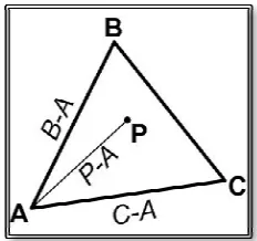
3.2.3 Point-In-Triangulation test

There are several mathematical algorithms and equations that can check

resides inside the triangle interior. In this thesis, the Barycentric Coordinates algorithm [19] was chosen. Barycentric coordinates are triples of numbers

to masses placed at the vertices of a reference triangle determine a point P, which is the

with coordinates (t1, t2, t3), as shown in

Figure 3.5:

Let the three points of the triang One of the points is chosen such that considered as relative to that point. Next, values to all the locations on the plane.

20

To increase the accuracy of estimated location of the sensor node, the triangle includes a smaller inner triangle that shares the same vertex defined by the location provides the same effect as candidate rings in the enhanced voting based scheme. As a result, the region at which the sensor node is most likely to reside is:

Inner Triangle. The inner triangle vertices can be defined using the

Triangulation test

mathematical algorithms and equations that can check whether a point triangle interior. In this thesis, the Barycentric Coordinates algorithm Barycentric coordinates are triples of numbers (t1, t2, t3) corresponding

masses placed at the vertices of a reference triangle ∆ABC. These masses then , which is the geometric centroid of the three masses and is identified

, as shown in Figure 3.5.

Figure 3.5: Barycentric coordinates [19].

three points of the triangle define a plane in space, as shown in is chosen such that we all other locations on the plane

considered as relative to that point. Next, basis vectors are needed to give coordinate values to all the locations on the plane. The two edges of the triangle that touch

To increase the accuracy of estimated location of the sensor node, the triangle includes a smaller inner triangle that shares the same vertex defined by the location candidate rings in the enhanced voting-based scheme. As a result, the region at which the sensor node is most likely to reside is:

Inner Triangle. The inner triangle vertices can be defined using the

whether a point triangle interior. In this thesis, the Barycentric Coordinates algorithm corresponding . These masses then of the three masses and is identified

and (B−A) are selected. Any point on the plane walking some distance along

(B−A) [15].

Figure 3.6:

With that in mind, we can des

According to the above equation, point if: u, v > 0, and u + v 1.

Given the coordinates of point to check whether the point P

Having two unknown variables

Solving for those two equations:

Where:

ny point on the plane can now be reached by starting at walking some distance along (C−A) and from that point walking further in the direction

Figure 3.6: Point in Triangle test [15].

we can describe any point on the plane as:

According to the above equation, point P can be inside the triangle ABC

the coordinates of point P, we can calculate u and v using the equation above resides inside the triangle or not, as shown below

Having two unknown variables u and v, we need two equations to solve for them:

r those two equations:

by starting at A in the direction

ABC if and only

using the equation above resides inside the triangle or not, as shown below [15]:

22

The point in triangle test can easily be programmed using the following pseudo code [15]:

− // Compute vectors w0 = (C−A)

w1 = (B−A) w2 = (P−A)

− // Compute dot products dot00 = dot(w0, w0) dot01 = dot(w0, w1) dot02 = dot(w0, w2) dot11 = dot(w1, w1) dot12 = dot(w1, w2)

− // Compute barycentric coordinates

invDenom = 1 / (dot00 × dot11 − dot01 × dot01) u = (dot11 × dot02 − dot01 × dot12) × invDenom v = (dot00 × dot12 − dot01 × dot02) × invDenom

− // Check if point is in triangle

return (u > 0) && (v > 0) && (u + v < 1)

3.2.4 The proposed secure range-free location discovery algorithm

Putting the triangle creation method and the point in triangle test together, the algorithm of a secure range-free location discovery is now defined. Using the example shown in Figure 3.7, the details of how this proposed algorithm works can be explained.

Figure 3.7: Proposed secure range

The voting process starts by identifying the guide point from the closest reference location received, in this example it would be point U. For each of the remaining location references, V and W, the inner and outer

described in section 3.2.b. The second step

reside inside the region defined by subtraction of shaded area shown in Figure

checking if any vertex of the cell is inside the shaded region using the Point test described in section 3.2.c.

After the sensor node processes all the location references, it selects the cells with highest vote, and uses their ge

node (point P’ in our example)

support iterative refinement as in the original scheme presented in [8, 9]. The cells with maximum vote will be quantized further into smaller cells and fed back into the voting process algorithm again to refine the estimated location results.

The proposed secure range the following pseudo code:

Proposed secure range-free location discovery scheme.

The voting process starts by identifying the guide point from the closest reference location received, in this example it would be point U. For each of the remaining location

inner and outer triangles would be created using the met described in section 3.2.b. The second step is the voting process of marking

region defined by subtraction of outer triangle from inner triangle (the Figure 3.7) and incrementing their vote by 1. This is done by checking if any vertex of the cell is inside the shaded region using the Point

test described in section 3.2.c.

node processes all the location references, it selects the cells with highest vote, and uses their geometrical centroid as the estimated location of the sensor

in our example). The secure range-free location discovery

support iterative refinement as in the original scheme presented in [8, 9]. The cells with uantized further into smaller cells and fed back into the voting process algorithm again to refine the estimated location results.

The proposed secure range-free location discovery scheme can be summarized in free location discovery scheme.

The voting process starts by identifying the guide point from the closest reference location received, in this example it would be point U. For each of the remaining location triangles would be created using the method the cells that from inner triangle (the is is done by checking if any vertex of the cell is inside the shaded region using the Point-In-Triangle

node processes all the location references, it selects the cells with ometrical centroid as the estimated location of the sensor free location discovery scheme can support iterative refinement as in the original scheme presented in [8, 9]. The cells with uantized further into smaller cells and fed back into the voting

24

− Receive location references {(X1, Y1, Hops1), (X2, Y2, Hops2), ...};

− Determine the extents of deployment field:

− Lower left corner = min. x-coordinate and y-coordinate values among the location reference;

− Upper right corner = max. x-coordinate and y-coordinate values among the location reference;

− Quantize the deployment field into small square cells;

− Select the location reference with min. hops to be the guide point.

− For each cell in quantized deployment field, initialize the voting value to 0; − For each location reference (Xi, Yi, Hopsi) {

o set outerTriangle (vertex=(Xi, Yi);

Height=(radioRange × Hopsi);)

o set innerTriangle (vertex=(Xi, Yi);

Side=(radioRange × (Hopsi-1));)

o for each cell in quantized deployment field {

perform PIT test on cell vertices;

if (PIT test returns TRUE for outerTriangle && FALSE for innerTriangle) increment cell vote by 1;

}

}

− highVoteCells = Get the set of cells with highest vote;

Chapter 4

I

T

R

This chapter explores the implementation of both enhanced voting-based and secure range-free schemes on Sun SPOT wireless sensors. The schemes were tested on a combination of actual SPOT and virtual SPOT sensors using Solarium, the emulation environment provided by Sun SPOT. Another set of tests that focused on security resilience under various types of attacks was performed using a simulation program developed for this purpose.

4.1

Implementation on Sun SPOTs and System Architecture

4.1.1 Overview on Sun SPOT wireless sensors

The Sun SPOT sensor device is a small, wireless, battery powered experimental platform. It is programmed almost entirely in Java to allow programmers to create projects that require specialized embedded system development skills. The hardware platform includes a range of built-in sensors as well as the ability to easily interface to external devices [16].

Figure 4.1:

4.1.2 Implementation system architecture

Both the enhanced voting-based and secure range implemented in Java as library

Sun SPOT runs an application that creates an instance of the

library and sets the type of location discovery scheme to be used in the deployed sensor network. Figure 4.2 shows a block diagram of the system architecture at each

sensor.

The Sun SPOT sensor runs three main threads: receiving, transmitting and location discovery. These three threads run simultaneously as soon as the SPOT sensor is deployed. The receiving thread is responsible

messages from surrounding sensors and beacon nodes. Once the receiving thread gets a location reference message, it checks

in the location reference list. If the location reference

simply ignored, otherwise, the receiving thread retrieves the hops count and other routing information about the source of this location reference from the SPOT routing manager The hops count is then attached

location reference list.

The transmitting thread is responsible location to its surrounding neighbors.

location estimator class, and in

sensor (maximum radio range, location discovery scheme, initial quantization resolution). Once the SPOT sensor has received enough location reference

thread triggers the location discovery process and blocks both receiving and transmitting threads until the location is estimated.

26

Figure 4.1: Sun SPOT sensor [16].

Implementation system architecture

based and secure range-free location discovery schemes implemented in Java as library classes to be used in Sun SPOT wireless sensors.

ns an application that creates an instance of the secure location discovery location discovery scheme to be used in the deployed sensor shows a block diagram of the system architecture at each

SPOT sensor runs three main threads: receiving, transmitting and location discovery. These three threads run simultaneously as soon as the SPOT sensor is deployed. The receiving thread is responsible for keeping track of location reference messages from surrounding sensors and beacon nodes. Once the receiving thread gets a location reference message, it checks to see if this location reference is already included in the location reference list. If the location reference has already been received

simply ignored, otherwise, the receiving thread retrieves the hops count and other routing information about the source of this location reference from the SPOT routing manager

is then attached with the location reference coordinates to be added to the

The transmitting thread is responsible for broadcasting the SPOT’s estimated location to its surrounding neighbors. The location discovery thread creates an instance of location estimator class, and initializes it with the basic information about the SPOT sensor (maximum radio range, location discovery scheme, initial quantization resolution). Once the SPOT sensor has received enough location references, the location discovery on discovery process and blocks both receiving and transmitting threads until the location is estimated.

location discovery schemes are to be used in Sun SPOT wireless sensors. Each location discovery location discovery scheme to be used in the deployed sensor shows a block diagram of the system architecture at each Sun SPOT

SPOT sensor runs three main threads: receiving, transmitting and location discovery. These three threads run simultaneously as soon as the SPOT sensor is keeping track of location reference messages from surrounding sensors and beacon nodes. Once the receiving thread gets a this location reference is already included ived, then it is simply ignored, otherwise, the receiving thread retrieves the hops count and other routing information about the source of this location reference from the SPOT routing manager. oordinates to be added to the

Figure 4.

The secure location discovery library contains either enhanced voting-based scheme, or range

is the locationEstimator class which handles all the interfaces with the upper layer of threads.It also manages the location references, quantization of

and cells vote generation. When a

class it is initialized with the SPOT’s radio coverage range, initial quantization resolution and the type of location discovery scheme to be used to estimate the SPOT’s location.

The locationEstimator class receive and stores those location references in

locationEstimator receives enough location references (

minimum of three points are required to build a triangle), it sends a ready signal to the location discovery thread. The location discovery thread returns a request to the locationEstimator to initiate a location discovery process. The location discovery process

Figure 4.2: System architecture block diagram.

secure location discovery library contains the necessary classes to perform based scheme, or range-free scheme. The main class in the library locationEstimator class which handles all the interfaces with the upper layer of the location references, quantization of the deployment field map When a Sun SPOT creates an instance of the locationEstimator class it is initialized with the SPOT’s radio coverage range, initial quantization resolution and the type of location discovery scheme to be used to estimate the SPOT’s location.

The locationEstimator class receives location reference from the receiving thread and stores those location references in the Location Reference List. When the Estimator receives enough location references (three or more reference since a minimum of three points are required to build a triangle), it sends a ready signal to the location discovery thread. The location discovery thread returns a request to the ionEstimator to initiate a location discovery process. The location discovery process necessary classes to perform free scheme. The main class in the library locationEstimator class which handles all the interfaces with the upper layer of deployment field map Sun SPOT creates an instance of the locationEstimator class it is initialized with the SPOT’s radio coverage range, initial quantization resolution, and the type of location discovery scheme to be used to estimate the SPOT’s location.

28

location references. The deployment field map is then quantized into a set of cells, each with a zero vote value. The locationEstimator passes the list of location references and cells set to the location discovery scheme specified by the Sun SPOT. The location discovery scheme generates the votes on the cells set and returns the set to the locationEstimator, which in turn extracts the cells with maximum votes value and calculate the geometrical centroid (center of gravity for a mass) of those cells to be the estimated location.

Iterative refinement is performed by the locationEsitmator to increase the accuracy of the estimated location. This is done by quantizing the set of cells with maximum votes further into smaller sub-cells and feeding the new sub-cells back to the location discovery scheme for votes’ generation. The process continues until the difference between two consecutive estimated locations are less than 5%. At this point, the locationEstimator returns the estimated location to the location discovery thread to be broadcasted by the transmitting thread.

4.2

Test Cases and Simulation Results

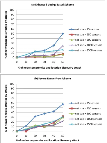
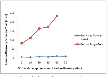
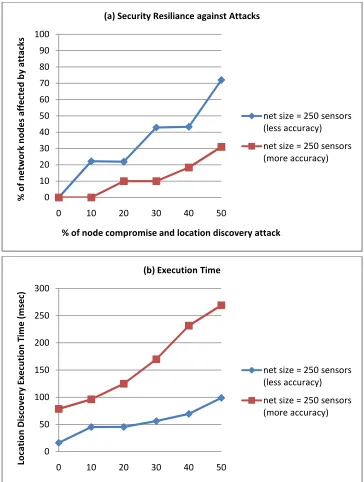
This thesis presents two sets of test cases. The first is implemented on Sun SPOTs wireless sensors to check the location discovery schemes accuracy and behavior. The second test case is implemented on a simulation program to investigate the security resilience of the location discovery schemes to various degrees of node compromise and location discovery threats.

4.2.1 Test on Sun SPOTs and Solarium

The first experiment is to test the accuracy of the estimated location of both the enhanced voting-based scheme and the secure range-free scheme by comparing the distance error between the sensors’ actual location and their estimated location. The test was performed on Sun SPOT wireless sensors using the Solarium emulator. Solarium is a Java™ application that can be used to remotely manage a network of Sun SPOTs. With Solarium, SPOTs can be discovered and the life-cycle of the applications running on those devices can be managed [17].

Receiving and sending via the radio is also supported

own address and can broadcast or unicast to the other virtual SPOTs. If a shared basestation is available, a virtual

When a virtual SPOT emulator code in a Squawk

over a socket connection with the virtual SPOT GUI when the SPOT application changes the RGB value of an LED to the virtual SPOT GUI code

value. Likewise when the user clicks

mouse, Solarium sends a message to the emulator code that the which can then be noticed by the SPOT application.

the Emulator architecture [17]

Figure 4.3: Block diagram of emulator architecture in Solarium

Each virtual SPOT has its own Squawk VM host computer. Each Squawk VM

of the SPOT library. This allows the

applications running on the host computer, such real SPOTs via radio if a shared basestation is running

The experiment was implemented

on a network of 9 virtual SPOTs, 3 of those SPOTs were beacon nodes and th sensor nodes, as shown in Figure

Receiving and sending via the radio is also supported. Each virtual SPOT is assigned its and can broadcast or unicast to the other virtual SPOTs. If a shared

a virtual SPOT can also interact over radio with real SPOTs a virtual SPOT is created in Solarium, a new process is started to run the

a Squawk Virtual Machine (VM). The emulator code communicates over a socket connection with the virtual SPOT GUI code in Solarium. For example when the SPOT application changes the RGB value of an LED, that information is passed to the virtual SPOT GUI code which updates the display for that LED with the new value. Likewise when the user clicks on one of the virtual SPOT's switches using the

Solarium sends a message to the emulator code that the switch has been clicked, noticed by the SPOT application. Figure 4.3. shows a block diagr

[17].

Block diagram of emulator architecture in Solarium [17]

Each virtual SPOT has its own Squawk VM running in a separate process on the Squawk VM also contains a complete host-side radio stack as part allows the SPOT application to communicate with other SPOT applications running on the host computer, such as other virtual SPOTs, using sockets or real SPOTs via radio if a shared basestation is running [17].

implemented twice, once for each location discovery scheme, a network of 9 virtual SPOTs, 3 of those SPOTs were beacon nodes and th

Figure 4.4.

. Each virtual SPOT is assigned its and can broadcast or unicast to the other virtual SPOTs. If a shared SPOT can also interact over radio with real SPOTs [17]. new process is started to run the . The emulator code communicates code in Solarium. For example information is passed updates the display for that LED with the new RGB one of the virtual SPOT's switches using the switch has been clicked, a block diagram of

[17].

running in a separate process on the side radio stack as part SPOT application to communicate with other SPOT other virtual SPOTs, using sockets or

Figure 4.4:

The experiment starts with the beacon nodes broadcasting their locations to the other sensor nodes. Each sensor node receives location references from its nei

estimates its location accordingly

surrounding neighbors. After several rounds of modifying t