City, University of London Institutional Repository
Citation
: Song, Guangming (1988). An application of computer aided design and
computer aided draughting techniques to gearing.. (Unpublished Doctoral thesis, The City University)This is the accepted version of the paper.
This version of the publication may differ from the final published
version.
Permanent repository link:
http://openaccess.city.ac.uk/19505/Link to published version
:
Copyright and reuse:
City Research Online aims to make research
outputs of City, University of London available to a wider audience.
Copyright and Moral Rights remain with the author(s) and/or copyright
holders. URLs from City Research Online may be freely distributed and
linked to.
AN APPLICATION OF <no1Pl1I'ER AIDED DESIGN
AND COMPUTER AIDED DRAUGHTING TECHNIQUES TO GFARING
B Y -GUANGMING SONG
A Thesis Submitted for the Degree of Doctor of Philosophy
THE CITY UNIVERSITY
Department of Mechanical Engineering The City University
London E.C.l
IMAGING SERVICES NORTH
Boston Spa, WetherbyWest Yorkshire, LS23 7BQ www.bl,uk
CONTAINS
Table of Contents
List of Tables and Illustrations Acknowledgements
Abstract Symbols Chapter 1
1.1 1.2 1.3 1.4 Chapter 2 2.1 2.2 2.2.1 2.2.2 2.2.3 2.3 2.4 Chapter 3 3.1 3.2 3.3 3.4 3.5 3.6 3.7 Chapter 4
Introduction
Computers in Engineering Design Process in Engineering Computer-Aided Design
This Thesis
Computing System and Software Development System Requirements
Choice of Language for Implementation High-Level Programming Language
Assembly Language Graphics Package
Selection of Computer Operation Mode Program Structure
Tooth Number Calculations Introduction
Continued Fractions Conjugate Fractions Statement of Problem Method Description Program Description Examples and Discussion Gear Tooth Generation
4.1 Introduction 62 4.2 Generation of Involute Gear Teeth by Rack-Form
Cutter 63
4.3 Determination of Tooth Profile by Graphical
Generation Method 67
4.4 Calculation of positions of the Cutter Tooth Profiles
4.5 Program Description
Chapter 5 Calculation of Gear Tooth Profile 5.1 Introduction
5.2 Calculation of Rectangular Coordinates of Involute Profile
5.3 Calculation of the Pressure Angle at the Starting Point of Involute Profile
5.4 Calculation of Rectangular Coordinates of Tooth
69 72 76 76 76 78
Fillet 83
5.5 Calculation of Rectangular Coordinates of the
Maximum Bending Stress position on the Gear Tooth 86 5.6
Chapter 6 6.1 6.2 6.2.1.1 6.2.1.2 6.2.1.3 6.2.2
Program Description Gear Train Design Introduction
Strength Design Theory and Approach
Gear Rating Standards National Standards
Effects of Standards on Design ISO Approach
Detailed Analysis of Gear Strength
6.2.3 Estimation of Major Dimensions for Specified Requirements
6.3 Geo.metric Calculation
6.4 Design of Gears Operating on Specified Centre
Distances 103
6.4.1 Adjusting the Helix Angle to Obtain a Specified
Centre Distance 103
6.4.2 Selecting the Suitable Combined Modification
Coefficients to Achieve a Desired Centre Distance 106 6.4.3 Altering the Tooth Sum to Suit a Given Centre
Distance 109
6.5 Optimum Distribution of Gear Ratio for Double
Reduction Gearing 113
6.5.1 General Considerations of Gear Ratio Distribution 113 6.5.2 Basic Equations for Equal Contact Strength
Requirements 6.5.3 6.5.4 6.5.5 6.5.6 6.5.7 6.5.a 6.6
Basic Equation for Lightest Weight Basic Equation for Minimum Size
Basic Equation for Standardised Centre Distances Basic Equation for Splash Lubrication
Ten Methods to Distribute Gear Ratio for Double-Reduction Gearing
Example
Description of Gear Design Program
Chapter 7 Application of Finite Element Techniques to Gear Tooth Stress Analysis
114 117 120 122 123 125 130 132 139
7.1 Introduction 139
7.2 Finite Element Method 141
7.3 Point of Application of Load for Maximum Bending
Stress 143
7.4 Selection of Tooth Model 144
7.5 Determination of the Maximum Tooth Root Bending
7.6 Gear Tooth Geometry and Finite Element Grid Description
7.7 7.8 7.9 Chapter 8 8.1 8.2 8.2.1 8.2.2 8.2.3 8.2.4 8.2.5 8.2.6 8.2.7 8.2.8 8.2.9 8.3 8.4 8.5 Chapter 9 9.1 9.2 9.2.1 9.2.2 9.2.3 9.2.3.1 9.2.3.2 9.2.3.3 9.2.3.4
Data Preparation Results
Summary
Shaft Design Introduction Design Theory
Determination of Loading Preliminary Physical Design Materials for Shafting
Design for Combined Stresses Further Physical Design
Checking for Fatigue Strength Checking for Static Strength Checking for Rigidity
Vibration and Critical Speeds of Shafts Shaft Model
Design Approach Program Description Bearing Selection Introduction
Bearing Selection Procedure Force Analysis
Selection of Bearing Types Selection of Bearing Sizes Determination of Bearing Life Calculation of Dynamic Capacity Calculation of Equivalent Load Calculation of Static Capacity
9.3 Chapter 10 10.1 10.2 10.3 10.3.1 10.3.2 10.3.3 Chapter 11 Chapter 12 12.1 References
Description of Bearing Selection Program Computer Aided Draughting
Introduction
Basic Geometric Construction Techniques Description of Draughting Programs Gearbox Schematic Drawing Program Gear Working Drawing Program Shaft Working Drawing Program Design Techniques
Conclusions
Future Development
195 202 202 203 212 212 214 217 219 224 224 226
Appendices 235
Appendix A An Example of the Use of the Program GCHECK 236 Appendix B A Typical Data File for LUSAS 241 Appendix C An Example of the Use of the Program SDESIGN 243 Appendix D An Example of the Use of the Program BSELECT 251 Appendix E Complete Record of a Single-Reduction Gearing
LIST OF TABLES AND ILLUSTRATIONS
Page Table 1.1 Potential for Computer Utilisation in a Design
Process 10
Table 3.1 Tooth Combinations to Provide a Gear Ratio of
2.94643 + 0.0001 57
Table 3.2 Tooth Combinations to Provide a Gear Ratio of
2.94643 ~ 0.0001 (Derived from [63]) 59 Table 3.3 Tooth Combinations to Provide a Gear Ratio of
0.70711 + 0.00005 60
Table 3.4 Tooth Combinations to Provide a Gear Ratio of
2.236068 + 0.000001 61
Table 6.1 Centre Distance a (JBl130-70) 123 Table 6.2 Gear Design Results by Using Different Gear Ratio
Split Methods 131
Table 6.3 Theoretical Number of Solutions Obtained from
Gear Design Program 132
Table 7.1 Results of FEM Calculation for Tooth Surface
Stress at Points along the Tensile Tooth Fillet 152 Table 8.1 Allowable Deflections and Slopes of Shafts 167 Table 9.1 Representative Bearing Design Lives 186
Table 9.2 Ball Bearing Reliability Factor f¢b and Roller
Bearing Reliability Factor f¢r 188 Table 9.3
Table 9.4 Table 9.5 Table 9.6 Table 9.7 Table 9.8
Load-Application Factor f 189
P Temperature Factor f
t 189
Table 10.1 Statistics on Some Typical Engineering Drawings 204 Figure 1.1 The Iterative Design Process 5 Figure 1.2 Flowchart Showing Stages in a Design Process 7 Figure 2.1 Two Presentations of the Same Data 28 Figure 2.2 Flowchart for Gearbox Computer Package 33 Figure 2.3 Main Menu of the Gearbox Design Programs 34 Figure 2.4 Sub-menu 1 of the Gearbox Design Programs 34 Figure 2.5 Sub-menu 2 of the Gearbox Design Programs 35 Figure 2.6 Sub-menu 3 of the Gearbox Design Programs 35 Figure 3.1 Convergents of a Simple Continued Fraction 42 Figure 3.2 Flowchart for the Program TOOTHN 46 Figure 3.3 Location of Pl/ql and P
2/q2 without Solution 47
Figure 3.4 Location of P2/Q2 within the Tolerance T and R 48 Figure 3.5 Flowchart for the subprogram CONTIN 50 Figure 3.6 Flowchart for the subprogram CONJUG 51 Figure 3.7 Internal Expansion between PI/OI and P2/02 52 Figure 3.8 External Expansion on the Left Side beyond
AlB
to C/D
Figure 3.9 External Expansion on the Right Side beyond
AlB
toc/n
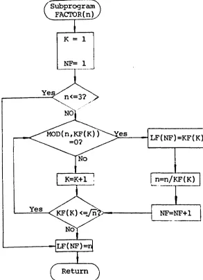
Figure 3.10 Flowchart for the subprogram FACTOR
53
54 55 Figure 4.1 Rack-Form Gear-generating Cutter 63 Figure 4.2 Generation of Spur Gear by Rack-Form Cutter 64 Figure 4.3 Displacement of a Rack-Form Cutter 65 Figure 4.4 Rolling Motion between Rack-Form Cutter and
Gear Blank
Figure 4.5 Two Relative positions of Rack-Form Cutter and Gear Blank
Figure 4.6 Rack-Form Cutter with Protuberance Figure 4.7 Flowchart of Gear Tooth Generation
68
Figure Figure Figure Figure Figure Figure
4.8 Gear Tooth Generation from a Rack-Form Cutter 4.9 Gear Tooth Generation from a Rack-Form Cutter
with a Protuberance Tip
5.1 Rectangular Coordinates of Involute Profile 5.2 Dimension of a Typical Basic Rack
5.3 Interference Points of Gears
5.4 Terminal Point K of the Straight Portion of Basic Rack Profile
Figure 5.5 Pressure Angle at the Starting Point of Involute Profile without Undercutting
Figure 5.6 Pressure Angle at the Starting Point of
Invo-75 75 77 78 79 80 80
lute Profile with Undercutting 81
Figure Figure Figure
5.7 Rectangular Coordinates of Tooth Fillet 5.8 Maximum Root Tensile Stress position
5.9 Gear Tooth Drawing from the Program GTPROF Figure 5.10 Gear Tooth Grid and Information from the
Program GTPROF
Figure 6.1 Flowchart of Design for Specified Centre Distances
Figure 6.2 Longitudinal Dimension L of Double-reduction Gearing Figure Figure Figure Figure Figure Figure Figure
6.3 Splash-lubricated Double-reduction Gearing 6.4 Typical Double-Reduction Gear Systems 6.5 Schematic Flowchart of Gear Train Design 7.1 Point of Contact for Maximum Bending Stress 7.2 Tooth Model for Finite Element Stress Analysis 7.3 Finite Element Grid for Gear Tooth
7.4 Principal Stress Contours of Gear Tooth Figure 7.5 Results of FEM Calculation for Tooth Surface
Stress at Points along the Tensile Tooth
Figure 8.1 Figure 8.2 Figure 8.3
Figure 8.4 Figure 8.5 Figure 9.1 Figure 9.2 Figure 9.3
Figure 9.4 Figure 10.1
Figure 10.2 Figure 10.3 Figure 10.4 Figure 10.5 Figure 10.6 Figure 10.7 Figure 10.8 Figure 10.9 Figure 10.10 Figure 10.11 Figure 10.12 Figure 10.13 Figure 10.14 Figure 10.15 Figure A.1
Fillet 153
Fillet Radius of a Shaft 162
Chamfering of Component Mounted on a Shaft 163 Assembly Requirement for Fillet Radius on a
Shaft 163
Shaft in Deflected Position 168
Stepped Shaft Model 170
Bearing Loads Acting on Radial Thrust Bearings 192
Bearing Selection Flowchart 196
Flowchart of Finding the First Possibly Suitable Bearing in the Given Series
Sample Output of Information on Bearing 313 Graphic Outputs from the Twenty Geometric Construction Subroutines Used on a Calcomp 1051 Drum Plotter
200 201
207 Examples of the Use of Subroutine DIMEN 209 Schematic Diagram of CIRKEY Arguments 209
Samples of CALL CIRKEY 211
Schematic Diagram of SKSHADE Arguments 211 Examples of the Use of Subroutine SKSHADE 211 Interference between Gear and Shaft 213
A Gear Oiled by a Pinion 213
Spoked Gear 215
Webbed Gear 215
Solid Gear 216
Size e of Pinion 216
Integral Pinion Shaft 216
Figure B.l
Figure C.l Figure C.2 Figure D.l
Typical Data File for Gear Tooth Stress Analysis Using LUSAS
Schematic of Sample Shaft Checking
Typical Application of the Program SDESIGN Typical Application of the Program BSELECT Figure E.l Complete Record of a Single-Reduction Gearing
Design Process
241 243 244 251
254 Figure E.2 Computer Output of Gearbox Schematic 275 Figure E.3 Computer Output of Integral Pinion Shaft Working
Figure E.4 Figure E.5
Drawing
Computer Output of Gear Working Drawing
Computer Output of Output Shaft Working Drawing
I grant powers of discretion to the University Librarian to allow this thesis to be copied in whole or in part without further reference to me. This permission covers only single copies made fur study purposes, subject to normal conditions of acknowledgement.
ABSTRACT
The thesis describes the development of a computer-aided design and computer-aided draughting package of industrial gearboxes for transmitting power between shafts having parallel major axes. The package mainly consists of the following functions:
(a) Determination of gear tooth numbers from the properties of continued and conjugate fractions
(b) Generation of gear teeth by a rack-type cutter
(c) Calculation of gear tooth profile and production of gear tooth grid for finite element stress analysis
(d) Detailed strength analysis and design of a spur or helical, external or internal, standard or modified, single- or double- reduction gear set based on the ISO gear standards (e) Shaft design and analysis
(f) Bearing selection and analysis
(g) Production of the working drawings of the main gearbox components.
Symbols
For the purposes of this thesis the following symbols apply.
Symbol Designation a centre distance b facewidth
reference diameter of pinion addendum of basic rack
m module
normal module
rotational speed of pinion tip radius of basic rack
r reference radius
reference radius of pinion reference radius of gear base radius
base radius of pinion base radius of gear
u gear ratio
x addendum modification coefficient
normal addendum modification coefficient
z tooth number
tooth number on pinion tooth number on gear
nominal tangential force at reference circle K resultant load factor
KA application factor
KFa
transverse load factor for bending stress KF8 face load factor for bending stressUnits
. -1 m1n
Designation
transverse load factor for contact stress face load factor for contact stress
dynamic factor
transverse load distribution factor face load distribution factor
resultant factor for bending stress resultant factor for torsional stress
actual safety factor for bending stress (against breakage)
SFmin minimum demanded safety factor for bending stress (against breakage)
SH actual safety factor for contact stress
SHmin minimum demanded safety factor for contact stress TI pinion torque
Y
F tooth form factor for bending stress Y
NT life factor of a test specimen Y
S stress correction factor for bending stress Y
ST stress correction factor of a test specimen
=
2.0 YRrelt relative surface condition factor for bending stress
Y
x
size factor for bending stress Ys
helix angle factor for bending stressY relative sensitivity factor for bending stress orelt
Z resultant factor for contact stress ZE elasticity factor for contact stress
ZH zone factor for Hertzian pressure at pitch point for contact stress
ZL lubricant factor for contact stress ZN life factor for contact stress
Units
Symbol Designation
roughness factor for contact stress speed factor for contact stress
work hardening factor for contact stress size factor for contact stress
helix angle factor for contact stress contact ratio factor for contact stress
Ct pressure angle at reference cylinder
normal pressure angle at reference cylinder transverse pressure angle at reference cylinder transverse pressure angle at pitch cylinder
B helix angle at reference cylinder
n
mechanical efficiency~a facewidth factor (FW/CD)
~d facewidth factor (FW/reference diameter)
~a equivalent factor for bending stress
~1 equivalent factor for torsional stress
bending endurance limit for symmetrical cycle bending stress amplitude
tooth root bending stress
endurance limit for bending stress endurance limit for contact stress mean bending stress
torsional endurance limit for symmetrical cycle torsional stress amplitude
mean torsional stress
Chapter 1
INTRODUCTION
1.1 ~uters in Engineering
Digital computers have revolutionized engineering practice, just as they have other aspects of modern life. Computers have become an absolutely essential tool in all phase of engineering, from research and development to marketing and management. The engineer of a generation ago would probably not even recognize many of today's routine engineering activities that rely heavily on digital computers. Even after four decades the computer
revo-lution shows no sign of slowing. New discoveries and improvements in computer-technology continue at such a pace that many products and techniques in the computer field become obsolete within a few years time.
Moreover the microelectronics revolution has stimulated the development of powerful personal microcomputers. Complete computer systems are now relatively inexpensive. Along with being low-cost, this equipment is also more reliable and simpler to use than its computing ancestors. The ready availability of these devices is enabling a large number of engineers to become familiar with computing techniques and to become aware of their potential for effective design.
1.2 Design Process in Engineering
The design process involves applications of technology for the transformation of resources, to create a product that will satisfy a need in society. The product must perform its function in the most efficient and economic manner within the various constraints that may be imposed. It is the ability to design an efficient product that sets apart the successful designer.
As a general rule, there are three main types of design work, each of which requires a different level of intellectual ability and creativity.
Primarily,. there is the adaptation of existing designs which require only minor modification, often in the dimensions of the product. This type of work represents a large proportion of the total design work undertaken. The designer engaged entirely in this type of work needs only the basic technical skills and will not appreciate the nature of the design process unless other work is undertaken.
considerable and the final product may be very different from the original item. In certain cases the use of an existing design may make the solution more difficult to obtain, and the level of ability and time spent by the designer may be considerable. This is sometimes called adaptive design.
Finally, the most demanding work concerns the design of a new product that has no precedent. This needs a high level of ability and relatively few designers will be engaged in this type of activity. It is sometimes referred to as creative design.
The design problem gives the designer the opportunity to utilise and develop his creative skills to their full extent. In order to select a technique or idea that will provide a solution to the problem, the designer requires both practical experience and a depth of knowledge. He must then be able to relate widely different elements and recognise their mutual adaptability. Ultimately, a truly creative solution will only emerge if the designer can apply open-ended thinking and can also appreciate
alternative solutions and strategies.
The overall design process usually has five stages of development:
stage (1) Identifying the Problem:
Stage (2) Feasibility Study:
Having identified a need for the product, the next stage is to conduct a basic feasibility study. It must be physically possible to produce the product, it must be economically viable and it must be acceptable. If the alternative solutions cannot be physically realised, the project will not proceed unless the problems concerned are overcome by appropriate prior development work.
Stage (3) Preliminary Design:
At this stage, having defined the need or the problem and ascertained that a solution may be feasible, it becomes necessary to select the best approach to the problem. Where several alternatives exist they should all be examined in an unbiased manner, with equal thoroughness. It may be found at this stage that a solution which appeared possible eaorlier can now not be achieved. At the conclusion of the preliminary design phase i t must be decided which approach to the final solution is to be examined further and is most likely to be adopted. It should be remembered that this choice is not irreversible and results obtained later may require that this approach is abandoned and an alternative is developed.
This stage uses combinations of the three fundamental design methods described as follows:
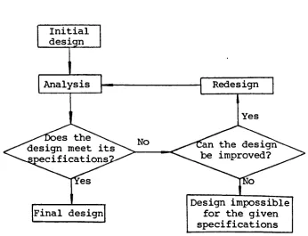
(a) The Iterative Design Method:
design constraints. If it fails to do so, then it is modified on the basis of further information obtained from the analysis, and reana1ysed until the design can meet the specification, or until the designer is convinced that this design is not feasible within the given constraints.
The iterative design process, illustrated in flow chart form in Figure 1.1, therefore contains three main activities:
(1) Initial Design (2) Analysis
(3) Redesign.
Analysis Redesign
Yes
No
Design impossible Final design for the given
specifications
Figure 1.1 The iterative design process
(b) The Direct Design Method:
[image:24.564.119.465.324.589.2]words, a design is produced directly by analysis. This process implies that a design can be defined by a parametric representa-tion, and that interactions between parameters are known.
(c) The Design Selection Method:
A design process may yield a number of solutions which all satisfy given constraints. This is applicable to the situation where the design constraints themselves contain one or more variables. In this situation the selection of the final design, given the performance characteristics for each design, is largely a matter for human judgement by compromising performance as it is affected by design constraints.
Stage (4) Detailed Design:
An approach to the solution has been chosen and a full detailed design is now prepared. All components and systems are fully specified and all inservice requirements should be defined. A complete set of production drawings is also prepared. At this stage less alternatives are available to the designer and a significant economic commitment is usually required. Any major revisions, or the decision to abandon an approach entirely, should be made before progressing to the next stage. If not, considerable investment will be wasted. It may be that events outside the designer's control may cause the product to become unacceptable at a later stage. This possibility should be minimised by constant feedback and continual re-evaluation of the problem identification and feasibility studies.
Stage (5) Production:
between the designer and the production engineer.
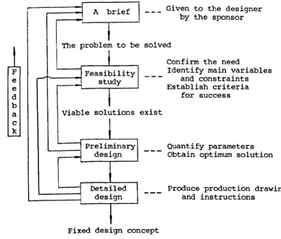
One of the clearest and simplest analyses of the stages in a design study can be summarised as shown in Figure 1.2.
F e e d b a c k
J A brief
~
The problem to be
l
Feasibility study
i
Viable solutions
Preliminary design
Detailed design
Given to the designer by the sponsor
solved
exist
Confirm the need
Identify main variables and constraints Establish criteria
for success
Quantify parameters Obtain optimum solution
Produce production drawings and instructions
Fixed design concept
Figure 1.2 Flowchart showing stages in a design process
1.3 ~ter-Aided Design
The meaning of 'Computer-Aided Design' (CAD) has changed several times in its past twenty years or so of history. For some time, CAD was almost synonymous with finite element structural analy-sis. Later, the emphasis shifted to computer-aided draughting
[image:26.552.99.501.139.480.2]of three-dimensional objects, (this is typical in many branches of mechanical engineering). In [26], CAD is considered as a discipline that provides the required know-how in computer hardware and software, in systems analysis and in engineering methodology for specifying, designing, implementing, introducing and using computer based systems for design purposes.
To be brief, CAD can simply be defined as a technique in which the designer and machine are blended into a problem-solving team, intimately coupling the best characteristics of each. The result of this combination works better than either the designer or the computer would work alone, and by using a multi -discipline approach it offers the advantage of integrated team-work.
CAD implies by definition that the computer is not used when the designer is most effective, and vice versa. It is, therefore, the marriage of the characteristics of each which is so important in CAD. These characteristics affect the design of a CAD system in the following areas:
(a) Design Construction Logic:
The use of experience combined with judgement is a necessary ingredient of the design process. The design construction must therefore be controlled by the designer. This means that the designer must have the flexibility to work on various parts of the design at any time and in any sequence, and be able to follow his own intuitive design logic rather than a stylised computer
logic.
(b) Information Handling:
detailed design is complete, information must in turn be output to enable the design to be manufactured. The human brain is able to store information in an intuitively ordered manner, but its storage capacity is limited, and the information is not all retained as time passes. By contrast, computers have no ability to organise data intuitively but have large permanent storage capacities. Information storage should therefore be carried out by the computer under the direction of the designer.
The output of manufacturing information, from the detailed design stage of the design process, usually involves the production of drawings. This is a time-consuming, laborious and error prone process when carried out manually but is quite suitable for execution by the computer. It is therefore desirable to allow the computer to generate as much production information as possible, so freeing the designer from repetitious work at all stages of the design process.
(c) Modification:
Design descriptive information must frequently be modified to make correction of errors, to make design changes, and to produce new designs from previous ones. The computer has the ability to detect those design errors which are systematically definable: whereas man can exercise an intuitive approach to error detection. For example, the computer can calculate the torque capacity of a shaft, whilst a designer can tell from experience and judgement that the shaft is too small.
(d) Analysis:
A computer is very good at performing those analytical calcula-tions of a numerical analysis nature which the designer finds time-consuming and tedious. As much as possible of the numerical analysis involved in the design should be done by the computer, leaving the designer free to make decisions based on the results of this and his own intuitive analysis.
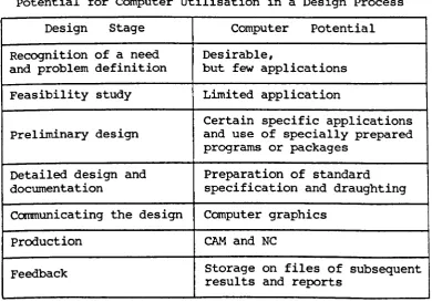
The stages in the design process and the possible uses of a computer are illustrated in Table 1.1 [66J.
Table 1.1
potential for Computer Utilisation in a Design Process Design Stage Computer Potential Recognition of a need Desirable,
and problem definition but few applications Feasibility study Limited application
Certain specific applications Preliminary design and use of specially prepared
programs or packages
Detailed design and Preparation of standard documentation specification and draughting ccmnunicating the design Computer graphics
Production CAM and NC
Feedback Storage on files of subsequent results and reports
[image:29.562.106.497.342.615.2][66]. CAD is being increasingly adopted by architects, shoe-makers, surgeons, industrial designers, etc. It is only a matter of time until CAD becomes a standard tool in all design offices, progressing in tandem with a steady adaptation of the work procedures there. Not only the indu~trial nations but also the developing countries are beginning to realize that CAD will be an essential constituent of practically all industrial enterprises in the near future [26].
1.4 This Thesis
Industrial gearboxes are commonly used in mechanical systems such as in machine tools, cranes and automotive applications and re-present an important area of mechanical engineering manufacture. The design of a gear set is a reasonably difficult problem which involves the satisfaction of many design constraints. It is the job of the designer to specify the major geometrical features of a gear set in order to achieve known requirements. This design process is iterative and time-consuming by hand. Currently more exacting analytical techniques are being advocated to establish more reliable rating information and hence a reduction in factors of safety. Inevitably the associated calculations become more complex and the volume of data required increased. These make gearing design a design work which is especially suited to computers.
The application of a computer to the design of gearboxes would offer many significant advantages:
(3) The calculations can be based on more accurate theory and do not have to be over-simplified in the interest of speed. (4) The calculations can cover a wide range of alternative
designs very quickly.
(5) The calculations can be performed iteratively to examine the sensitivity of performance to a large number of design dimensions and other design parameters such as material, accuracy, etc., thus allowing better optimisation of design.
The application of computer techniques to gearing design has to date been a fairly well explored field. Allan and Forgie [6] show the feasibility of integrating design functions using computers, citing gear train as an example. Cockerham and Waite [16] present a computer-aided procedure for the design of a 200 pressure angle spur or helical gear train based on strength and wear calculations outlined in BS436:1940 [10]. The program varies the module, face width, and gear ratio to obtain an acceptable design, in which no account has been taken of non-standard or internal gears. Tucker [82] and Estrin [32] look more closely at the gear parameters, such as addendum ratio and pressure angle, and outline procedures for varying a standard gear mesh to obtain a more favourable gear set. Savage, Coy and Townsend [69] establish an optimal design procedure for standard spur gear pairs. The procedure utilizes standard gear geometry and optimizes the number of pinion teeth to obtain the minimum centre distance for a given application of specified speed reduction and
process can be simplified by using a computer.
In these computer programs, some concentrate only on specialised aspects of gear design, while others claim to have taken a more integrated approach to the subject. Invariably each package will contain some special facility or feature. To justify the development of a new gear design package based on systematic comparison of functional and other merits with existing packages, is difficult due to the different programming approaches adopted in addition to the problems of acquiring the various packages. The author has endeavoured to produce a package capable of expansion to cover a much wider range of design functions than already exists.
This approach has been used to develop a suite of modular programs organised into a package for the design of
sing1e-reduction and double-sing1e-reduction gear units. The main functions and features of the package are as follows:
(1) Determination of tooth numbers which satisfy a particular gear ratio within a specified tolerance from the properties of continued fractions and conjugate fractions.
(2) Generation of gear teeth by a rack-type cutter, which may be derived from different national standard or nonstandard basic racks.
(3) Calculation and drawing of gear tooth profile, which may be generated by the rack cutter of different national standards.
positions for the gear tooth stress analysis using finite element methods.
(5) Detailed geometric calculations of a spur or helical, external or internal, standard or nonstandard gear pair, which provide the designer with the considerable informa-tion necessary for strength analysis, manufacturing, and inspection such as pitch diameters, contact ratios, pressure angles at the highest points of single tooth pair contact, base tangent lengths and diameters over pins, and information on undercutting, interference and topping.
(6) Detailed strength analysis and design for a spur or helical, external or internal, standard or modified, single reduction or double reduction gear train based on the international gear rating standard IS0/DlS6336 [39]. In design situations, many alternative solutions, if required, will be presented to the designer by adopting different facewidth factors and helix angles (for helical gears). Moreover, when a double reduction gearbox is employed, the designer may also choose different gear ratio split methods on the basis of different requirements of application. Therefore, much more alternative design solutions may be obtained.
(7) Design and analysis of a stepped shaft supported by two bearings for combined bending and torsional strength,
fatigue strength, rigidity, and vibration.
(8) Selection and analysis of a roller contact bearing based on basic dynamic capacity and basic static capacity.
(9) Production of the working drawings of the main gearbox components such as gears and shafts.
interactive features of the program permit a designer to be involved in crucial stages of the design process, provide considerable flexibility with the designer to apply his experience and skill to the problem solving, and enable him to quickly explore several alternative design conditions in order to achieve a more optimal design solution.
(11) The design programs are implemented on the IBM personal computer and its compatible machines with eGA, EGA, or Hercules display adapter as these computers are relatively cheap to buy and therefore more readily accessible to a designer.
(12) The design programs can present the designer with far more information than is normally required and the documentation for the design is also well prepared by the computer output.
(13) The package is not only useful as a practical design tool in industry but also helpful as a teaching resource for instruction in the gear design process in education.
The author has also studied the maximum tooth root bending stresses using finite element method and compared the results with those using the ISO gear standard.
l I' '.
;
; ~
,
I I
I
Chapter 2
caotPt1I'ING SYS'l'D1 AND SOFTWARE DEVELOPMENT
2.1 BystemRequirements
The computer software described in the thesis is broadly divided into two types of programs, namely design programs and draughting programs. The draughting programs will be described in detail in Chapter 10. The hardware used by the author in preparing the design programs covers three different kinds of computer systems that are widely used across all industries, education, and in the home. These micros are
(1) IBM PC/AT compatible microcomputer which has 1 MB of memory, a 20 or 40 Mb hard disk, a mathematical co-processor, a Hercules display adapter, and a dot matrix printer:
(2) IBM Personal Computer which has 640 KB of memory, a 20 Mb hard disk, a math co-processor, an Enhanced Graphics Adapter, and IBM Graphics Printer:
(3) Amstrad PC15l2 computer which has 512 KB of memory, two disk drives with 360 KB capacity, no math ccrprocessor, a Colour Graphics Adapter, and a dot matrix printer.
2.2 Choice of Language for Implementation
2.2.1 High-level Programming Language
Programming in the early days of computing was tedious in the extreme. Programmers required a detailed knowledge of the instructions, registers, and other aspects of the central processing unit (CPU) of the computer for which they were writing code. In the 1950s it became increasingly apparent that this form of programming was highly inconvenient although it did enable the CPU to be used in a very efficient way.
These difficulties spurred a team led by John Backus of IBM to develop the first ever high-level language, Fortran. The language was indeed simple to learn, as it was possible to write mathema-tical formulae almost as they are usually written in mathemamathema-tical texts. (in fact, the name Fortran is a contraction of Formula Translation.) This enabled working programs to be written faster than before, for only a small loss in efficiency. We thus see that Fortran was an innovation, as the first high-level language.
But Fortran was revolutionary as well as innovatory. Programmers were relieved of the tedious burden of using machine language, and were able to concentrate more on the problem in hand. Perhaps more important, ·however, was the fact that computers became accessible to any scientist or engineer willing to devote a little effort to acquiring a working knowledge of Fortran: no longer was it necessary to be an expert on computers to be able to write application programs.
for a variety of applications include scientific and engineering computation, simulation and modeling, process control, business and accounting, and so on. The most widely used programming languages at present are FORTRAN, Pascal, C and BASIC [23].
The choice of which programming language should be used to create a particular program is of crucial importance, not only because of possible changes of program, but also because of possible changeovers to other computer systems. High-level programming languages are not machine specific. Programs written in them (source program) are converted into machine language instructions by compilers or interpreters (program translators). When changing from one computer to another, the user does not, therefore, have to change the source program, but only the compiler or interpreter. A programming language is also chosen on how well suited the programming language features are matched to the work that the particular program has to accomplish. In the course of time new languages have been developed, and where they were demonstrably more suitable for a particular type of application they have been adopted in preference to Fortran for that purpose. Fortran's superiority has always been in the area of numerical, scientific, engineering, and technical applications, and there is still no significant competitor in these fields.
following a period of public comment and further work to take the comment into account, the final standard be published in about 1989, just allowing for the x in Fortran 8x to have the value 8.
Fortran is a compiler language: the source program written by the programmer must be translated (compiled) into machine language instructions by the compiler. Although the draft Standard for Fortran 8x has now been published and the final standard might be published in 1989, history has shown the software industry in general to be very slow to adopt new standards. It is unlikely that a Fortran 8x compiler will be available in the near future.
The gearbox design programs of the package are written in Fortran 77. The compiler used for translating (compiling) the programs is the Microsoft (MS) Fortran Optimizing Compiler (Version 4.01) developed and marketed by the Microsoft Corporation of Bellevue, Washington [55, 56]. The MS-Fortran compiler is specifically designed for compiling a Fortran 77 source program on the personal computer. Several versions of this compiler are in use, with Version 4.01 (copyright 1987) being the latest by this time.
allows the user to link Microsoft FORTRAN programs with 8086 assembly-language programs and Microsoft C and Pascal programs.
2.2.2 Assembly Language
Programs are often judged by their display quality and visual design alone. Most application programs take pains to make themselves attractive and easy to use. They do not simply display one line after another, scrolling 'old lines off the top of the screen: they display their messages and results in specific areas of the screen. They also control the color and brightness of what they display, and often they assign special meanings to certain keys. In general, control of the display screen, like most other computer operations, can be done in three ways:
(1) By using the high-level programming language services: (2) By using the ANSI driver services:
(3) By using the ROM-BIOS video services.
In the beginning, DOS did not provide adequate video services. But starting with version 2.00, it became possible to perform the needed screen work through the DOS services enhanced with the ANSI driver program, also known as ANSI.SYS. This program uses a set of commands that, when translated, will perform just about anything the screen is capable of doing. In general, the ANSI driver is only active when we deliberately introduce it into DOS through the CONFIG.SYS file that DOS loads during the start-up operation. The specific command in the CONFIG.SYS file that is used to activate the ANSI.SYS driver is :
DEVICE = ANSI.SYS
When ANSI.SYS is installed, it recognizes certain character sequences as being command sequences. All ANSr.SYS command sequences begin with an escape character whose ASCII value is 27. ANSI.SYS command sequences are not displayed on the screen. ANSI.SYS can carry out four types of commands: erase all or part of the display screen, control cursor position, set display modes and attributes (color, underscore, blinking, etc.), and reassign character strings to individual keys on the keyboard [71]. By using the ANSI driver, for example, the following subroutine written in Fortran 77 is used to clear the entire screen and set
the cursor to the home position.
SUBROUTINE CLS
PRINT'(IX,2A)',CHAR(27),'[2J'
END
assembly-language interfaces into the ROM-BIOS services, the ANSI driver makes the most crucial BIOS-type services available to any programming language. Furthermore, it can be a great benefit to programmers who want to write programs that are not tied to the PC family, but instead will work on any DOS computer using the
ANSI driver.
Despite these apparent advantages, the use of the ANSI driver commands in our programs is not a good idea. For one thing, it requires that the ANSI driver be installed in any computer that our programs are used on, which adds considerably to the instructions that we have to prepare to accompany the programs. It is difficult enough trying to explain the setup and use of our programs to both novices and experts, without adding extra layers of complexity, such as the explanation of how to install the ANSI
driver.
A further argument against the use of the ANSI driver is that it is not available under all circumstances. For example, IBM's windowing system, Topview, does not support the features of the ANSI driver, so programs that require the driver cannot be used with Topview. This may well turn out to be true with other windowing environments as well.
But most important of all is the fact that, compared to the BIOS service, the ANSI driver is pathetically slow in generating full screen output. Unless there is very little screen output to be displayed, the ANSI driver is just too slow to be satisfactory.
fundamental services that are needed for the operation of the computer. For the most part, the BIOS controls the computer's peripheral devices, such as the display screen, keyboard, and disk drives. The ROM-BIOS is a collection of machine-language routines. Conceptually, the ROM-BIOS services are sandwiched between the hardware and the high-level languages (including the operating system). In effect, this means that the BIOS works in two directions in a two-sided process. One side receives requests from programs to perform the standard BIOS input/output services. These services are invoked by our programs with a combination of an interrupt number (which indicates the subject of the service request, such as video services) and service number (which indicates the specific service to be performed). The other side of the BIOS communicates with the computer's hardware devices (display screen, disk drives, etc.), using whatever detailed command codes each device requires. This side of the BIOS also handles any hardware interrupts that a device generates to get attention. For example, whenever we press a key, the keyboard generates an interrupt to let the BIOS know. There are twelve ROM-BIOS interrupts in all. Most of the interrupts are tied to a
group of subservices that actually do the work. The video services interrupt 16 (hex 10) has sixteen subservices that provide nearly all the services that are needed to generate display-screen output, control the cursor, and manipulate screen information [59]. In order to make direct use of the ROM-BIOS services from our programs, we need to create an
CODE
CLS
CLS CODE
SEGMENT 'CODE' ASSUME CS:CODE PUBLIC CLS PROC FAR PUSH BP MOV BP,SP MOV AH,OFH
INT lOH MOV AH,OOH INT lOH MOV SP,BP POP BP RET
ENDP ENDS END
:save caller's frame pointer :save stack pointer
:get current video mode
irequest video service
iset video mode
irequest video service ;restore stack pointer
:restore caller's frame pointer :return to caller
Assembly language and high-level language each have their own benefits and drawbacks. Compared with high -level language, assembly language requires more work to write because it requires more lines of program code to accomplish the same end, and it is more error-prone because it involves lots of niggling details. One important drawback of assembly language is that it requires more expertise to write than most high-level languages. However, there are important advantages to it as well: assembly language programs are usually smaller and run faster (Table 2.1 shows the size and speed comparison between of the two subroutines described above), because we use our skills to find efficient ways to perform each step, while high-level languages generally carry out their work in a plodding unimaginative way. Also, using assembly language we can tell the computer to do anything it's
Table 2.1
capable of doing because assembly language provides us with full access to the ROM -BIOS and DOS services, while high -level languages normally don't give us a way of performing all the tricks that the computer can do. Broadly speaking, we can say that high-level languages let us tap into 90 percent of the computer' skills, while assembly language lets us use 100 percent, if we're clever enough. This illustrates an important point in the creation of professional-quality programs: often the best programming is done primarily in a high-level language (such as Fortran or Pascal), with assembly language used as a simple and expedient means to go beyond the limits of the high-level
language.
By using the ROM-BIOS and DOS services through the assembly language, many general-purpose subroutines are developed by the author. They will be applied to the package to enhance its performance. The following is general descriptions of some
subroutines.
BEEP Beep
CGA Set video mode for Colour/Graphics Adapter CHKKBD Check whether a key has been pressed or not
CLS Clear the entire screen and return the cursor to home position
CLSWD Clear a specified window (part of the screen) OOSVER Get OOS version number
FREESP Get disk free space
HOME Return the cursor to home position
KEYIN Returns the equivalent ASCII code if a key is pressed at the keyboard
LINEV Draw a vertical line
LOCATE Move the cursor to a given line and column of the screen LOCERA Erase characters from a given position to the end of
line and return the cursor to the given position MONO Set video mode for Monochrome Adapter
PROMPT Display characters with certain attribute such as blink-ing reverse video
RCURXY Report current cursor position PRTSC
~Gm
SBOX
Print screen
Move the cursor right one column Draw a box of single-line type
Graphics Package
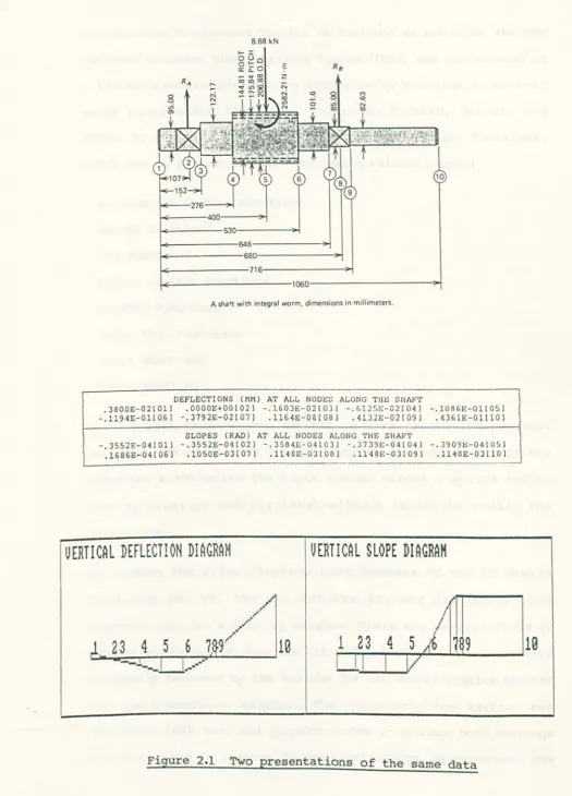
Computer graphics is the most versatile and most powerful means of communication between a computer and a human being. When the results of computation are presented using graphics, complex data is easier to digest and analysed, and relationships become immediately evident. Integrating graphics into data analysis can have positive effect on design quality of product. Compare the two data presentation formats shown in Figure 2.1. The graphic representation of the data will quickly get the attention of the designer, who will locate the critical positions of the shaft.
8.68 kN
~~ o u .
o~o E
R8
0::0::0
RA :::
-
""""""..
"" Z": Lri18
~~N ~
~----530----~~ ~---~6---~~
~---680---~
k---716--->~
~---1000---~~
A shaft with integral worm, dimensions in millimeters.
DEFLECTIONS (NN) AT ALL NODE~ ALONG TilE SIIAFT
.3600E-02101J .OOOOE~OOI02J -.1603E-02!03J -.612SE-02[04J -.1086E-Ol[OSJ
-.1194E-Ol(06) -.3792E-02[07] .1164E-08!081 .4132E-02!091 .4361E-Ol[lOJ
SLOPES (RAD) AT ALL NODES ALONG THE SHAFT
-.3552E-04101J -.3552E-04(02) -.3584E-04(03) -.3739E-04(04) -.3909E-04105)
.1686E-04!061 .1050E-03(07) .1148E-031061 .1l46E-03(09) .1l40E-03!101
UERTICAL DEFLECTION DIAGRAM
UERTICAL SLOPE DIAGRAM
lQ
[image:47.554.10.535.39.768.2]Computer Graphics Development Toolkit [34].
The Graphics Development Toolkit is designed to run under the IBM Personal Computer Disk Operating System (DOS), and implemented as a linkable subroutine library supported by bindings to several major programming languages, including Fortran, Pascal, and BASIC. It contains a long list of graphics and text functions, which may be presented in the following related groups:
workstation Control Functions Paging Functions
Pel Functions
Cursor Control Functions Graphic Functions
Alpha Text Functions Input Functions Error Handling
The Graphics Development Toolkit is also device-independent. Therefore, we can direct our application program output to any supported workstation (an input and/or output graphics device such as displays and printers) without having to modify the
application.
Monochrome Adapter can operate only in text mode, using a stored set of ASCII alphanumeric and graphics characters and displaying them in only one color. To overcome these limitations, some hardware manufacturers have come up with variations of the IBM Monochrome Adapter, such as the popular Hercules display adapter, which successfully combines the graphics (but not the color) capabilities of the Color/Graphics Adapter with the higher-quality text display of the Monochrome Adapter. The Enhanced Graphics Adapter can create graphics on the monochrome screen in a similar way.
The type of display adapter that might be used has an important effect on program design. The Graphics Development Toolkit only supports Color Graphics Adapter and Enhanced Graphics Adapter, but does not support Hercules display adapter. To make up this weakness, a memory resident utility has been introduced, which simulates Color Graphics Adapter with Hercules Monochrome Adapter, and allows the package to be able to run in graphics mode using Hercules Monochrome Adapter.
2.3 Selection of Computer Operation Mode
In general, there are two modes of computer operation, namely batch mode and interactive mode. Batch mode is the traditional way of using a computer. For any design problem where computer aid is being considered it should be the first method to be examined, as in many cases it will be found that it is perfectly adequate and that the more sophisticated techniques of usage are not necessary.
computer starts processing a set of data it continues to comple-tion or until some error situacomple-tion occurs when it terminates. The user has no method of correcting such errors during that run. He must wait until he receives his output, alter his input and run the program again from the beginning.
Interactive mode allows the user to communicate directly with a computer, usually send data or instruction via the keyboard and receive output from the display screen or printer. By these means, the user and the computer can work interactively, modifying and improving the design and correcting errors without having to wait for the final results to be presented to him. This mode is an essential part of a computer-aided design practice.
An analysis of mechanical engineering products reveals that they are made from basic entities such as structures and machine elements. The machine elements can be divided into gears, shafts, bearings, seals, connecting rods and other similar components. In addition, basic situations will exist, such as stress concentra-tion, vibraconcentra-tion, lubrication and contact stress. Properties of materials are involved implicitly in all the basic entities and situations. Each entity and situation is a design segment and the designer when synthesizing a possible solution will include a number of these segments which will interact with each other. Therefore, the most efficient way of using the computer in the mechanical engineering design process would appear to be to allow the designer and computer to interact in a conversational mode to evolve an acceptable design by providing the designer with conversational programs and a personal computer system or a
results of analysis on-line and the designer making decisions and choices based on judgment from the computer's answers. In this way the user is able to interrogate more data and analyse more trial runs, so giving him much more information on which he himself can make the design decisions.
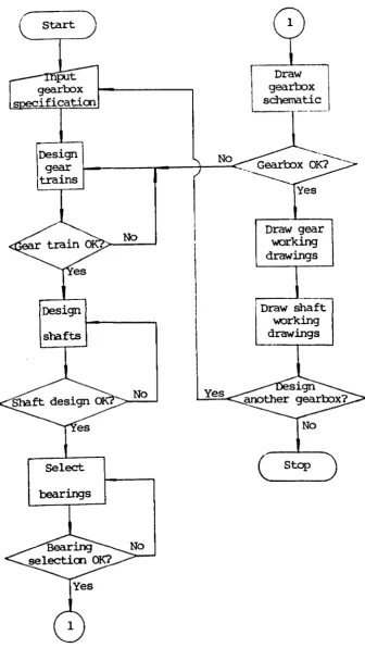
The gearbox design programs developed operate in an interactive mode. Figure 2.2 indicates an outline of the whole gearbox design and draughting package when it is linked with a computer. It will
be noticed that the computer is essentially used to complement the designer. At the end of each activity, the designer is able to study the design results before processing to the next stage or re-running the programs if he is not satisfied with the results. In this way, the designer is given considerable freedom to reach an acceptable solution using his ability and experience. The designer's skill at making important design judgements is fully employed while time-consuming and unproductive iterative calculations are left to the computer. A more automated approach involving less interaction with the designer would in general be unsatisfactory for dealing with such design problems.
2.4 Pro9ram Structure
Start
Draw
gearbox
schematic
' - - - - ---.
[DeSign
' _____
gear I - - _ - - - - . . _ - - + - - c Gearbox OK?
trains
---No
Design
sha.fts
No
Select
bearings
Yes
Yes
Draw gear
1NOl"king drawings
[
raw shaft
working drawings
No
stop
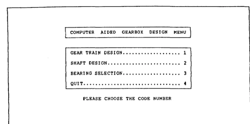
[image:52.564.142.478.83.690.2]COMPUTER AIDED GEARBOX DESIGN MENU
GEAR TRAIN DESIGN . . . 1
SHAFT DESIGN .•••.••.•.••.••••.•.••.• 2
BEARING SELECTION ••..•••.••••••••••• 3
QUIT ••••.••••.••••••••••.•.••••••••• 4
PLEASE CHOOSE THE CODE NUMBER
Figure 2.3 Main menu of the gearbox design programs
COMPUTER AIDED GEAR DESIGN MENU
FIND TOOTH NUMBERS FOR SPECIFIED GEAR RATIO .•..••.• 1
GENERATE GEAR TOOTH .•...••..•...•••...• 2
DRAW GEAR TOOTH PROFILE •••.•.••••.••..•••••••••••.• 3
PRODUCE FINITE ELEMENT GRID OF GEAR TOOTH .•.••••••• 4
CALCULATE GEOMETRICAL SIZES OF GEAR PAIR •••••••••.• S
CHECK CONTACT AND BENDING STRENGTHS OF GEAR SET •••• 6
DESIGN GEAR TRAIN •••••.•••••.•••••••••••••••••••••• 7
OUIT··· •.••••..••••••• 8
[image:53.564.89.501.126.330.2]PLEASE CHOOSE THE CODE NUMBER
COMPUTER AIDED SHAFT DESIGN ~
CHECK SHAFT .•••••••..••.••
3
...
1 DESIGN SHAFT . • . • . • . . . . • . • . . . • • . • . 2"UIT ••...•••••.••.•...•..•.•.••. 3
PLEASE CHOOSE THE COvE NUMBER
L--_ _ _ _ _ _ _ _ _ _ _ _ _ _ _ _ _ _ _ _ _ _ _ _ _ . _ _ _ _ _ _ _ _ _ _ _ _ _ _ _ _ _ _ - - '
Figure 2.5 Sub-menu 2 of the gearbox design programs
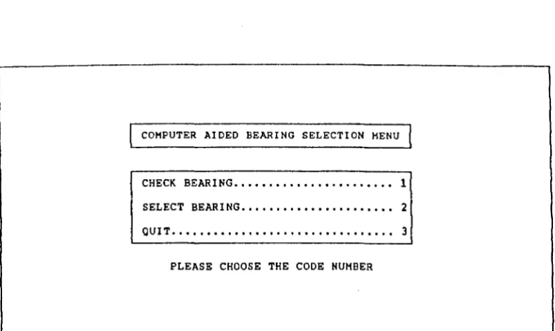
COMPUTER AIDED BEARING SELECTION MENU
CHECK BEARING ••••••••••••••••••••••• 1
SELECT BEARING •••••••••••••••••••••• 2 QUIT •••••••••••••••••••••••••••••••• 3
PLEASE CHOOSE THE CODE NUMBER
[image:54.564.93.504.126.336.2] [image:54.564.105.508.444.684.2]When this computer software runs, input data is typed on the keyboard and output appears on the screen. Both input data and output results will also be recorded in computer files, which may be printed as a permanent record of the design process.
The design prograns have many inbuilt user features, which are designed to make the programs as foolproof as possible and to give clear unambiguous instructions to the user. These features are as follows:
(1) An input data language easily interpreted by the designer is employed.
(2) Inputting data takes the form of making a choice wherever possible.
(3) Making a choice by typing a single key without having to press <RETURN>.
(4) There are a number of safeguards made available against wrong entries. For example, the input routine will ignore any alphabetic entry when the numeric entry is expected. Thus accidental typing errors are prevented from causing program failure.
(5) Detection and warning of inconsistent data and data which could cause program failure. For instance, in the bearing selection program the ent~y of a bore diameter less than zero or not a standard value will result in BEEP or the response
NO BEARING HAS A XXX MM BORE DIAMETER. THE STANDARD BORE DIAMETERS NEAR TO THE REQUIRED VALUE ARE XXX AND XXX MM. PLEASE INPUT DATA AGAIN.
program.
(6) The input data can be corrected by using the editing facility of the program.
(7) The output is clearly labelled and self-explanatory.
(8) Whenever the user is unsatisfied with the design results, he can modify any of the original parameters without having to terminate the design process and re-enter all items of data so that he is able to see the effect of the change immediately.
(9) Optional displaying of data and/or results such as the detail information on gear pair design.
(10) optional printing of graphical output such as shaft slope and deflection diagrams.
As the software is fully interactive, all the user needs to do is to sit in front of a computer, start the programs and then input data in reply to requests displayed on the screen in front of him. Ideally, the user should not need to know any more about the programs than what he is told by means of the screen. However, it is reasonable for the program writer to assume that the user will have a general knowledge related to gear design, shaft design, and bearing selection. Because it is so quick to input the data to a problem the user is encouraged to seek alternative
Chapter 3
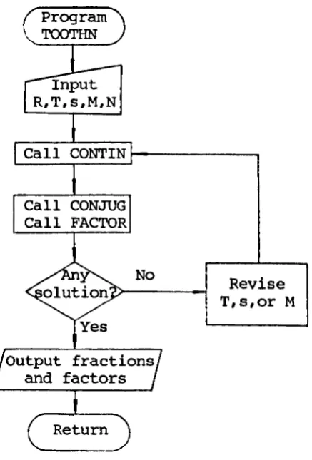
TOOTH NUMBER CALCUIATIONS
3.1 Introduction
In most problems in gear design, the velocity ratio has a tolerance of a few per cent, and in those cases there is rarely any difficulty in selecting numbers of teeth with an acceptable ratio. On the other hand, it is sometimes necessary, in the setting-up of machine tools for screw cutting, spiral milling, gear cutting, and so on, to discover at least one combination of 'change gears' with a velocity ratio that departs from the specified figure by no more than 1 part in 100,000 or so.
So close an approximation in a single pair of gears would usually demand that each of them should have several hundreds of teeth with the disadvantage of low load capacity in relation to diameters and width. This difficulty is avoided by using a two-stage train and then any velocity ratio up to about 8 to 1 can be closely approximated without using any gear with more than 100 teeth. Where exceptionally fine tolerance is imposed, a three-stage train may be considered, as it offers a much larger number of approximating ratios.
A great deal of work has been done in investigating means of solving problems of this type with very fine tolerance. Tables of change-gear combinations are published by some machine-tool manufacturer. That issued by the Pfauter Company, for example, comprises more than 200 pages listing upwards of 26,000 combinations covering ratios between 0.1 and 1.0. The greatest departure from any ratio that might be specified is about 20 in 100,000 for ratios near 0.1, 3 in 100,000 for ratios around 0.5, and 1 in 100,000 for ratios of nearly 1.0, but will in many cases be less [50]. These combinations probably satisfy all practical machine-tool requirements, but they do not exhaust all the possibilities. If a special case demands a closer approximation than tabulated combinations afford, or if a table of change-gears is not available, recourse to other methods becomes necessary. McComb and Matson [48] list five methods, all of which involve cut-and-try procedures. Spotts [73] describes a sixth cut-and-try technique. orthwein [63] develops a microcomputer program, which is founded upon the theorem that a denumerable infinity of rational numbers can be found between any two real numbers whose difference is greater than zero.
The following sections show that some properties of continued fractions and conjugate fractions will greatly contribute to the solution of the problem, and offers a direct means for finding the required number of teeth on each gear. A numerical method is outlined and three examples of its use terminate the discussion.
3.2 Continued Fractions