Autonomous robot patrolling of a sparsely populated unknown environment

(1)

Rochester Institute of Technology

RIT Scholar Works

Theses Thesis/Dissertation Collections

11-1-2010

Autonomous robot patrolling of a sparsely

populated unknown environment

Patrick LaRocque

Follow this and additional works at:http://scholarworks.rit.edu/theses

This Thesis is brought to you for free and open access by the Thesis/Dissertation Collections at RIT Scholar Works. It has been accepted for inclusion in Theses by an authorized administrator of RIT Scholar Works. For more information, please [email protected].

Recommended Citation

(2)

Autonomous Robot Patrolling of a Sparsely Populated

Unknown Environment

by

Patrick J. LaRocque

A Thesis Submitted in Partial Fulfillment of the Requirements for the Degree of Master of Science in Computer Engineering

Supervised by

Associate Professor, Department of Computer Engineering Dr. Shanchieh Jay Yang Department of Computer Engineering

Kate Gleason College of Engineering Rochester Institute of Technology

Rochester, New York November 2010

Approved By:

Dr. Shanchieh Jay Yang

Associate Professor, Department of Computer Engineering Primary Adviser

Dr. Andres Kwasinski

Assistant Professor, Department of Computer Engineering

Dr. Sonia Lopez Alarcon

(3)

Thesis Release Permission Form

Rochester Institute of Technology

Kate Gleason College of Engineering

Title: Autonomous Robot Patrolling of a Sparsely Populated Unknown

Environment

I, Patrick J. LaRocque, hereby grant permission to the Wallace Memorial Library

re-porduce my thesis in whole or part.

Patrick J. LaRocque

(4)

Dedication

To my wife Jessica without whom none of this would have been possible. To my family,

(5)

Acknowledgments

I am grateful for all of the guidance and dedication that Dr. Yang has provided to help me

through this thesis process. I would also like to thank Dr. Kwasinski and Dr. Lopez

(6)

Abstract

The increasing availability and affordability of autonomous robots has expanded their uses

for many new applications, such as exploration, surveillance and threat containment. Most

research considers a team of a large number of robots that contain global information. This

work explores distributed and low overhead algorithms for patrolling and threat

contain-ment within a region sparsely populated with few robots. The robots patrol the area without

the global knowledge of the region, but each is equipped with an omni-directional range

finder and a positioning system for keeping track of its location and metering distance

and directions of events. This study presents the extent of effectiveness and limitations of

utilizing a limited number of robots patrolling an unknown wide-spread region.

A set of three algorithms was developed. All algorithms assume the use of artificial

potential fields (APFs) for collision avoidance with other robots and the walls as well as

to approach the threat. The algorithms differ in two ways; whether or not the robots have

a limited memory of past events and the way the robots maneuver from one patrol target

location to another. The next patrol target location can be derived randomly or based on

past events. The past events include previously sensed robot locations, target locations, and

walls. The algorithms are analyzed in terms of the time it takes for the robots to detect and

neutralize threats within the surveillance region. Simulations via MATLAB are conducted

to investigate the tradeoffs due to factors such as the number of robots, the size of the

region, and the frequency of threats. The results show that the three algorithms perform

comparably on average, achieving reasonable effectiveness given the inherent limitations

(7)

List of Figures

2.1 Ladybug Force Geometry[18] . . . 9

2.2 Initial Robot Configuration, Trajectories, and Final Configuration[18] . . . 10

2.3 Autonomous Robot Cleaning Path Planning Techniques[10] . . . 12

2.4 Combined Covering Path Planning[10] . . . 13

3.1 Robot Operational Flow Chart . . . 17

3.2 Effect of Forces on Robot Movement . . . 19

3.3 Artificial Potential Field Forces . . . 21

3.4 Robot Spiraling Towards Patrol Target Location . . . 24

3.5 Threat Hand Off . . . 27

3.6 Patrol Target Creation Step 1 . . . 31

3.10 Fading Effect of Historical Point . . . 36

4.1 Robot Movement Simulation . . . 43

5.1 Normalized Time to Target vs. Wall Fading Method for all three Robot Fading Methods using the History Algorithm with 45◦ Spiral Towards PTL 47 5.2 Normalized Time to Target vs. PTL Storage Method . . . 49

5.3 Histogram of Normalized Time to Target Values . . . 53

5.4 Histogram of Normalized Time to Target Values with Log Scale . . . 54

5.5 Histogram of 95% of Normalized Time to Target Values with Log Scale . . 55

5.6 Normalized Time to Target vs. Region Size with 95% of Values . . . 57

5.7 Normalized Time to Target vs. Number of Robots with 95% of Values . . . 59

5.8 Normalized Time to Target vs. Number of Threats with 2s Threat Elimina-tion Time with 95% of Values . . . 61

(10)

5.10 Square Surveillance Region . . . 64 5.11 Slightly Irregular Surveillance Region . . . 64 5.12 Complex Convex Surveillance Region . . . 65 5.13 Normalized Time to Target vs. Surveillance Region Shape with 95% of

Values . . . 66

5.14 Normalized Time to Target vs. Number of Stored PTLs with 95% of Values 68

(11)

List of Tables

3.1 Threat to Robot Force . . . 22

3.2 Robot to Robot Force . . . 22

3.3 Wall to Robot Force . . . 23

3.4 Exploratory Force . . . 23

3.5 Step Threshold . . . 25

3.6 Historical Point Types and Number Stored . . . 28

3.7 Patrol Target Distance . . . 30

3.8 Fading Patrol Target Distance . . . 35

3.9 Memory Usage . . . 38

4.1 Experiment Parameters . . . 41

5.1 Normalized Time To Target . . . 46

5.2 Common Experiment Parameters . . . 51

5.3 Simple 1000 Run Experiment Parameters . . . 51

5.4 Simple 1000 Run Experiment Results . . . 52

5.5 regionSizeto Region Area Mapping for Moderately Difficult Shape . . . . 56

5.6 Region Size Experiment Parameters . . . 57

5.7 Number of Robots Experiment Parameters . . . 58

5.8 Threat Arrivals Experiment Parameters . . . 60

5.9 Surveillance Region Shape Experiment Parameters . . . 65

5.10 Number of Stored PTLs Experiment Parameters . . . 67

(12)

Chapter 1

Introduction

1.1

Motivation and Background

Robotic platforms have become cheaper and more available over the last several years. The

increased availability has not only given rise to manufacturing and military robots, but also

for robots to handle common household chores[10]. Given the common usage of robots

for various tasks, many researchers have investigated how to allow robots to make better

decisions with less external control. Many of these scenarios use robots controlled remotely

like UAVs, while others are completely autonomous.

Autonomous robots are a particularly interesting area of research due to their

resem-blance to animals. The realization of the biological link gave rise to the study of robot

motion by imitating real animal behavior. Two such examples are flocking and swarms.

Flocks of birds move together like a super-organism. The benefits to birds include

protec-tion in numbers, allowing them to individually avoid detecprotec-tion by predators, as well as to

improve energy efficiency while traveling. These same benefits can be extended to robots

that mimic this behavior.

Threat containment and surveillance are active areas of research with military

applica-tions as well as security implicaapplica-tions. Many algorithms exist utilizing autonomous robots

to achieve these goals. Many of these are handled with teams of robots where movement

is dictated in one of two fundamentally different ways. Team management can be

(13)

robots are all controlled by a central overseer, often someone with a global view of the field

and knowledge of every task needed to be completed. Decentralized strategies are harder

to implement but have the benefit of randomly deployable robots that can remain dormant

and complete tasks when triggered by external stimuli. In these scenarios the robots act

completely autonomously, making decisions and forming behaviors based upon their own

sensor readings or global knowledge of the environment. They decide independently how

to move or what action to take. Autonomous robot research is further divided into

algo-rithms that require global knowledge and those that only rely on the sensor readings of the

robot. Some algorithms actually bridge this gap by allowing the robots to communicate

with each other wirelessly and share sensor knowledge.

1.2

Problem Statement

The fundamental task of a majority of the areas of autonomous robotic research has to do

with the robot mobility. Path planning is non-trivial with research on the subject spanning

decades. Given a large surveillance region with only a few low cost robots to cover the

area, what is the best path planning algorithm? Is it completely random, or should the

robot intelligently make decisions on how to proceed? With global knowledge of a fixed

environment at the start of a scenario, the obvious solution is to statically map out the

best route to a Patrol Target Location (PTL). What will happen, however, if the robots are

dropped in a region they are completely unfamiliar with? Will the random direction model

of movement yield the best results? Or can a more intelligent algorithm based on past

sensing history improve coverage? This research will attempt to answer these questions.

1.2.1

Scenario

Imagine the scenario where robot agents are dispersed in an area with no knowledge of their

environment and only limited sensing capabilities. Furthermore, the robots are only able

(14)

only advanced feature is a positioning system so that each robot will be able to remember

where it has been.

These robots are given the task of surveillance of this unknown area that is much larger

than their sensing range. The robots will continually explore the region and must not settle

out and become stationary, but instead keep looking for threats. The threats are toxins that

can appear in one concentrated area. These toxins could have fallen from the sky or could

be moving with the wind across the surveillance region. The robots’ job is to seek out the

threats and neutralize them without directions sent from a central controlling agent. While

being entirely autonomous, the robots will also operate without any global knowledge of

the environment. All calculations performed are based on events sensed only by the local

hardware to the robot. It is important that the robots plan their paths effectively through

the environment to explore new areas and avoid obstacles. Not only must this algorithm

be simple and efficient, but it must be able to run with the limitations of simple low cost

hardware available today.

1.3

Technical Issues

There are several issues that need to be overcome in order to achieve a comprehensive

al-gorithm that will be able to succeed in all of the goals in the described scenario. The factors

that will affect the robot movement and their interactions need to be decided. Obviously,

a minimum amount of stimuli and memory requirements are best in order to keep the

per-spective robot platforms at a minimal cost. Algorithms for the path planning and object

detection must be simple in order to keep the cost of processing low and limit the power

requirements needed. Memory constraints also effect the algorithms; a minimum amount

of data should be stored at any given time. This keeps the cost of the memory components

low as well as processing requirements low, allowing each robot to iterate over smaller data

(15)

1.3.1

Robot Limitations

Sensing the environment is not a simple task. Omni-directional sensors are commonly used

in autonomous robots to negate the need to rotate in place to sense the environment in every

direction. It is not necessary to artificially limit the sensing capabilities of a robotic system

to those of a human. The robot need not look around but instead be able to simultaneously

”see” in every direction. Expensive sensors like lidar can give a rapid and very adequate

mapping but are not feasible for a multi-robot deployment. Infrared (IR) sensors positioned

all around the robot can achieve the same effect with perhaps less resolution but at a much

lower cost. Using IR sensors will only give the distance and direction in which objects are

detected.

The robot in this study will have the ability to determine its position based on the

readings from the positioning system but will not know where the location is in reference

to anything else. This will be overcome when the robot has explored the surveillance region

and detects several objects. The positions of the last several locations that the robot had

sensed in the environment will be stored in local memory on the robot. The simple robots

that will be simulated in this work have very limited memories, therefore they will not be

able to store the locations for everything over time. Much of the memory will be consumed

in the calculation of the forces and their effects on the robot.

The drive system on the robot is not considered to be omni-directional, similar to the

limitations of the sensing capabilities. The robot must turn in place in order to move in the

new desired direction based on its sensory information. Due to the robot’s ability to sense

in every direction simultaneously, a robot can travel forward or reverse equally effectively.

Therefore, the most a robot will need to rotate is 90 degrees.

1.3.2

Environment and Threat Arrival

The problem this research attempts to solve involves a large sensing region within which

(16)

region so that their sensing ranges overlap and so no gaps are allowed where threats could

appear. This approach would be completely infeasible due to the high cost of the many

robots. The field would become so saturated with robots that any other use of the region

would become hindered. Since the threats rarely occur and can appear at any time in any

random location, it is not necessary to have many robots patrolling the region. Only one is

necessary to neutralize a threat at a time, so from a practical point of view it is unnecessary

to have more robots than there could possibly be threats at any given time. The robots will

eventually get to the threats and neutralize them.

1.4

Contribution

This research provides an important analysis of three different algorithms for movement

and path planning in a large region with few robots. Their performance is analyzed with

(17)

Chapter 2

Related Work

This thesis work was completed after an extensive search into the state of the art in

au-tonomous research. Several areas of related research are highlighted in the following

sec-tions as well as motivation for completing this work.

2.1

Robotic Platforms

There are many different robotic platforms capable of achieving the task described here.

Many of these platforms, however, have been mostly utilized to achieve group tasks in a

centralized manner. The Robotics Research Group of the DAEIMI University of Camino

used an experimental setup comprised of several Khapera II robots manufactured by

K-Team[16]. These commercially available robots have omni-directional sensing capabilities,

provided by 8 infrared range sensors, but these robots have limited processing power due to

the meager 25MHz processor[4]. The experimental setup featured cameras mounted above

the field and a central controlling computer directing the actions of the robots wirelessly.

It was used for experimentation with robot entrapment and escorting[1] and with robot

flocking[2]. Simple algorithms were developed for the the tasks but were not optimized to

be truly autonomous and decentralized. This setup could be used for the scenario proposed

by this work but fails to meet the requirement of a decentralized control system.

Similarly, the UPENN GRASP Lab has their own robotics setup for testing autonomous

(18)

the previous group’s work, there is an overhead camera that tracks the movements of the

robots. In the UPENN setup, however, the processing of each move is kept separate and the

robots have no global knowledge of the environment[13]. This simulates fully autonomous

robots but still does not achieve a truly autonomous setup because there is still a reliance on

a partially simulated environment. The SCARAB and Kepri Robots are much more capable

than the previous group’s with a standard PC Processor at 1GHz clock speed with 1GB of

RAM. The robots also equipped with advanced features such as lidar and a camera. The

extra expense of these robots makes them impractical for use with our algorithm. However,

the extra power allows for experimentation into areas that are impossible with simpler

hardware. The UPENN research group has used their experimental setup for surrounding

of robot threats[5] similar to the Research Group of DAEIMI University of Camino. They

also have experimented with swarms[11] and many other algorithms.

Robotic platforms are an interesting field of research for the reason that simulation can

really only go so far with evaluating the validity of newly created algorithms. This research

does not go the final step and implement the surveillance algorithms in hardware but it does

create a very close approximation with the design of the simulated environment.

2.2

Path Planning

The surveillance problem is essentially one of path planning. How can a robot move

through the surveillance region covering the most area possible while searching for threats?

This has been achieved in previous research by using varying methods of path planning,

including pre-planning methods with a known region, as well as creating path plans on the

fly with only the information the robots can immediately sense themselves.

2.2.1

Artificial Potential Fields

Many other simulated works do not take into account the same environmental factors and

(19)

simulation for robot formation experiments using Artificial Potential Field (APF)[12]. This

research used the artificial potential fields to surround and neutralize threats similarly to

this work. This was further expanded upon with work that adds wireless capabilities[15].

With the ability to directly communicate, the robots are able to call for help and therefore

improve upon the time to surround a target and can sense further by borrowing the readings

of neighboring robots. The surveillance region in these cases was of varied sizes but there

were many robots in the region to help contain the threat, necessary because many robots

would be needed to surround and neutralize threats.

Another work looked into the issue of surveillance similar to the problem discussed in

this work. The research used simulation to evaluate the use of Artificial Potential Fields

(APFs) for helping to form Voronoi cells and to pull the robots towards moving targets [8].

This work, however, assumed that there were enough robots to cover the entire surveillance

region and kept the robots within their Voronoi regions (zones). The robots were able to

reach a steady state when there were no targets to track. When the threats moved though the

region however, the robots would hand off the tracking of the threats in order to maintain

coverage. This algorithm will not comprehend the scenario of a sparsely covered region.

There needs to be another force pushing the robots into exploring more of the region in

order to achieve the surveillance of environments with large field to robot ratios such as

those in this thesis work.

2.2.2

Preplanned Routes

Ladybug Movement

Several strategies to achieve exploration for threats and coverage for surveillance have

been studied over the years. One such strategy was proposed by Schwager et al.and was

influenced by the real-world hunting strategies of the ladybug[18]. It was discovered that

when ladybugs hunt for aphids, they disperse themselves and spiral around towards the

(20)

figure (2.1) is a geometric representation the ladybug controller. The robot at point pi

is affected by the force e towards the centroid (Cvi) of the region and the perpendicular

force fieperpi . The combination of the force towards the centroid and the perpendicular

[image:20.612.227.394.188.315.2]

force causes the robot to spiral towards the target. The centroid is the calculated center

Figure 2.1: Ladybug Force Geometry[18]

of the surveillance area that the robot is responsible for. This centroid will change with

every move that the robots make until they reach a steady state. The steady state is only

achieved when the threats are not moving. The following figure (2.2) shows the difference

between the movement of the robots with and without the perpendicular force. Without the

perpendicular exploratory force, the robots move directly towards the targets (d), and as a

result much less of the total surveillance region is explored.

The ladybug exploration strategy is effective for searching through an area and setting

up surveillance areas. It was proven successful in exploring the region more thoroughly

with the ladybug exporatory force, and in creating Voronoi cells with a more uniform size

as compared to the basic algorithm. This algorithm falls short, however, with our scenario

with the sparsely covered region due to several factors. These factors include global

knowl-edge of the environment in the ladybug experiments as well as the Voronoi cells that are

created. Voronoi cells are much more useful when trying to create an algorithm with a

steady-state rest position. In order to constantly look for new threats, the robots must keep

(21)

[image:21.612.213.409.215.548.2]

(22)

Other Preplanned Routes

Other approaches to static path planning include a genetic algorithm for autonomous

mo-bile robots [19]. In this approach, a genetic algorithm searches for the optimal path through

a two dimensional grid adjusting itself iteratively until the shortest path is found. This

approach is fast but requires global knowledge of the surveillance region including the

locations of all obstacles. The algorithm simplified the region into basic squares and

ex-perimentation to test this was limited to a small region.

Hassanzedehet al.devised another genetic algorithm based on the shuffled frog

leap-ing optimization [6] that combines the genetic-based algorithms and social behavior. The

pre-planned strategy is based upon the best plan found from the shuffled frog leaping. A

final static analysis path planner devised a path for a robot to travel amongst a statically

deployed sensor network to act as a moving beacon[7]. This approach aided in sensor

network communication but is not as useful for threat containment or neutralization.

A dynamic subgoal path planner was devised by Liuet al.. This planner also required

the use of global knowledge of the environment for a pre-planning phase [9]. After the

initial planning phase, a secondary subgoal approach was used to dynamically update paths

to handle scenarios and obstacles as they appeared. This component was the re-planner.

This hybrid approach of static and dynamic path formation shows an interesting approach

to path planning that may be optimal in most solutions.

All of these designs including the hybrid approach[9] featured components that required

global knowledge and pre-processing of the path before the robots would move within the

surveillance region. This falls short of one of the primary goals in this thesis research of

not having a reliance on a priori global knowledge of the environment. The approach in

(23)

(a) Random (b) Local complete coverage (c) Combined

Figure 2.3: Autonomous Robot Cleaning Path Planning Techniques[10]

2.2.3

Dynamic Routes

Several researchers have looked into solving the path planning problem using approaches

without a preprogrammed path. Vadakkepat et al.devised one such approach using

evo-lutionary artificial potential fields (EAPFs)[20]. EAPFs use a combination of genetic

al-gorithms to form the optimal potential field functions. This approach however still knows

where the goal is ahead of time. Another approach modifies artificial potential fields by

including a multi-rate Kalman Filter (MKF)[14]. The filter provides estimations of current

and future goals. It takes an approach opposite of this thesis research, using the predicted

locations instead of a decaying history of locations.

Autonomous Cleaning Robots

A dynamic routing path planning algorithm was created for use in autonomous cleaning

robots (in [10]). A combined coverage path planning algorithm was presented to solve the

problem of path planning in an unstructured environment[10] similar to the one defined

in this research. Figure 2.3 shows the three different algorithms devised by the research.

The most simple of these is a random direction approach they called random path planning

(Figure 2.3(a)). This algorithm involved the robot traveling in a straight line, cleaning as

it travels until it reaches a wall. It slowly approaches the wall and turns away from it at a

random angle. This was proven to give good in a complex environment but was not shown

(24)

In their second approach (Figure 2.3(b)), the complete coverage path moved the robot

along a comb-like path[10] traveling back and forth to cover the entire region

systemat-ically. This had the benefit of reaching every location in the environment but not very

efficiently. A third approach that was proven to improve efficiency was to combine the two

approaches (Figure 2.3(c)). The robot would move using the complete coverage method

and periodically a random path was inserted. Figure 2.4 shows an example path the robots

would travel through a real-world environment using the combined approach.

Figure 2.4: Combined Covering Path Planning[10]

The performance of the combined algorithm was tested by looking at the cleaning

cov-erage rate (η). The complete coverage rate is the rate between the floor area that the robot has cleaned and the whole floor area[10] as shown in the following equation.

η=scovered/stotal

The combined algorithm was shown to work well with a covering rateηof over 90%. This robot cleaning research achieves many of the desired goals of this thesis research

but fails in a couple of key areas. Testing was not conducted with multiple robots or with a

region in which threats appeared and could cause the robot to stay in a stationary location

(25)

be plotted out and can be traveled easily with a systematic approach. The cleaning scenario

also dictates that the robot covers the entire area once and then the robot recharges. The

scenario in this thesis research cannot allow time for batteries to charge, the robot must

(26)

Chapter 3

Methodology

3.1

History Influenced Patrolling

Several exploration and patrolling algorithms were developed. The algorithms included

different approaches for the robot scope of awareness, from global knowledge to limiting

to only local knowledge. The task to solve the surveillance problem with a simple low cost

robot platform is non-trivial. Simple robots necessitate a simple method of movement to

ensure that the required processing complexity does not get too large. Early in the research,

it was apparent that while the robots are moving through the region, they should move away

from areas that they have already explored. This method helps the robots to travel to areas

within which they may not have searched for threats for a long period of time.

In order to move to areas where the robot has not been, the robot needs to remember

where it has already searched. Therefore, several history locations will be stored to keep the

robot from moving immediately back to an area it has searched. These historical points will

be limited in number to allow the robot to eventually travel back to where it has patrolled

before and discover any threats that may have appeared during the robot’s absence. The

details of the history aspect of the algorithms that were developed are described in more

(27)

3.2

Surveillance Algorithms

The surveillance algorithms created for this thesis work consist of two configurable

com-ponents. The first component is the history of previous events or locations the robot has

stored. The second is the way the robots maneuver towards the patrol target locations. The

three combinations of these tested in this work are as follows:

1. History with 45◦maneuvering towards target.

2. History with straight movement towards target.

3. Random Path Patrolling.

Furthermore, there are two important sub-themes of computation for the robots to

un-dergo when simulating the more difficult of these configurations. These will be discussed

here. The first of these achieves robot movement using Artificial Potential Fields (APFs)

in three modes of operation. The second creates patrol target locations (PTLs) used in the

movement portion of the algorithm. The robot moves through the surveillance region by

making a series of moves or steps while moving towards a PTL. When this patrol target

location has been reached, or it is determined that the robot will not be able to reach the

target, a new target is created. This occurs until the robot is finally able to detect a threat at

which time it will immediately neutralize it.

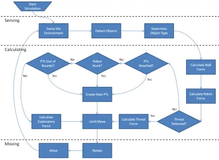
The robot achieves motion with three basic modes of operation. These include sensing

the environment, calculation of next step, and moving towards the next location (executing

the step) as seen in Figure 3.1.

3.2.1

Movement - Sensing Mode

In the sensing mode, the robot will use the omni-directional range finders to detect the

distance to any surrounding objects. Identifying if an object is a friend-or-foe (IFF) is not a

trivial task. There has been ongoing long-term research into this area [3] and in accounting

(28)

[image:28.612.92.525.225.542.2]

(29)

robot will know the type of object when it has sensed it. In actuality, the IFF could be

achieved in low cost robots with cameras by sensing the color or the shape of the object.

Other more extensive solutions may involve attempting to communicate with the object

using RF (Radio Frequency) communication. After the robot determines where the objects

are and what type they are, the next step is to use this information to determine the robot’s

movement, described in Section 3.2.2.

3.2.2

Movement - Calculation Mode

The most complicated and important mode of the robot operation is the second mode, the

calculation mode. The robot uses the distance from each of the objects to determine the

forces exerted on the robot. The calculation mode fuses several approaches to determine

forces needed to establish the next move, including Artificial Potential Fields, protecting

against the Local Minima Problem, collision avoidance, and threat handoff.

Artificial Potential Fields

Artificial Potential Fields (APFs) are a simple and low overhead method commonly used for

path planning. The APFs are also used for other robot formation[12, 15] and surveillance[8]

as described earlier.

The basic principle of the Artificial Potential Field is a system of forces all acting

to-gether on object moving through an environment. Several forces can be potentially

com-bined in a unique way to help solve this scenario. This APF will achieve the objectives

of the algorithm with simple calculations that are trivial for the robot to calculate with its

limited hardware. Along with the forces, the robot will makes decisions as to which forces

to ignore to better help to achieve the goal and protect the area.

The forces include the following (Figure 3.2):

1. Threat to Robot Force

(30)

[image:30.612.141.480.120.641.2]

(31)

3. Wall to Robot Force

4. Exploratory Force

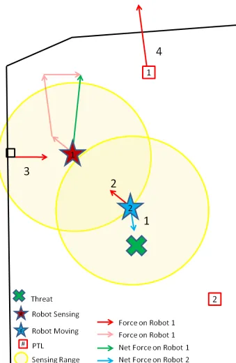
Figure 3.2 shows the interaction of all the forces that effect the robot’s movement. In

the diagram the red star is robot 1. The diagram shows robot 1 in the process of sensing

it’s environment and may be in either the sensing or moving mode of operation. The blue

star is robot 2 which is actively moving in the step that it has previously calculated. The

yellow circles around the stars show the effective sensing ranges of the robots. The green

X is a threat that robot 2 was affected by when it calculated its next move. The net forces

on robot 2 are shown with the blue line. The black line is a wall or boundary of the

surveillance region, and the red squares are the patrol target locations for robots 1 and 2

(labeled). Finally, the red lines are forces acting on robot 1. The faded red lines are the

projected forces on robot 1, and when placed end to end forms the green line for the net

force on robot 1. Robot 1 has the robot, wall, and exploratory forces acting upon it to make

this net force. The direction of the robot’s move will be in this direction. The robot’s step

will be calculated based on the combination of these forces, and later limited by several

factors.

The artificial potential field is essentially an area with differences in potential that form

hills and valleys. The valleys of the region apply forces on the robots similarly to a ball

rolling down a hill. The robot will move towards the areas with lowest potential. The patrol

target locations (PTLs) are the locations of lowest potential, and a wall or other robot is at

a point with the highest potential[20]. The quadratic APFs used in this research build upon

those used in [8]. All four of the forces are implementations of these quadratic APFs.

Below is the simple equation for the force with respect to the potential. The details of

calculating an actual move based on the force will be discussed at the end of this section.

− →

F =−_O−→P

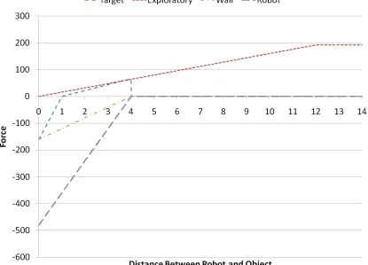
The Threat to Robot force is a two part attractive and repelling force. When the threat

(32)

threats are within the robot’s sensing range, the closest threat will be eliminated first. The

force toward the threat on the robot is larger the farther the robot is from the threat. This

force pulls on the robot until it is within the ideal distance from the threat. When this occurs,

the force will reverse direction and push the robot away from the threat. The ideal distance

used for simulation will be 1 meter. This essentially pushes and pulls the robot from the

threat until it settles at the ideal distance from the threat. After a predetermined amount of

time after the robot has detected the threat, this threat will be considered neutralized and

the robot will continue to seek other threats. During this time all, other forces are ignored.

[image:32.612.105.520.304.603.2]

This force can be seen in Figure 3.3.

Figure 3.3: Artificial Potential Field Forces

The Robot to Robot force is a repelling force that only acts upon the robots when they

(33)

krta = 11 Attracting Constant toward the

Threat.

krtr =−80 Repelling Constant away from the

Threat.

drt= 1 Optimal distance (threshold at

which the force flips).

Frt=

2krta|(x−drt)|, x > drt

2krtr|(x−drt)|, x <=drt

Table 3.1: Threat to Robot Force

robots come to each other. This effectively achieves a simple collision avoidance

mecha-nism. If the threat is also within the sensing range of the robots, the robot that is farther

away from the threat will ignore the Threat to Robot force and continue exploring the

surveillance region looking for other threats. This force can be seen in Figure 3.3.

srad = 4 The sensing radius of the robot

(limited by sensors).

krtr = 60 Repelling Constant away from the

Robot.

Frt= 2krtr(|x| − |srad|)

Table 3.2: Robot to Robot Force

The Wall to Robot force is a slightly more complicated repelling force. The robot will

be affected by the obstacle as soon as it is detected within its sensing range, similar to the

behavior of the other forces. However, it will not be a force acting in the direct angle to

the robot. Instead, the angle of the force will be α−90, whereαis the angle of incidence between robot and the obstacle. This ensures that the robot will travel in a more variable

direction to help keep the robot from traveling the exact same path continually. This force

can be seen in Figure 3.3.

The final and most complex force is the Exploratory force. This force keeps the robot

moving to new areas to explore instead of settling to a particular region. Several

com-ponents make up this force. A new point of interest is calculated based on the last several

positions that were used as points of interest. The points of interest are the locations that the

(34)

krtr = 8 Repelling Constant away from the

Wall.

Frt= 2krtr(|x| − |srad|)

Table 3.3: Wall to Robot Force

force from the last n points of interest (n is a variable calculated through experimentation)

with a time step assuming a constant speed (also a variable modified through

experimenta-tion). The robot does not move directly towards the point of interest. Instead, its move is

directed by a combination of the force towards the point of interest and one perpendicular

to it (Figure 3.4). The net force on the robot will cause it to spiral inwards toward the point

of interest thus covering more of the area while searching for threats. This spiraling force

is based upon the ladybug exploration force [18]. It is the secondary component of the set

of three algorithms. When the spiral angle is set to 0, the robot will move directly towards

the patrol target.

krta = 20 Attracting Constant effecting

movement toward the PTL.

Frt= 2krta(|x|)

Table 3.4: Exploratory Force

The force is not enough to determine how the robot actually moves. This must be

translated into an actual move. Using the force, the move can be calculated by finding the

velocity of the move over a time step. SinceF =m∗awhereais the acceleration, and we are assuming for simplicity that the mass (m) of the robot is 1, thenF = a. The velocity

v can be related to the acceleration via the equationv =a∗δtsubstituting in the force for acceleration to getv =F ∗δt. The final step to get the displacement or the move based on the force. Since disp=v ∗δt, thendisp =F ∗(δt)2. For simulation purposes a constant

δt= 0.15is used for a final formula ofdisp=F ∗0.0225.

(35)

[image:35.612.182.419.179.566.2]

(36)

closest robot and wall. These displacements will be added to the current location of the

robot. If there is a threat within the robot’s sensing range, the robot will calculate the

displacement based on the threat force, otherwise the exploratory force will be added

in-stead. The algorithm for the exploratory force involves a few more steps than the other

forces. These steps help to avoid a common problem with APFs called the Local Minimum

Problem.

Local Minimum Problem

Local minima can occur when the attractive and repulsive forces cancel out and effectively

trick the robot into thinking that it is at the PTL without being attracted in any direction.

The robot will stop moving and be locked or ”stuck” in a single location with little or no

movement. This can commonly occur when the robot is close to walls (especially corners)

or when the robot is close to other robots. Several approaches exist to overcome this

phe-nomenon. Yagnik et al.overcame the local minima problem in their research work with

a hybrid APF approach with simulated annealing[21]. Simulated annealing replaces each

step of the current solution with a random ”nearby” solution. This approach yields a good

solution even in the presence of noisy data, but may not be the most optimal due to

neigh-bors being chosen randomly. A more exhaustive search may yield better results, but could

take more processing time.

The local minima problem has been overcome in the surveillance algorithm in this

research by keeping track of the number of moves or steps that the robot makes since the

last PTL had been created. If number of steps is larger than a simple threshold, then the

robot must be in a local minimum. The threshold used for simulation is based on the PTL

distance and a constant.

Msm = 1.1 Max Step Multiplier.

Gdist PTL Distance.

Sthresh=d(Gdist∗Msm)e Step Threshold

(37)

When this scenario is detected of being ”stuck” in a local minimum, the robot

imme-diately calculates a new patrol target location. The final determination the robot makes

after trying to reach the PTL is whether the robot cannot reach the PTL because it is out

of bounds. When the robot senses the wall, it sees a line. The robot can easily establish

the orientation of this line based on the angles of the end points of the wall to the angle

the PTL is from the robot’s current position. If the PTL is determined to be out of bounds

the robot creates a new PTL in this scenario as well. The exploratory force displacement

is now calculated if no PTL was created. This displacement is added to the robot’s current

position. The next step for the robot is to now determine whether it is safe to make the

move that it has just calculated.

Collision Avoidance

The artificial potential fields create the individual move that the robot creates and moves

along when in the movement mode. The sum of all forces creates the raw move. Since the

robot does not actively sense the environment while moving, only sensing and detecting

when in the sensing mode, the robot must have some way to keep from colliding with other

objects. The collision avoidance method is a simple limitation of the calculated raw move.

All objects need to be avoided, including walls, threats, and other robots. Limitations

are put on the distance of the move in order to keep from colliding with each. When a

threat is detected, the robot limits itself to a move no larger than the distance to the threat.

Since the magnitude of the threat force will overwhelm any other forces and the exploratory

force will not be in effect, the robot will not collide with the threat. In order to keep from

colliding with other robots, the robot limits the move to1/2the sensing range of the robot. This is further limited to 1/2the distance to the closest robot if a robot is within sensing range.

The robot will also limit the move for the step to1/2the distance to the closest wall within sensing range. The limit is less than the distance to that closest wall to keep the

(38)

a small move, it becomes difficult for the robot to move away from the wall. Extra moves

are necessary for the robot to break free.

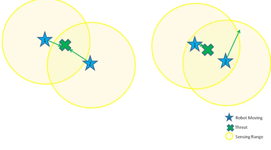
Threat Hand Off

There is no explicit hand off of threats between robots since the threats do not move. The

scenario does occur, however, where the threat may be identified by two separate robots.

One robot is assumed to be enough to eliminate a threat so the second robot would be

available to look for other threats. The hand off occurs with the following steps as shown

in Figure 3.5. When robot 2 detects the threat within it’s sensing range, it will move towards

the threat. When robot 2 senses robot 1 within its sensing range, it determines which robot

is closer to the threat. Robot 1 will do the same thing. The robot that decides it is further

away from the threat will ignore the threat and continue on with its move. Robot 1 was the

first to detect the threat and moved in closer to the threat before robot 2 had a chance to.

[image:38.612.91.525.406.647.2]

Therefore, robot 1 will be the closer robot to the threat and will neutralize it.

(39)

3.2.3

Movement - Moving Mode

The third mode of operation is movement. The robot turns in the direction of the calculated

movement and continues in that direction until it reaches the distance calculated for the

move. Individual moves will be created and traveled until the PTL is reached. If the PTL

cannot be reached due to the prior criteria (section 3.2.2), a new PTL will be created for

the robot to move towards. By this method, the robot is constantly moving, increasing the

area that is covered by the limited number of robots in the surveillance region.

3.2.4

Patrol Target Creation

The most novel feature of the three patrolling algorithms is the patrol target creation by

using robot sensing history. There are three different types of historic events that the robots

store in memory. While the robot is actively moving around the surveillance region, it

stores these points of interest as it comes across them. The historical points of interested

are listed in Table 3.6;

Historical Point Type Number Stored

Walls 2

Robots 1

Patrol Targets 1

Table 3.6: Historical Point Types and Number Stored

The robot keeps track of the last two walls that have been detected. When the robot

senses a wall, it first determines if a point close to the new wall point has already been

stored. It is not as useful to have two reference points for the same wall that are right

next to each other. It iterates through the array of wall locations stored finding any that

are within a threshold in distance from the current point that the robot is trying to store.

The threshold used for simulation is the sensing radius of the robot. This ensures that two

points near each other on the same wall will not both be stored for target generation. When

(40)

middle of the detected line segment representing the wall is stored. This makes for simpler

calculations and comparison of the walls.

For robot location history, only the last robot detected will be stored. If other robots

throughout the surveillance region were stored as well, there may be more cases where

local minima could occur. As the robot senses its environment and detects a new robot, the

previously stored robot is replaced by this newly detected robot. This may in fact be the

same robot, just at a different position than it was previously known to be located at.

Similar to the method of recording the robot historical point, only the last patrol target

location is stored and will be used. However, the storage of the patrol targets does differ

in two respects. First, when a new patrol target is created, it is not immediately stored in

the robot memory in the historical points. Instead, the point is stored in a general

infor-mation area for the robot that will guide each step as it moves towards the patrol target.

When the patrol target is reached, it is stored in a temporary location while a new patrol

target is generated. This previous target that was stored temporarily is now prepared to be

placed into the historical points memory and will be used on the next calculation to create

a patrol target. The preparation of the point involves storing a point half way between the

target and where the robot actually reached, instead of actually storing this exact target into

the memory. Due to local minima problems and the target actually being out side of the

surveillance region in many cases, it is not accurate to store the target directly. Through

experimentation it was also determined that it was best to store the PTL at this location

(subsection 5.2.2).

Testing was completed to compare the performance between three different methods of

storing the target (storing the target point where it was, where the robot was able to reach

before getting ”stuck” or determining the PTL was out of bounds, or halfway between the

points. It was determined that the point half way between the target and the robot’s end

point yielded the best performance in normalized time to detect targets (see Section 5.1 for

details on the performance metric). The next sections describe the process of establishing

(41)

flavors.

Initial Patrol Target

At the initiation of a simulation, there are no historical locations stored of any type.

There-fore, the robot must create a new patrol target with no history. A random angle from the

random robot start location is generated. The first patrol target is created at a distance ofdpt

from the robot start location at this initial random angle. The patrol target location distance

(dpt) is defined by table 3.7.

srad = 4 Sensing radius of the robot (limited

by sensors).

dpt=srad∗3 Patrol target location distance.

dpt= 4∗3 = 12 Final value of the constant patrol

target location distance.

Table 3.7: Patrol Target Distance

The patrol target distance is defined by the sensing range of the robot (4 meters)

multi-plied by a constant. During initial experimentation and algorithm creation, the best constant

was determined to be 3. This gives the robot a large swinging radius while spiraling towards

the PTL in the average target region of 60 meters by 60 meters square. A larger constant

will cause fewer patrol target locations while the robot is traveling across the surveillance

region which will ultimately cause a smaller region to be explored during a single pass

across the surveillance region. The possibility of basing the patrol target distance off of

the region size was explored initially. This was however, ultimately abandoned due to the

knowledge of the region that is necessary yet unknown to the robots.

Patrol Target Creation Scenario

The following scenario is an example of the calculation of a new patrol target based on

two wall history points and one PTL history point. For this simulation, no robot has yet

(42)

the initial configuration of the robot. The blue star is the robot and the yellow circle is the

sensing radius of the robot. The pink points are the historical points of interest, and the red

square is established as the new patrol target location. The pink lines connecting the robot

to the historical locations are merely for reference of the angle between the robot and these

[image:42.612.223.516.200.620.2]

locations.

Figure 3.6: Patrol Target Creation Step 1

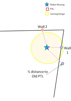
The robot first finds the angle to the first wall point (Wall 1 in Figure 3.7). It then

(43)

this wall point and adding 180◦. This now gives the direction of the new point. The distance

of the point is calculated to be at a constant distance from the robot’s current location (dpt,

Table 3.7). This new point is illustrated in 3.7 with a connecting blue line.

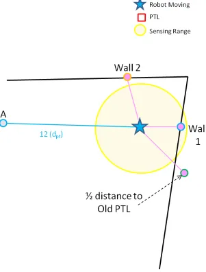
Next, the robot uses the second wall point in its patrol target location creation. It creates

a similar temporary point for reference from the robot at the opposite angle (180◦) from this

second wall point to the robot. This corresponding point and line are shown in Figure 3.8 in

[image:43.612.212.513.172.568.2]

(44)

the first temporary point A at that same opposing angle determined from the wall point 2

to the robot’s current location. A line representing the connection of temporary point A to

[image:44.612.213.516.216.567.2]

point B is shown in Figure 3.8.

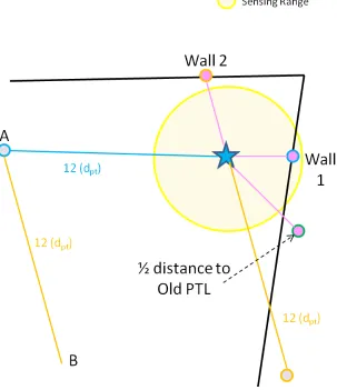
The new PTL can now be generated based on the final history point. The1/2distance to old patrol target has a similar temporary point to the wall points created at an opposing

angle from the robot again atdptfrom the robot’s current location. This same distance and

(45)

in the Figure 3.9 as a red box. A reference line in green has been drawn on the figure for

[image:45.612.105.516.142.554.2]

easy visualization.

Fading Effect

In an attempt to optimize the history algorithm a feature was added to fade the effect of the

robot and wall historical points over time. Three functions were tested on thedpt with the

(46)

dpt= 12 Patrol target location distance.

tcur Current simulated time (sec).

thp Time history point was first detected

(sec).

th =tcur−thp Time since the history location was first

identified (sec).

tf = 600 Time over which the history location will

fade away (sec).

cf = ((dpt/0.01)(1/tf))−1 History point fade constant.

dptlin =dpt−(dpt∗(th/tf)) Patrol target distance after linearly

de-creasing effect.

dptsf =dpt−(0.01∗((1 +cf)th)) Patrol target distance after slower fading

effect.

Table 3.8: Fading Patrol Target Distance

The linear function is a standard functions for linear decay. The slowly fading function

was derived to obtain the desired fading effect. Figure 3.10 shows the effect on thedptwith

these two functions and with no fading. The historical point fade time (tf) is a constant

used for every simulation. In the case of the two fading algorithms, the historical point will

have no effect on the patrol target generation at a simulated timetf after the time that the

point was first stored in the robot’s memory (thp). The effect of the fading historical points

is to further reduce the occurrences of local minima when the robot is moving through the

surveillance region.

Through experimentation it was determined that the optimal fading method for the

his-torical location of the previously seen robots was to have them fade linearly (subsection

5.2.1). There was an improvement on average but was not large enough comparatively

with the slowly fading method to warrant the more complex calculations that would tax

the processing capabilities of such a low cost platform. However, for the wall locations in

the history, it was also determined through experimentation that having the location of the

walls fade over time had a detrimental effect on the abilities of the algorithms. Since there

was no improvement, no fading was applied to the wall history locations for simulations

(47)

PTL history has no fading applied since the locations are replaced frequently (on every

[image:47.612.105.515.149.459.2]

calculation of the patrol target location).

Figure 3.10: Fading Effect of Historical Point

Random Path Patrolling

Using the robot’s sensing history is the primary component of two of the three algorithms

that were tested in this thesis. The first is the history with 45◦ maneuvering towards target,

and the second is the history with straight movement towards target, as enumerated in

section 3.2. One of the three algorithms tested, the Random Path Patrolling , however, does

not use this. It uses a much simpler method of patrol target generation called random path

(48)

Random path patrolling is an example of a random direction algorithm. For this

algo-rithm, the initial direction is created in the same method as the history algorithm. The robot

will travel in a straight line at this angle until it reaches a wall. When the wall is reached, a

new random angle is once again created. The angle is generated to be anywhere between 0◦

and 360◦from the robot’s current location (any direction in a circle). Because of this wide

window, it is possible and highly likely that the new angle will bring the robot towards the

wall again. The will cause a minimal amount of flutter as the robot is pushed in and out

from the wall (wall force and exploratory force opposing each other) until a new angle is

generated that points away from the wall. This is possibly not a very optimal method of

generating the random angle, and would be a good place for future improvement.

3.3

Memory Usage Analysis

One of the primary goals of this thesis research is to create an algorithm that simple low

cost robots are capable of supporting. The memory usage is a critical issue when the goal

is to run on a robot driven by a simple microcontroller with very little memory. Table

3.9 provides a high-level classification of the memory that will be needed by the robot to

complete any calculations for the history algorithms described in section 3.2.

Memory is needed for keeping the historical points as well as calculating new PTLs.

It is also used for various miscellaneous locations and timestamps. In addition, a section

of memory (48 32-bit floating point integers) is allocated for various calculations in the

algorithms. The calculated total memory needed is only 300 bytes. This is easily achieved

with the basic memory limitations of cheap microcontrollers found in many low cost robot

(49)

Number of Values

(32-bit floating point integers) Locations

2 History: PTL

4 History: Walls

2 History: Robot

2 PTL Creation: PTL

4 PTL Creation: Walls

2 PTL Creation: Robot

2 Misc: Current Robot Location

2 Misc: PTL Robot is Moving Towards

2 Misc: Temporary PTL Location

2 Misc: Sensed Threat

Number of Values

(32-bit floating point integers) Timestamps

1 Current Time

1 Time Robot Sensed (Fading)

1 Time Threat Sensed

Number of Values

(32-bit floating point integers) Miscellaneous

48 Enough for temporary values while

per-forming various calculations.

Total

[image:49.612.126.500.187.588.2]

24 + 3 + 48 = 75 75∗32bits= 2400bits= 300bytes

(50)

Chapter 4

Simulation Architecture

Simulation of the surveillance region has been completed using MATLAB for the

simula-tion environment.

4.1

Event Queue

An event queue model of simulation was chosen for implementation in the simulator for

the three surveillance algorithms. The event queue has the benefit of not requiring constant

time simulation and not requiring multi-threaded simulation where a thread of operation

is tied to each of the elements being simulated (the robots and threats in this case). The

simulator using an event queue was able to place the simulation events into a simple queue

that are operated on in order of time to be executed. All of the events in this simulation

occur when the robots were in their sensing and calculating modes. The first robot is

popped off the head of the queue and the algorithm of choice from the three described in

section 3.2 is run on it to determine the robot’s next move and if a new patrol target needs

to be created. When all calculations are complete, the robot is added back into the queue

sorted by time at which the robot should next enter its sensing and calculating modes.

This simple operation repeats until the simulation is completed. This simulation method

allowed for easy integration with the surveillance algorithms due to the robots only sensing

the environment while in the appropriate sensing mode and not while moving.

(51)

where the robots move separately and independently from each other. This is necessary

for the needs of this work because the robots must be completely autonomous. A discrete

simulation mode was briefly considered due to its simplicity, but requiring all of the robots

to be in the same mode of operation at the same time fell outside the parameters for desired

simulation. Each move would have had to have been exactly the same length and therefore

would have taken the same amount of time for travel, or enough simulated time would

have been given before the next sensing event for each robot to get to their destination.

This would be extremely inefficient in real-time with robots pending action and waiting for

others to finish.

4.2

Threat Arrival

The number of threats that will arrive in a given simulation run is provided as a parameter to

the simulator. The time at which they will start to arrive is a constant defined in the code as

600 seconds. The robots will arrive any time after the 600 simulated seconds (10 minutes)

have passed, but before 1400 seconds (23 minutes 20 seconds) have passed. When the

simulation starts the threats are placed in an array with a randomly generated start location

and a randomly generated arrival time between 600 and 1400 seconds of the simulation.

During the simulation run, the robots are not able to detect the threats unless the simulated

running clock is after the time at which the robot is slotted to appear.

4.3

Parameters

The simulator takes several parameters to define how the experimentation will run. This

section gives a brief overview of all of the important parameters to the simulator. Table 4.1

gives and example of each of these.

(52)

Parameter Value Explanation

simulationM ethod 0 Use robot history.

regionSize 60 Surveillance region is 60m square.

regionShape 1 Slightly irregular shape surveillance region.

numLoops 100 The simulator will run 100 simulations.

numRobots 2 Two robots actively patrolling the region.

numT argets 2 Two randomly appearing threats.

rotateAngle 45 45◦spiral towards patrol target.

numLocsGoal 1 Simulate storing one PTL location used for PTL creation.

rF adeT ime 600 Robots fade over 600 seconds.

rF adeM ode 1 Robots will fade from history linearly.

wF adeT ime 600 Walls fade over 600 seconds.

wF adeM ode 0 Walls will not fade from history.

[image:52.612.114.506.88.311.2]

storeP T LM ethod 3 Patrol target is stored1/2distance from robot. Table 4.1: Experiment Parameters

patrol target creation. For later experimentation, a value of 2 for the simulationM ethod

will run the simulations with a systematic walk method for a baseline comparison

(subsec-tion 5.3.6). TheregionSize parameter defines the general dimensions of the surveillance region over which the surveillance region shape will be overlaid. It is a single number

in meters that will be used to create a square region with each side being the value

pro-vided. The regionShapewill be one of the following shapes: 1 is for slightly irregular shaped region, 2 is for simple square shape, and 3 is for the highly irregular difficult shape.

The shapes will be discussed in more detail with the test of the algorithm for the

differ-ent shapes. It is easy to set the number test runs the simulator will run over the given

parameters, thenumLoopsparameter defines this.

ThenumRobots defines how many robots will be available to patrol the region. The

numT argets defines the number of targets that will appear over the lifetime of a single simulation run. TherotateAngleis the second critical piece of the algorithm configuration. If the simulationM ethodvariable is set to 0 the robot will use sensing history and the

rotateAngle will effect how the robot moves towards the patrol target. Both 45◦ and 0◦

(53)

PTLs that will be stored and later used for calculating new Patrol Target Locations. For

most experimentation only one PTL is stored (subsection 5.3.5).

The fade time parameters includingrF adeT ime andwF adeT imecorrespond to the

time over which the robots and walls will fade into having a smaller effect on patrol target

creation respectively. The parameters paired with theserF adeM odeandwF adeM odefor the robots and walls respectively correspond to the method by which the historic events

will fade into oblivion. Mode 0 means that the location will not fade, mode 1 means that

the location will fade linearly, and mode 2 means that the location will fade exponentially.

The final parameter storeP T LM ethod was varied during initial experimentation to find the optimal method of PTL storage for patrol target creation. A value of 1 corresponds to

storing the current location of the robot, 2 corresponds to storing the patrol target location,

and a value of 3 will cause the simulator to store the point half way between the robot’s

current location and the patrol target.

4.4

Simulation Visualization

As shown in the plot (4.1), the robots are represented by the different colored *’s and the

threats are represented by green X’s. When a threat is neutralized by a robot it turns into

a black X. Each robot has a number near it that represents the robot number assigned to

the robot for simulation and tracking. This number will not change during the simulation.

The yellow circle shows the omni-directional sensing range of each of the robots, and the

green line represents the path that the robot is following with this calculated move. A

red * (robot) is the current sensing robot. When it has completes sensing the region and

calculates its next move, it will become yellow. A yellow * (robot) represents one that is

turning towards the direction that it will be traveling in. Finally, a blue * (robot) shows that

the robot is moving along its calculated path. It will not sense the environment again until

(54)

[image:54.612.107.505.183.579.2]

(55)

A red square with a number inside is the current patrol target for the robot whose

num-ber matches that within the square. The historical point locations are represented by pink.

A pink #W# is for a wall history point for a robot represented by the #. A pink #R# is for

a robot history point for the robot represented by the #. And finally, a pink #G# is for a

previous patrol target (goal) for numbered robot.

As shown with the different colored robot symbols in the plot, there are several

real-world factors taken into account. First, the time for the robot to turn is factored into the

time for the robot to take its move and plot its turn. Second, a surveillance region that is

not a normal square shape is also used to test the ability of the algorithm to function in a

(56)

Chapter 5

Simulation Results and Discussion

5.1

Metrics

The primary goal of the algorithms developed is to eliminate threats when they appear in

the surveillance region as quickly as possible. One critical assumption is that only one

robot is needed to eliminate a threat. Therefore, the natural metric of choice for this type

of algorithm is the time it takes for the threat to be first detected after it appears. It is

not necessary to take into account the amount of time the robot will take to neutralize the

threat since this is a constant that will not change. In fact, the robots will stay locked into

the threat so it will take exactly the same amount of time to eliminate a threat every time.

The simulation keeps track of the arrival and first detection time of every threat within the

surveillance region, so that the time to eliminate the threat can be calculated.

The time that it takes to reach a threat is highly variable by nature. It is based on

where the robots are located at the time of the first appearance of the threats in the region.

Therefore, i

Autonomous robot patrolling of a sparsely populated unknown environment

Rochester Institute of Technology

Autonomous Robot Patrolling of a Sparsely Populated

Thesis Release Permission Form

Acknowledgments

Contents

List of Figures

List of Tables

Chapter 1

Problem Statement

Scenario

Technical Issues

Robot Limitations

Environment and Threat Arrival

Contribution

Robotic Platforms

Path Planning

Artificial Potential Fields

Preplanned Routes

Dynamic Routes

Chapter 3

Surveillance Algorithms

Movement - Sensing Mode

Movement - Calculation Mode

Movement - Moving Mode

Patrol Target Creation

Memory Usage Analysis

Chapter 4

Threat Arrival

Parameters

Simulation Visualization

Chapter 5