COMMUNICABILITY DISTANCE FUNCTIONS
ERNESTO ESTRADA† AND FRANCESCA ARRIGO‡
Abstract. We propose a communication-driven mechanism for predicting triadic closure in complex networks. It is mathematically formulated on the basis of communicability distance func-tions that account for the quality of communication between nodes in the network. We study 25 real-world networks and show that the proposed method predicts correctly 20% of triadic closures in these networks, in contrast to the 7.6% predicted by a random mechanism. We also show that the communication-driven method outperforms the random mechanism in explaining the clustering coefficient, average path length, and average communicability. The new method also displays some interesting features with regards to optimizing communication in networks.
Key words. network analysis; triangles; triadic closure; communicability distance; adjacency matrix; matrix functions;.
AMS subject classifications. 05C50, 15A16, 91D30, 05C82, 05C12.
1. Introduction. Complex networks are ubiquitous in many real-world scenar-ios, ranging from the biomolecular—those representing gene transcription, protein interactions, and metabolic reactions—to the social and infrastructural organization of modern society [12, 16, 44]. Mathematically, these networks are represented by graphs, where the nodes represent the entities of the system and the edges represent the “relations” among those entities. The accumulation of a mountain of empirical ev-idence has left little doubt that in general real-world networks are very different from those based on the uniform modelG(n, p) in many structural and functional aspects [16]. In particular, it is well-documented that real-world networks are significantly more “clustered” than one would expect from the previously mentioned uniform model [44]. The degree of “clustering” is usually quantified in network theory through the use of theclustering coefficient(see [53]). This accounts for the ratio of the number of triangles to the number of open triads, i.e. subgraphs of the typei−j−k. The fact that triangles are abundant in real-world networks has long been appreciated—for example, in 1922 where Simmel [52] theorized that people with common friends are more likely to create friendships. This “friendship transitivity” definitively implies a social mechanism for triadic closure in social networks which may then be applied to explain the evolution of triangle closures [30]. This Simmelian principle of triadic closure due to friendship transitivity assumes that individuals can benefit from coop-erative relations, and this may induce individuals to choose new acquaintances from among their friends’ friends.
The high degree of transitivity is not a unique feature of social networks; indeed, it is a common characteristic of many other types of networks such as biomolecular, cellular, ecological, infrastructural, and technological (see [16] and references therein). It is natural to assume that analogous cooperative principles to the one proposed by Simmel for social networks could be applied to find mechanisms that explain triadic closure in these other types of networks. Although intuitive, this simple idea has some fundamental drawbacks. First, it is not always true that pairs of nodes benefit
2
Department of Mathematics and Statistics, University of Strathclyde, 26 Richmond Street, Glasgow G1 1XQ, U.K. ([email protected]).
3
Department of Science and High Technology, University of Insubria, Como 22100, Italy ([email protected]).
from cooperative relations, and therefore the Simmelian principle is useless in such situations. Secondly, it is evident that not every pair of nodes separated by two edges participates in a triangle in a real-world network. Thus, some kind of selective process has been taking place, closing some of the triads in a network and leaving many others open.
The goal of this paper is to propose a general mechanism to account for such selective process of triadic closure in networks. We propose a strategy for predict-ing triadic closure based on the idea that triadic closure is a communication-driven process. This paradigm is formulated on the basis of communicability distance func-tions that account for the quality of communication between pairs of nodes using a mechanism accounting for both local and long-range interactions. We start with an overview of related work. All the mathematical concepts we use are introduced in Section 3 in order to make the paper self-contained. Sections 4 and 5 are devoted to the introduction of the new method for predicting triadic closure. We finish with a presentation and discussion of the results.
2. Related Work. Triadic closure, loosely defined as the process in which an edge is added to a triad to form a triangle, has long been considered as a fundamental mechanism of social networks’ evolution. The theoretical basis of this mechanism is due to Simmel [52] and one of the pioneering studies to use this principle to predict triadic closure in social networks was published by Krackhardt and Handcock [30].
When considering undirected networks, the main focus of triadic closure models has been to create simple mechanisms that provide insight into how (social) networks grow and generate their main topological characteristics. A simple model of network growth based on triadic closure has been proposed by Bianconi et al. [5]. They show that the evolution of networks based on such simple mechanisms “naturally leads to the emergence of community structure, together with fat-tailed distributions of node degree and high clustering coefficients”. Similar results by Klimek and Thurner [27] suggest that triadic closure can be identified as one of the fundamental dynamical principles in social multiplex network formation. These two works use triadic closure mechanisms based on the random selection of the nodes which will be involved in the triangles.
In the case of directed graphs an exhaustive computational analysis was performed by Leskovec et al. [31]. They consider several strategies to model how a nodeuselects a nodev, two steps from it, to form a triangle. The basic strategy is for uto select randomly a nodev from all the nodes at distance two. An alternative strategy is to assume thatufirst selects a neighbor nodewaccording to some mechanism, and then
w selects a neighborv according to some (possibly different) mechanism. The edge (u, v) is then formed and the triangle△uwv is closed. The selection of a neighborw
foru(orv for w) has been carried out using the following techniques: (i) uniformly at random; (ii) proportional to degree of w raised to a power; (iii) proportional to the number of friends that uand w have in common; (iv) proportional to the time passed sincewlast created an edge raised to a power; (v) proportional to the product of the number of common friends ofuandwmultiplied by the last activity time, all raised to a power.
Network % correct triadic closure random-random best
Flickr 13.6 16.9
Delicious 11.7 18.2
Answers 6.8 16.4
[image:3.612.198.403.93.163.2]Linkedin 16.0 21.4
Table 1
Illustration of the percentage of correct prediction of triadic closure in online social networks by the random-random selection of nodes and the best of all predictions made by Leskovec et al. [31].
which is undirected.
In a more recent paper, Lou et al. [32] have developed a method that adds so-ciological information to the network structure in order to predict triadic closure in a Twitter network. Their approach uses information about (i) geographic distance, i.e. whether users have a higher probability of following each other when they are located in the same region; (ii) homophily, i.e. whether similar users tend to follow each other; (iii) implicit network, i.e. how the following network on Twitter corre-lates with other implicit networks, such as the retweet and reply network; (iv) social balance, i.e. whether the reciprocal relationship network on Twitter satisfies social balance theory and to what extent. When this non-topological information is added, the developed method outperforms other structure-only approaches in the prediction of triadic closures. A similar approach, which uses demographic information instead, has been developed by Huang et al. [24]. They have used a large microblogging net-work as the source of their study, which reveals how user demographics and netnet-work topology influence the process of triadic closure. Their experimental results on the microblogging data show the efficiency of the proposed model for the prediction of triadic closure formation.
Here we will not account for extra-topological information, i.e., information apart from that provided by the topological structure of the network. Thus, our current work is more in the spirit of that of Leskovec et al. [31] with the difference that the networks we study are undirected.
3. Mathematical Preliminaries. A graph Γ = (V, E) is defined by a set ofn
nodes (vertices) V and a set of m edges E = {(u, v)|u, v ∈ V} between the nodes. An edge is said to be incident to a vertex uif there exists a node v 6=usuch that either (u, v) ∈ E or (v, u) ∈ E. The degree of a vertex u, denoted by du, is the
number of edges incident tou in Γ. The graph is said to beundirected if the edges are formed by unordered pairs of vertices. Awalk of length k in Γ is a set of nodes
u1, u2, . . . , uk, uk+1 such that for all 1 ≤ l ≤k, (ul, ul+1) ∈ E. A closed walk is a
walk for which u1 =uk+1. A path is a walk with no repeated nodes. A closed walk
of length 3 is called a triangle. We will calltriad every triplet of nodesu, v, andw
such that (u, v),(v, w)∈ E but (u, w)6∈E. Hence a triad is a triangle missing one edge. We shall call this missing edge apotential edge. A graph isconnected if there is a path joininguandv for everyu, v∈V. A graph with unweighted edges, no edges from a node to itself, and no multiple edges is said to besimple.
LetA= (auv)∈Rn×n be theadjacency matrix of the graph. It is worth noting
(see [23]) and its entries are:
auv =
1 if (u, v)∈E
0 otherwise ∀u, v∈V.
It is possible to define several distance measures on networks. The most common is theshortest-path(orgeodesic)distancebetween two nodesu, v∈V, which is defined as the length of the shortest path connecting these nodes. We will write d(u, v) to denote the geodesic distance between u and v. and hence the average path length
[16, 44], the average of the shortest path distances in the graph, is given by
ℓ= 1 2m
X
u,v∈V
d(u, v).
Another useful measure for characterizing the structure of networks is the so-called
local clustering coefficient of a nodeu[53], which quantifies the degree of transitivity of local relations in a network and is defined as
Cu=
2tu du(du−1)
,
wheretuis the the number of triangles in which nodeuparticipates. Taking the mean
of these values asuvaries among all the nodes in Γ gives theclustering coefficient of the network,
C= 1
n n X
u=1 Cu.
An important quantity to be considered when studying communication processes in networks is thecommunicability function [14, 17, 15], which is defined as
Guv = eAuv=
∞
X
k=0 Ak
uv k! =
n X
k=1 eλkq
k(u)qk(v), ∀u, v∈V,
where A =QΛQT is the spectral decomposition of the adjacency matrix (see [23]),
with Λ a diagonal matrix containing the eigenvalues ofA and Q = [q1, . . . ,qn] an
orthogonal matrix containing the associated eigenvectors.
Communicability counts the total number of walks starting at nodeuand end-ing at node v, weighting their length by a factor k!1, thus considering shorter walks more influential than longer ones. TheGuu terms of the communicability function,
which are usually calledsubgraph centralities of the nodes, characterize the degree of participation of a node in all subgraphs of the network, giving more weight to the smallest ones. Here we will use theaverage communicability as a way to characterize the quality of the communication taking place in the network as a whole:
G= 1
n(n−1)
X
u6=v Guv
departing from a source node reaches its target (Guv), and how much information
de-parting from the node returns to it without ending at its destination (Guu). That is,
the quality of communication increases with the amount of information that departs from the originator and arrives at its destination, and decreases with the amount of information which is wasted due to the fact that the information returns to its source without being delivered to the target. In [18] thecommunicability distance is defined as
(3.1) ξuv =
p
Guu+Gvv−2Guv.
It is a Euclidean distance between the nodes u and v in Γ (see [18, 19]). From its definition, it is clear thatξuv characterizes the quality of the communication taking
place between nodesuandv.
4. Communicability Distances and Triad Closure. We start by considering the square of the communicability distance defined in (3.1) for a pair of nodesuvin a connected graph. This distance characterizes communication quality between nodes
uand v by assuming that the information departing from node utravels to node v
(and viceversa) by taking a series of one-hop steps between the nodes in any of the walks that connect them. From (3.1), it is clear that the smaller the value of ξ2
uv,
the better nodesuv are at exchanging information. The communicability distance is dependent oneA, whereA is the adjacency matrix of a simple graph. If we consider uand vsuch that auv= 1, then we are assuming that these two nodes are attracted
to each other. If instead we were to consider that these nodes repel each other, we would usee−A.
If the (squared) communicability distance between two pairs of nodesuvand pq
satisfies ξ2
uv < ξpq2 then we say that the attraction between the pair uv is stronger
than that of the pairpqin the corresponding network.
Now, consider a triad u, w, v, where (u, w) ∈ E, (w, v) ∈ E but (u, v) ∈/ E. Becauseauw= 1 andawv= 1 we can infer that there are attractive “forces” between uandwand betweenwandv. A simple metaphoric way to represent such attractive forces between pairs of nodes is to suppose that they have opposite charges which attract to each other. For instance, we can consider either of the following schemes for the previous example: u+−w−−v+, u−−w+−v−. Notice that considering a particle spin, as is usually done in sociophysical models of opinion dynamics, also works here as an appropriate metaphor (see for instance [51]). Observe that there are two types of interactions between the nodes uand v. First, due to the attractions betweenu and wand w and v, the node v ‘feels’ an attractive force from u, which is transmitted through the edges of the network. On the other hand, due to the fact that both uand v have the same charge, they experience some repulsion from each other, which takes place in a ‘through-space’ fashion (which we will clarify later). We can expect the link (u, v) to be created if the through-edge attractive force between the nodesuandv is larger than the through-space repulsive force between them.
electrostatic forces. These interactions are analogous to our through-space repulsion and we will refer to them as direct Long-Range Communicability (LRC). In a social network, TEC is present when information is transmitted from one individual to another in the network by using the social ties that define the edges of the graph. On the other hand, LRC is realized by the direct influence of an individual to another through any source of social signalling.
Note that although the shortest path distance between every pair of nodes in a triangle equals one, every pair of nodes in it is connected by a pair of adjacent edges through the third vertex. A natural way to account for all the pairs of nodes connected by pairs of adjacent edges is to consider the number of walks of length two between the pairs of nodes. We can then transform a graph accordingly. Let Γ = (V, E) be a simple and connected graph and let W2(Γ) = (V, E′) be the graph with the same
set of nodes as Γ but whose edges are weighted by the number of walks of length two between every pair of (not necessarily distinct) nodes in Γ. More precisely, ifµ2(u, v)
is the number of walks of length two between nodesiandj, then the adjacency matrix ˜
AofW2(Γ) is
(˜a)uv =
µ2(u, v) u6=v µ2(u, u) =du u=v.
Remark 1. Clearly A˜ = A2 and so we do not need to explicitly construct the graph W2(Γ), since we can simply work with the square of the adjacency matrix of the graphΓ.
Note that two nodes are connected inW2(Γ) if they have the same charge and so
connected nodes inW2(Γ) repel each other. Consequently the repulsive
communica-bility between a given pair of nodes in Γ is given by ˜Guv= (e− ˜ A)
uv= (e−A 2
)uv.
A communicability distance based on ˜Guvaccounts for the quality of LRC between
pairs of nodes separated by two adjacent edges, i.e., pairs of nodes feeling mutual repulsion in Γ. We can define a communicability distance function by
(4.1) ηuv=
q
˜
Guu+ ˜Gvv−2 ˜Guv
A large value of ηuv indicates that there is a weak repulsion between nodes u and v. The proof thatηuv is a Euclidean distance between the nodesuandvfollows the
same lines as in [18, 19] and is omitted.
Remark 2. The graph W2(Γ) is not always connected and so the function ηuv is defined only for pairs of nodes which are in the same connected component of the graph. Elsewhereηuv is set to infinity.
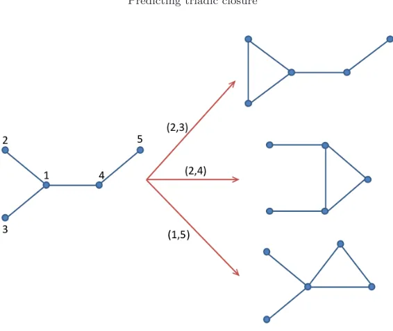
Before continuing, consider the following example. The tree illustrated on the left in Figure 1 can be transformed by adding an edge which closes any of the three nonequivalent existing triads of the graph, i.e. by adding the edge (2,3), (2,4) or (1,5). The resulting unicyclic graphs are illustrated on the right of Figure 1. In Table 4 we report the values ofξ2
uvandη2uvfor each of the three triads. Now assume that we have
information indicating that the process giving rise to the closure of the 1,2,3-triad is favored over the other two. We cannot knowna priori for any particular system how the attractive and repulsive forces scale. In real physical systems such terms are scaled by minimizing the global energy of the system. Here we simply consider the weighted difference between the two terms,αξ2
uv−βη2uv. We will propose a method to determine
the values of the empirical parameterαand β in a given network a little later. For this example it can be verified that, for instance, ξ2
Fig. 1.Example of evolution of a tree after one edge is added to close a triangle.
value only for the pair (2,3) (see Table 4). This weighted difference betweenξ2 uv and η2
uv corresponds to the case in which the attractive forces between the corresponding
nodes outweight the magnitude of the repulsive ones. As noted previously, a large value ofη2
uvindicates a small repulsion between the corresponding nodes, and here we
have multipliedη2
uv by a coefficientβ >1, which further reduces the repulsive forces.
Now suppose instead that we have information indicating that the process giving rise to the closure of the 1,4,5-triad is favored over the other two. In this case it can be verified (see Table 4) that the weighted difference−0.5ξ2
uv+ 1.5η2uvis negative only
for the pair (1,5). Here, we have considered that the attractive forces between the nodes make a negative contribution to the creation of an edge closing the triad. This may correspond to the situation in which the links (u, w) and (w, v) are both very weak, i.e. friendship ties between the corresponding individuals are not too strong. We further weaken those relations by multiplying ξ2
uv by a coefficient α < 0. At
the same time, by multiplying η2
uv by a coefficient β <0 we have assumed that the
repulsive factor does not play a major role in determining whether the new edge is created or not. Indeed, in this wayη2
uv is transformed into an attraction term. In the
charged-particles analogy this corresponds to a situation in which the charges between the corresponding nodes are very weak and there is no repulsion between those nodes separated by two adjacent edges.
Finally, suppose that we have information indicating that the process giving rise to the closure of the 1,2,4-triad is favored over the other two. In this case it can be verified (see Table 4) that the weighted difference ξ2
uv+ηuv2 reaches the smallest
value for (2,4). The values of the weighted differences for the three triad closure processes are positive, but the one corresponding to the closure of he 1,2,4-triad is the lowest among the three. In this case, triadic closure is dominated by attractive forces only. The termαξ2
uv withα >0 indicates the normal attractive forces between
the corresponding pair of nodes whileβη2
pair ξ2
uv η
2
uv ξ
2 uv−1.5η
2
uv −0.5ξ 2 uv+ 1.5η
2 uv ξ
2 uv+η
2 uv
2,3 2.000 2.000 -1.000 2.000 4.000
1,5 3.184 0.960 1.744 -0.152 4.144
2,4 2.545 1.312 0.577 0.696 3.857
Table 2
Values of weighted sum ofξ2
andη2
for the potential edges considered in Figure 1.
term.
A case we haven’t considered here is if α < 0 and β > 0, when both terms represent repulsive forces between nodes. In this caseαξ2
uv−βηuv2 <0 for allu, vand
the order in which the triads will be closed is determined by the magnitudes ofαand
β. In such a repulsive system there are no attractive forces to fuel the creation of new edges. Consequently, the creation of the new edges to close triads is controlled by factors such as their similarities or complementarity in their functions which do not depend particularly on the communicability between nodes. In this case, predictions of triad closure made on the basis of communicability distances are not expected to differ significantly from those made by a random closure of the triads.
In summary, we can use the function
(4.2) ∆uv(α, β) :=αξuv2 −βη 2
uv, ∀u, v∈V,
to determine which triad is closed in the network.
In order to predict which triads will close in a given network it is necessary to know the values ofα and β. We now propose a method that allows us to estimate these empirical parameters and consequently to determine which triads will close in a given network.
5. Proposed Method. In order to predict the triadic closure in a network based on ∆uv(α, β) we develop a procedure to find the values of the empirical parameters α and β which best predict the triadic closure in a network from which we have a priori removed all the triangles. That is, if we take a network Γ, we first detect all its existing triangles. We then transform Γ into a triangle-free graph Γ′ by removing one and only one of the edges forming each triangle. The deleted edges are selected uniformly at random from the three edges forming each triangle. As this procedure is likely to be repeated a large number of times (see below for details), the chance that each of the three edges is selected at least once is very high. We keep a list of all these removed edges which we callR. It may happen that two trianglesT1andT2
share an edgee. If we selectewhen consideringT1, then, when it comes to select an
edge inT2, we pick an edge which may or may not coincide withe. If it does, we do
not add it to the list. It may also happen thatT2consists of eand two other edges,
one of which has also already been removed because it was in common with a third triangle. In such cases, we do not remove the last connection remaining in T2, since
it could disconnect the network.
the triadic closure process should be controlled by the smallest values of ∆uv(α, β)
(see example in Figure 1). Thus, we expect that a non-increasing ranking of the values of ∆uv(α, β) contains most of the elements ofR at the top of the ranking and those
ofP at the bottom.
In order to quantify the percentage of triangles that were correctly predicted we proceed as follow. We first rank the entries ofL in non-increasing order. We select the toprentries of L=R∪P, wherer is the cardinality ofR. Then, we count the numberrp of entries in this toprwhich are elements ofR. These entries correspond
to those pairs of nodes which were originally part of the triangles of Γ. That is, rp
represents the number of correct predictions made by the current method. We call the (percentage) ratio ofrp to rthe percentage ofdetected.
5.1. Datasets and Computational methods. We now give some computa-tional details on how we implemented these calculations to find the optimal values of
αandβ for a selection of networks.
We study 25 networks representing complex systems from a wide variety of envi-ronments, such as social, ecological, biomolecular, technological, infrastructural, and informational. A brief description of all these networks is given in the Appendix.
In order to find the optimal values of the empirical parameters α and β for these networks we proceed as follows. We calculate all the values ofαand β in the intervalI= [−2.1,2.1] with a step length of 0.1. This intervalIhas been determined empirically as smaller intervals led to worse results and larger ones did not improve the results. Then, for each combination ofαandβ in ∆uv(α, β) we rank all the elements
ofLin non-increasing order and find the percentage ofdetected. The optimal values
ofαand β for this particular network are those that produce the highest percentage ofdetected. These computations were repeated 100 times.
The effectiveness of the proposed method is tested by considering a simple null model constructed as follows. We randomly order the edges inL, select the toprpairs of nodes and count how many of them were in the set R. With this information we compute the percentage of correct predictions made by a random ordering of the pairs of nodes (rand). Similar values of the percentages of detected and rand indicate
that the ranking produced by the function ∆uv(α, β) does not differ significantly
from a random ordering of the pairs of nodes and consequently is not a good one; while larger differences between the percentages of detectedandrand indicate good
performance of the proposed method.
Before starting with the detailed analysis of these 25 datasets we consider the possibility of fixing one of the parameters (α or β) and letting the other varying in the bounded interval [−2.1,2.1]. To do this we set α = 1 and let β vary. This seems reasonable, since this choice allows us to tune the disturbance caused by the repulsion in the values of ∆uv. However, the results obtained for 10 of the studied
networks discouraged us from proceeding with this approach. On average the use of the two parametersαandβ makes predictions of triadic closure which are 7% higher than those using only one parameter, with maximum differences of up to 20% for one network (results not shown here). Thus, we will use the more general approach of calibrating both empirical parameters.
5.2. Bounds for communicability distance functions. Although in our ex-periments we use the exact values of the communicability distance functions in order to obtain the values of ∆uv, we now give some bounds forξuv andηuv, which can be
be too costly to compute. To avoid the computation of the matrix exponential, we de-rive bounds forξ2
uvandη2uv(and therefore for ∆uv(α, β)) by means of a Gauss–Radau
quadrature rule. In order to make the present paper self-contained, we summarize the approach used as described in [2, 1, 21] before giving these bounds.
It is well known that the problem of computing bilinear expressions of the form uTf(A)vcan be reduced to the approximation of a Riemann–Stieltjes integral with
respect to a certain measure using quadrature rules. Indeed, in a series of papers, Golub and collaborators use 1 step of the symmetric Lanczos iteration to give bounds on the entries of f(A) based on Gauss-type quadrature rules when f is a strictly completely monotonic (s.c.m.) function on an intervalI containing the spectrum of
A. Recall that a function is s.c.m. on I if f(2k)(x) > 0 andf(2k+1)(x) < 0 for all x∈ I and ∀k≥0. Since g(x) =ex is not s.c.m., we need to work on f(x) =e−x to
derive bounds on the quantities of interest here.
The key result that allows to easily compute a priori bounds using Gauss-type quadrature rules is that we can use the element in position (1,1) of the matrixf(Jp+1)
(see Theorem 6.6 in [21]), where
Jp+1=
ω1 γ1 γ1 ω2 γ2
. .. ... ...
γp−1 ωp γp γp ωp+1
is a tridiagonal matrix whose eigenvalues are the nodes of the quadrature rule, and the rule’s weights are given by the squares of the first entries of Jp+1’s normalized
eigenvectors.
Our results are summarized in the following theorems.
Theorem 5.1. Let A be the adjacency matrix of an unweighted and undirected network. Then
(5.1) Φ
b, ω1+ γ 2 1 ω1−b
≤(ξuv)
2
2 ≤Φ
a, ω1+ γ 2 1 ω1−a
,
where
(5.2) Φ(x, y) =c(e
−x−e−y) +xe−y−ye−x
x−y , c=ω1,
(
ω1=auv,
γ1=du+d2 v −ω1−A2uv 12
,
and[a, b]is an interval containing the spectrum of −A.
Remark 3. If (u, v)6∈E the bounds simplify considerably. Indeed, in this case ω1= 0 and hence
b2eγ12
b +γ2
1e−b b2+γ2
1 ≤
(ξuv)2
2 ≤
a2eγ12
a +γ2
1e−a a2+γ2
Before proceeding with the proof of the result, note that (ξuv)2can be written as
(ξuv) 2
= (eu−ev)T eA
(eu−ev),
whereeu andev are theuth andvth vectors of the canonical basis, respectively. Proof. Using the Lagrange interpolation formula for the evaluation of matrix functions [22] one can easily show [1] that
eT1(e−C)e 1=
c11(e−µ1−e−µ2) +µ1e−µ2−µ2eµ1 µ1−µ2
.
whereµ1,µ2 are the distinct eigenvalues of the matrixC.
We now want to build explicitly the matrixJ2=
ω1 γ1 γ1 ω2
in such a way that
τ1 = a or τ1 = b is a prescribed eigenvalue. The values of ω1 and γ1 are derived
explicitly by applying one step of Lanczos iteration to the matrix−A with starting vectorsx−1=0andx0= (eu−ev)/
√ 2.
Note that ifγ1 = 0 we simply takeω2 =τ1 and the matrixJ2 is diagonal with
eigenvaluesµ1 =ω1 and µ2=τ1. Thus, let us assume γ1 6= 0. Using the three-term
recurrence for orthogonal polynomials:
γjpj(λ) = (λ−ωj)pj−1(λ)−γj−1pj−2(λ), j= 1,2, . . . , p,
withp−1(λ)≡0,p0(λ)≡1 we find thatω2=τ1−p1(τ1)γ1 . Using the same recurrence,
we also find thatp1(τ1) = (τ1−ω1)/γ16= 0, since the zeros of orthogonal polynomials
satisfying the three-term recurrence are distinct and lie in the interior ofI (see [21, Theorem 2.14]).
The matrix
J2=
ω1 γ1
γ1 τ1− γ 2 1 τ1−ω1
!
has (distinct) eigenvaluesµ1 =τ1 and µ2 =ω1+ γ 2 1
ω1−τ1. The result then follows by
applying Theorems 6.4 and 6.6 from [21]. Similar bounds can be computed forη2
uv and are described in the following
theo-rem, whose proof matches that of Theorem 5.1.
Theorem 5.2. Let A be the adjacency matrix of an unweighted and undirected network. Then
Φ
˜b,ω˜1+ ˜γ12
˜
ω1−˜b
≤(ηuv)
2
2 ≤Φ
˜
a,ω˜1+ γ˜ 2 1
˜
ω1−˜a
whereΦis defined as in equation (5.2) withc= ˜ω1,I˜= [˜a,˜b]is an interval containing the spectrum ofA2, and
˜
ω1=γ12+ω1;
˜
γ1= h
1 2
Pn
w=1 A2uw−A2wv 2
−ω˜12 i12 .
withω1 andγ1 as in theorem 5.1.
ofA. For these values, the bounds simplify to
Φ
a2,ω˜1+ ˜γ 2 1
˜
ω1−a2
≤(ηuv)
2
2 ≤Φ
0,ω˜1+˜γ 2 1
˜
ω1
= ω˜
2 1e
−ω˜
2 1+˜γ12
˜
ω1 + ˜γ2 1
˜
ω2 1+ ˜γ12
.
Combining the results described in the previous theorems, one easily get bounds for the values of ∆uv(γ,β)
2 . Indeed, the computation is straightforward, since the new
bounds are linear combinations of the previous ones. For example, if we haveγ≥0 andβ≤0 we get as lower bound for ∆uv(γ,β)
2
γΦ
b, ω1+
γ2 1 ω1−b
+βΦ
˜
a,ω˜1+
˜
γ2 1
˜
ω1−˜a
,
and as upper bound
γΦ
a, ω1+
γ2 1 ω1−a
+βΦ
˜
b,ω˜1+
˜
γ2 1
˜
ω1−˜b
,
whereω1,γ1, ˜ω1, and ˜γ1depend on the choice ofuandv.
6. Modeling Results and Discussion.
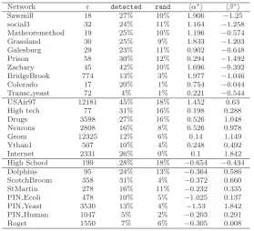
6.1. Predicting and interpreting triadic closure. The first series of results refers to the finding of the optimal values ofα and β for the studied networks and the comparison of the percentage of triadic closures correctly predicted by the pro-posed method in comparison with the random process. The results of the tests are listed in Table 3. The columnshα∗iandhβ∗icontain the average best values for the parameters, where the average is taken over the 100 iterations we run. The results show that on average the method based on the communicability distance functions (detect) correctly predicts 20% of the triad closures in the real-world networks
stud-ied. In 7 cases this percentage of correct prediction reaches values larger than 25%. In contrast, the random closure of triads identifies 7.6% of the real triangles existing in those networks.
We can now gain some insights about the processes that have governed the triad closure in the studied networks. Recall that in general the triadic closure process consists of two different means of transmission of information, namely the TEC and the LRC. If we refer to the nature of the two kinds of transmission in the order TEC-LRC we can have any of the following four scenarios:
closed by an attraction-repulsion mechanism. The only network with a repulsion-attraction triad closure mechanism is the social network of High School, while there are 7 networks closing triads with a repulsion-repulsion mechanism (three protein-protein interaction (PPIs) networks, two food webs, one animal social network and the Roget thesaurus).
The group of networks with attractive-attractive interactions consists of 63% of all the social networks studied here. Among them we find a communication network within a small enterprise: a sawmill, where all employees were asked to indicate the frequency with which they discussed work matters with each of their colleagues on a five-point scale ranging from less than once a week to several times a day. Two employ-ees were linked in the communication network if they rated their contact as a three or higher. This is a cooperative process in which both advisers and advisees cooperate to share the information needed for improving their skills and knowledge. Thus, closing the potential triangles in order to enhance the communication between the individuals involved seems a very reasonable mechanism. The other social networks included in this class all share a common characteristic. In the networks Social3 (a network of social contacts among college students participating in a leadership course), Gales-burg (a network of friendship among physicians) and Matheoremethod (a network of friendship among school superintendents) the participants in the respective studies were asked the following questions:
• Choose the three members they wished to include in a committee;
• Nominate three doctors with whom they would choose to discuss medical matters;
• Name their best friends among the chief school administrators in Allegheny County.
In the first two cases it is very clear that the participants were asked to nominate individuals with whom they would easily cooperate, e.g., members of a committee or colleagues with whom to discuss medical matters. The third resembles a general kind of friendship relation, but the question was formulated in the context of analyzing the diffusion of a new mathematical method among High Schools in the county. Thus, se-lecting your best friends among other chief school administrators also means sese-lecting those with whom you would easily cooperate in technical matters. These facts may explain the kind of attraction-attraction interaction which dictates the main mecha-nism for closing the triads in these networks. Transmission of information through the edges as well as a direct long-range interaction between peers both benefit the cooperative atmosphere needed for performing the tasks for which these networks are created.
In the class of networks in which triads have been closed by attraction-repulsion mechanisms we find networks of very different natures and it is difficult to extend the previous analysis to all these networks. This group includes a social network in a small high-tech computer firm which sells, installs, and maintains computer systems, where individuals were asked: “Who do you consider to be a personal friend?”. It could be speculated that a mechanism of the type based on Simmelian principles dominates here. That is, ifA−B−C is a triad and the two pairsA−B andB−Chave strong social relations, it is natural to think that there is not a strong repulsion betweenA
Table 3
Results of the proposed method for predicting triad closure in 25 complex networks.
Network r detected rand hα∗i hβ∗i
Sawmill 18 27% 10% 1.906 −1.25
social3 32 24% 11% 1.164 −1.258
Matheoremethod 19 25% 10% 1.196 −0.574
Grassland 30 25% 9% 1.833 −1.203
Galesburg 29 23% 11% 0.902 −0.648
Prison 58 30% 12% 0.294 −1.492
Zachary 45 42% 10% 1.696 −0.392
BridgeBrook 774 13% 3% 1.977 −1.046
Colorado 17 20% 1% 0.754 −0.044
Transc yeast 72 4% 1% 0.221 −0.544
USAir97 12181 45% 18% 1.452 0.63
High tech 77 31% 16% 0.198 0.288
Drugs 3598 27% 16% 0.526 1.048
Neurons 2808 16% 8% 0.526 0.978
Geom 12325 12% 6% 0.14 1.149
Ythan1 507 10% 4% 0.248 0.492
Internet 2331 26% 0% 0.1 1.842
High School 199 28% 18% −0.654 −0.434
Dolphins 95 24% 13% −0.364 0.586
ScotchBroom 358 31% 4% −0.372 0.660
StMartin 278 16% 11% −0.232 0.335
PIN Ecoli 478 10% 5% −1.025 0.137
PIN Yeast 3530 13% 4% −1.53 1.842
PIN Human 1047 5% 2% −0.203 0.291
Roget 1550 7% 6% −0.305 0.008
and B−C are not strong enough to tie A andC together. If the pairsA−B and
B−Chave some strong relation, i.e. if they are dating, a link betweenAandCcould be seen as offensive to the already established couples. The final class of networks, that characterized by repulsion-repulsion interactions, does not contain any human social network. The three PPIs included in this study are characterized by this type of triad closure mechanism, together with 2 food webs, an animal social network and a thesaurus. The repulsion-repulsion mechanism is characterized by weak through-edge transmission of information and weak long-range interaction between pairs of nodes separated by two adjacent edges. Thus, it is expected that the triad closure is controlled by non-topological factors, such as similarities or complimentarities among the nodes. This is a plausible explanation for the case of the PPI networks where triads of proteins may form triangles due to their functional similarities. We notice that, as expected, the percentages of correct prediction of triad closure in this group are the smallest of the four groups. That is, the difference between the predictions made by the proposed method and the random one in this group is 8.7%, in contrasts with 15.5% for the attraction-attraction, 14.1% for the attraction-repulsion and 10% for the only network with repulsion-attraction mechanisms.
network of injecting drug users (Drugs) for which we consider the clustering coefficient, the average path length, and the average communicability of the actual network. In order to perform these experiments we select 50% of the total number of triangles existing in the network and we remove one edge from each of them. Edges are selected uniformly at random among those present in the corresponding triangle. As before, letLbe the list of edges obtained from the union of the potential edges and of those we removed. The values for α∗ and β∗ are those determined empirically using the calibration method already described (cf. Table 3).
The iteration process goes as follows. We select the potential edge realizing the smallest value for ∆uv(α∗, β∗) and we add this edge to the network. Then we compute
the values of the parameters of interest: the average clustering coefficient, the average path length, and the average communicability. Finally, the values for ∆uv(α∗, β∗) are
recomputed using the new adjacency matrix, obtained by the addition of the selected potential edge. Here every addition of an edge is considered as a time step.
This iteration is run as many times as the number of edges we have removed. That is, if we removedr edges, we consider a discrete time evolution for 0≤t≤r. We then repeat this experiment 10 times, taking the average and standard deviations of the corresponding parameter. In order to compare the results we simulate the same process by adding such edges uniformly at random.
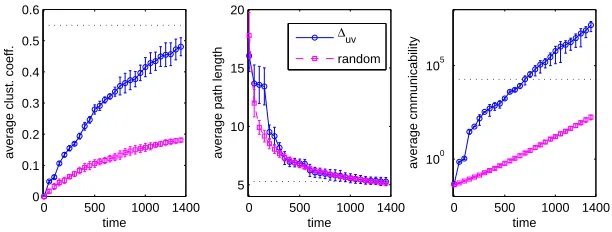
The results of this experiment are illustrated in Figure 2, where we plot the values for the parameters of interest (with the corresponding error bar) versus time. The horizontal dotted line represents the actual value of the property for the original real-world network. As can be seen in Figure 2, the proposed method outperforms the random one for predicting the clustering coefficient of the network. The current value ofC for this network is 0.549, while the one predicted by ∆uv is 0.486, which
contrasts with that of 0.183 obtained by the random method. We remark here that this is the most important parameter to be considered in this experiment as it is the one which accounts more directly for the ratio of triangles to paths of length two in the network. Both methods predict the average path length of the network very well, returning values very close to the actual one (ℓ = 5.287). In addition, the proposed method increases the average communicability of the network more significantly than the random triadic closure. This feature is important when one is interested in maximizing the total average communicability of a network, which is equivalent to increasing the quality of communication among the nodes in the network.
7. Conclusions. The prediction of triadic closure is a very important and far from trivial problem in network theory. The fact that most real-world complex net-works have more triangles than random counterparts makes the problem interesting
0 500 1000 1400 0
0.1 0.2 0.3 0.4 0.5 0.6
time
average clust. coeff.
0 500 1000 1400 5
10 15 20
time
average path length
0 500 1000 1400 100
105
time
average cmmunicability
∆uv
[image:16.612.157.463.114.230.2]random
Fig. 2.Illustration of the evolution of the clustering coefficient, average path length, and average communicability for the network of injecting drug users (Drugs) versus the number of links added
using the function (∆uv) and at random (see the text for explanations).
matrix representation of a multiplex the communicability function has been obtained and studied for social and technological multiplexes [13]. Consequently, the current approach can be extended to consider communicability distances among the nodes in multiplexes and in this way to apply the current methodology to detecting triadic closure in these structures.
Acknowledgements. E.E. thanks the Royal Society for a Wolfson Research Merit Award.
Appendix.
In this section we give a brief description of the networks used for the tests throughout the paper.
Brain networks
• Neurons: Neuronal synaptic network of the nematodeC. elegans. Includes all data except muscle cells and uses all synaptic connections [54, 41].
Ecological networks
• BridgeBrook: pelagic species from the largest of a set of 50 New York Adiron-dack lake food webs [47];
• Grassland: all vascular plants and all insects and trophic interactions found inside stems of plants collected from 24 sites distributed within England and Wales [36];
• ScotchBroom: trophic interactions between the herbivores, parasitoids, preda-tors and pathogens associated with broom,Cytisus scoparius, collected in Sil-wood Park, Berkshire, England, UK [37];
• StMartin: birds and predators and arthropod prey of Anolis lizards on the island of St. Martin, which is located in the northern Lesser Antilles [35]; • Ythan1: mostly birds, fishes, invertebrates, and metazoan parasites in a
Scot-tish Estuary [25].
Informational networks
• Roget: vocabulary network of words related by their definitions in Roget Thesaurus of English. Two words are connected if one is used in the definition of the other [49].
PPI networks
Name n r |P|
Matheoremethod 30 19 175
Galesburg 31 29 224
High tech 33 77 390
Zachary 34 45 393
Sawmill 36 18 165
social3 37 32 299
StMartin 44 278 1732
Dolphins 62 95 638
Prison 67 58 430
High School 69 199 874
BridgeBrook 75 774 9829
Grassland 75 30 427
Ythan1 134 507 9019
ScotchBroom 154 358 4094
PIN Ecoli 230 478 7803
Neurons 280 2808 33973
USAir97 332 12181 55646
Colorado 324 17 1273
Drugs 616 3598 18533
Transc yeast 662 72 13069
Roget 994 1550 30116
PIN Yeast 2224 3530 92882
PIN Human 2783 1047 85617
Internet 3015 2331 462232
Geom 3621 12325 127794
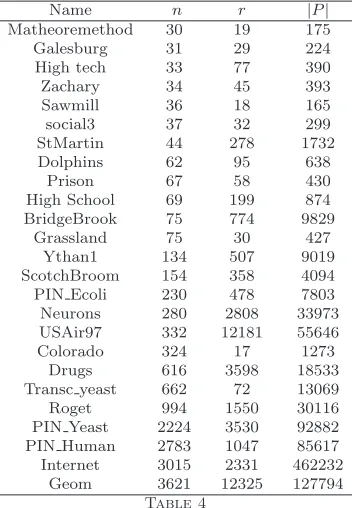
[image:17.612.212.388.96.350.2]Table 4
Dataset: nnumber of nodes in the network,rnumber of existing triangles, and|P|number of
open triads.
• PIN Human: protein-protein interaction network in human [50];
• PIN Yeast: protein-protein interaction network inS. cerevisiae(yeast) [7, 38].
Social and economic networks
• Colorado: the risk network of persons with HIV infection during its early epidemic phase in Colorado Spring, USA, using analysis of community wide HIV/AIDS contact tracing records (sexual and injecting drugs partners) from 1985-1999 [48];
• Dolphins: social network of frequent association between 62 bottlenose dol-phins living in the waters off New Zealand [33];
• Drugs: social network of injecting drug users (IDUs) that have shared a needle in the last six months [43].
• Galesburg: friendship ties among 31 physicians [10, 28, 46];
• Geom: collaboration network of scientists in the field of Computational Ge-ometry [3];
• High School: network of relations in a high school. The students choose the three members they wanted to have in a committee [56];
• High tech: friendship ties among the employees in a small high-tech computer firm which sells, installs, and maintain computer systems [29, 46];
• Matheoremethod: this network concerns the diffusion of a new mathematics method in the 1950s. It traces the diffusion of the modern mathematical method among school systems that combine elementary and secondary pro-grams in Allegheny County (Pennsylvania, U.S.) [9, 46];
• Sawmill: social communication network within a sawmill, where employees were asked to indicate the frequency with which they discussed work matters with each of their colleagues [39, 46];
• social3: social network among college students in a course about leadership. The students choose which three members they wanted to have in a committee [56];
• Zachary: social network of friendship among the members of a karate club [55].
Technological networks
• Internet: the Internet at the Autonomous System (AS) level as of September 1997 and of April 1998 [20];
• USAir97: airport transportation network between airports in US in 1997 [3].
Transcription networks
• Transc yeast: direct transcriptional regulation between genes inSaccaromyces cerevisiae [41, 42].
REFERENCES
[1] M. Benzi and G. H. Golub,Bounds for the entries of matrix functions with application to
preconditioning, BIT 39 (1999), pp. 417–438.
[2] M. Benzi and P. Boito,Quadrature rule-based bounds for functions of adjacency matrices, Linear Algebra Appl. 433 (2010), pp. 637–652.
[3] V. Batagelj and A. Mrvar,Pajek datasets, http://vlado.fmf.uni-lj.si/pub/networks/data/. [4] F. Battiston, V. Nicosia, and V. Latora, Biased random walks on multiplex networks,
arXiv:1505.01378 (2015).
[5] G. Bianconi, R. K. Darst, J. Iacovacci and S. Fortunato, Triadic closure as a basic
generating mechanism of communities in complex networks, Phys. Rev. E, 90 (4) (2014),
042806.
[6] S. Boccaletti, G. Bianconi, R. Criado, C. I. Del Genio, J. G´omez-Gardenes, M. Ro-mance, I. Sendina–Nadal, Z. Wang, and M. Zanin, The structure and dynamics of
multilayer networks, Phys. Rep. 544 (2014): pp. 1–122.
[7] D. Bu, Y. Zhao, L. Cai, H. Xue, X. Zhu, H. Lu, J. Zhang, S. Sun, L. Ling, N. Zhang, G. Li, and R. Chen,Topological structure analysis of the protein-protein interaction network in
budding yeast, Nucleic Acids Res. 31 (2003), pp. 2443–2450.
[8] G. Butland, J. M. Peregr´ın–Alvarez, J. Li, W. Yang, X. Yang, V. Canadien, A. Staros-tine, D. Richards, B. Beattie, N. Krogan, M. Davey, J. Parkinson, J. Greenblatt, and A. Emili,Interaction network containing conserved and essential protein complexes
in Escherichia coli, Nature 433.7025 (2005), pp. 531–537.
[9] R. O. Carlson,Adoption of Educational Innovations, Eugene: University of Oregon, Center for the Advanced Study of Educational Administration (1965), p. 19).
[10] J. S. Coleman, E. Katx, H. Menzel,Medical Innovation. A Diffusion Study, Indianapolis: Bobbs–Merrill Company, 1966.
[11] E. Cozzo, M. Kivel¨a, M. De Domenico, A. Sol´e, A. Arenas, S. G´omez, M. A. Porter, and Y. Moreno,Structure of Triadic Relations in Multiplex Networks, arXiv:1307.6780. [12] L. F. Costa, O. N. Oliveira Jr, G. Travieso, F. A. Rodrigues,P. R. Villas Boas, L.
An-tiqueira, M. P. Viana, and L. E. C. Rocha,Analyzing and modeling real-world
phenom-ena with complex networks: a survey of applications, Advances in Physics 60 (3) (2011),
pp. 329–412.
[13] E. Estrada and J. G´omez-Gardenes,Communicability reveals a transition to coordinated
behavior in multiplex networks, Phys. Rev. E 89(4) (2014): 042819.
[14] E. Estrada and N. Hatano,Communicability in Complex Networks, Phys. Rev. E, 77 (2008), 036111.
[15] E. Estrada, D. J. Higham, Network properties revealed through matrix functions, SIAM Rev. 52 (2010), pp. 696–714.
[17] E. Estrada, N. Hatano, M. Benzi,The physics of communicability in complex networks, Phys. Rep. 514 (2012), pp. 89–119.
[18] E. Estrada, The communicability distance in graphs, Linear Algebra Appl. , 436 (2012), pp. 4317–4328.
[19] E. Estrada, Complex networks in the Euclidean space of communicability distances, Phys. Rev. E, 85 (2012), 066122.
[20] M. Faloutsos, P. Faloutsos, and C. Faloutsos,On power-law relationships of the internet
topology, Comp. Comm. Rev. 29 (1999), pp. 251–262.
[21] G. H. Golub and G. Meurant,Matrices, Moments and Quadrature with Applications, Prince-ton University Press, PrincePrince-ton, NJ 2010.
[22] N. J. Higham,Functions of Matrices: Theory and Computation, Society for Industrial and Applied Mathematics, Philadelphia, PA, 2008.
[23] R. A. Horn and C. R. Johnson, Matrix Analysis. Second Edition, Cambridge University Press, 2013.
[24] H. Huang, J. Tang, S. Wu, L. Liu, and X. Fu, Mining triadic closure patterns in social
networks, Proceedings of the companion publication of the 23rd international conference
on World wide web companion. International World Wide Web Conferences Steering Com-mittee, 2014.
[25] M. Huxman, S. Beany, and D. Raffaelli,Do parasites reduce the chances of triangulation
in a real food web?, Oikos 76 (1996), pp. 284–300.
[26] M. Kivel¨a, A. Arenas, M. Barthelemy, J. P. Gleeson, Y. Moreno, and M. A. Porter,
Multilayer networks, J. Complex Networks 2(3) (2014), pp. 203–271.
[27] P. Klimek and S. Thurner,Triadic closure dynamics drives scaling laws in social multiplex
networks, New Journal of Physics 15.6 (2013): 063008.
[28] D. Knoke and R. S. Burt,Prominence, Applied network analysis (1983): pp. 195–222. [29] D. Krackhardt, The ties that torture: Simmelian tie analysis in organizations, Res.
So-ciol. Org. 16 (1999), pp. 183–210.
[30] D. Krackhardt and M. Handcock, Heider vs. Simmel: Emergent features in dynamic
structure, Statistical Network Analysis: Models, Issues, and New Directions (2007), pp. 14–
27.
[31] J. Leskovec, L. Backstrom, R. Kumar, A. Tomkins,Microscopic evolution of social
net-works, Y. Li, B. Liu, S. Sarawagi (eds.) KDD, pp. 462–470, ACM (2008).
[32] T. Lou, J. Tiancheng, J. Hopcroft, Z. Fang, and X. Ding,Learning to predict reciprocity
and triadic closure in social networks, ACM Transactions on Knowledge Discovery from
Data (TKDD) 7.2 (2013).
[33] D. Lusseau, K. Schneider, O. J. Boisseau, P. Haase, E. Slooten, and S. M. Dawson,The bottlenose dolphin community in Doubtful Sound features a large proportion of long-lasting
associations, Behavioral Ecology and Sociobiology 54 (2003), pp. 396–405.
[34] D. MacRae,Direct factor analysis of sociometric data, Sociometry 23 (1960), pp. 360–371. [35] N. D. MartinezArtifacts or attributes? Effects of the resolution on the Little Rock lake food
web, Ecol. Monogr. 61 (1991), pp. 367–392.
[36] N. D. Martinez, B. A. Hawkins, H. A. Dawah, and B. P. Feifarek,Effects of sampling
efforts on characterization of food web structure, Ecology 80 (1999), pp. 1044–1055.
[37] J. Memmott, N. D. Martinez, and J. E. Cohen, Predators, parasitoids and pathogens:
species richness, trophic generality and body sizes in a natural food web, J. Anim. Ecol. 69. 1
(2000), pp. 1–15.
[38] C. von Mering, R. Krause, B. Snel, M. Cornell, S. G. Oliver, S. Fields, and P. Bork,
Comparative assessment of large-scale data sets of protein-protein interactions, Nature
417 (2002), pp. 399–403.
[39] J. H. Michael and J. G. Massey,Modeling the communication network in a sawmill, Forest Prod. J. 47 (1997), pp. 25–30.
[40] P. Van Mieghem,Graph Spectra for Complex Networks, Cambridge University Press, 2011. [41] R. Milo, S. Shen–Orr, S. Itzkovitz, N. Kashtan, D. Chklovskii, and U. AlonNetwork
motifs: simple building blocks of complex networks, Science, vol. 298 no. 5594 (2002),
pp. 824–827.
[42] R. Milo, S. Itzkovitz, N. Kashtan, R. Levitt, S. S. Shen–Orr, I. Ayzenshtat, M. Shef-fer, and U. Alon, Superfamilies of evolved and designed networks, Science 303.5663 (2004), pp. 1538–1542.
[43] Data for this project were provided, in part, by NIH grants DA12831 and HD41877, and copies can be obtained from James Moody ([email protected]).
[45] M. E. J. Newman,Networks. An Introduction, Oxford University Press, 2010.
[46] W. De Nooy, A. Mrvar, and V. Batagelj,Exploratory Social Network Analysis with Pajek, Cambridge University Press, 2005.
[47] G. A. Polis and R. S. Donald, Food web complexity and community dynamics, Am. Nat. (1996): pp. 813-846.
[48] J. J. Potterat, L. Philips–Plummer, S. Q. Muth, R. B. Rothenberg, D. E. Woodhouse, T. S. Maldonado–Long, H. P. Zimmermann, J. B. Muth,Risk network structure in the
early epidemic phase of HIV transmission in Colorado Springs, Sex. Transm. Infect. 78
(2002), pp. i159–i163.
[49] Roget’s thesaurus of english words and phrases, Project Gutenberg (2002),
http://www.gutenberg.org/etxt/22.
[50] J. F. Rual, K. Venkatesan, T. Hao, T. Hirozante–Kishikawa, A. Dricot, L. Ning, G. F. Berriz, F. D. Gibbons, M. Dreze, N. Ayivi–Guedehoussou, N. Klitgord, C. Si-mon, M. Boxem, S. Milstein, J. Rosenberg, D. S. Goldberg, L. V. Zhang, S. L. Wong, G. Franklin, S. Li, J. S. Albala, J. Lim, C. Fraughton, E. Llamosas, S. Cevik, P. Lamesch, R. S. sikoroski, J. Andenhaute, H. Y. Zoghbi, A. Smolyar, S. Bosak, R. Sequerra, L. Doucette–Stamm, M. E. Cusick, D. E. Hill, F. P. Roth, and M.
Vi-dal,Towards a proteome-scale map of the human protein-protein interaction networks,
Nature 437 (2005), pp. 1059–1069.
[51] P. Sen and B. K. Chakrabarti,Sociophysics. An Introduction., Oxford University Press, Oxford, (2014).
[52] G. Simmel,Conflict and The Web of Group Affiliations, Free Press, New York (1922). [53] D. J. Watts and S. H. Strogatz,Collective dynamics of small-world networks, Nature 393
(1998), pp. 440–442.
[54] J. G. White, E. Southgate, J. N. Thomson, and S. BrennerThe structure of the nervous
system of the nematode Caenorhabditis elegans, Philos. T. Roy. Soc. B, 314.1165 (1986),
pp. 1-340.
[55] W. W. Zachary,An information flow model for conflict and fission in small groups, J. An-thropol. Res., 33 (1977), pp. 452–473.
[56] L. D. Zeleny,Adaptation of research findings in social leadership to college classroom