City, University of London Institutional Repository
Citation
:
Balasubramanian, V., de Boer, J., Feng, B., He, Y., Huang, M., Jejjala, V. and Naqvi, A. (2003). Multitrace superpotentials vs. matrix models. Communications inMathematical Physics, 242, pp. 361-392. doi: 10.1007/s00220-003-0947-9
This is the unspecified version of the paper.
This version of the publication may differ from the final published
version.
Permanent repository link: http://openaccess.city.ac.uk/841/
Link to published version
:
http://dx.doi.org/10.1007/s00220-003-0947-9Copyright and reuse:
City Research Online aims to make research
outputs of City, University of London available to a wider audience.
Copyright and Moral Rights remain with the author(s) and/or copyright
holders. URLs from City Research Online may be freely distributed and
linked to.
arXiv:hep-th/0212082v3 13 Dec 2002
Preprint typeset in JHEP style - HYPER VERSION UPR-1025-T, ITFA-2002-57
VPI-IPPAP-02-17, hep-th/0212082
Multi-Trace Superpotentials vs. Matrix Models
Vijay Balasubramanian1, Jan de Boer2, Bo Feng3, Yang-Hui He1, Min-xin Huang1, Vishnu
Jejjala4, and Asad Naqvi1
1. David Rittenhouse Laboratories, The University of Pennsylvania,
209 S. 33rd St., Philadelphia, PA 19104-6396
2. Institute of Theoretical Physics, University of Amsterdam,
Valckenierstraat 65, 1018 XE, Amsterdam, The Netherlands
3. Institute for Advanced Study, Olden Lane, Princeton, NJ 08540
4. Institute for Particle Physics and Astrophysics Department of Physics, Virginia Tech
Blacksburg, VA 24061
[email protected],[email protected],[email protected],[email protected], [email protected],[email protected],[email protected]
Abstract:We considerN = 1 supersymmetricU(N) field theories in four dimensions with adjoint
chiral matter and a multi-trace tree-level superpotential. We show that the computation of the effective action as a function of the glueball superfield localizes to computing matrix integrals. Unlike the single-trace case, holomorphy and symmetries do not forbid non-planar contributions. Nevertheless, only a special subset of the planar diagrams contributes to the exact result. Some of the data of this subset can be computed from the large-N limit of an associated multi-trace Matrix model. However, the prescription differs in important respects from that of Dijkgraaf and Vafa for single-trace superpotentials in that the field theory effective action is not the derivative of a multi-trace matrix model free energy. The basic subtlety involves the correct identification of the field theory glueball as a variable in the Matrix model, as we show via an auxiliary construction involving a single-trace matrix model with additional singlet fields which are integrated out to compute the multi-trace results. Along the way we also describe a general technique for computing the large-N limits of multi-trace Matrix models and raise the challenge of finding the field theories whose effective actions they may compute. Since our models can be treated asN = 1 deformations of pureN = 2 gauge theory, we show that the effective superpotential that we compute also follows from the N = 2 Seiberg-Witten solution. Finally, we observe an interesting connection between multi-trace local theories and non-local field theory.
Contents
1. Introduction 1
2. Multi-Trace Superpotentials from Perturbation Theory 4
2.1 A Schematic Review of the Field Theory Superpotential Computation 4 2.2 Computation of a Multi-Trace Superpotential 8 2.3 Which Diagrams Contribute: Selection Rules 11
2.4 Summing Pasted Diagrams 13
2.5 Perturbative Calculation 15
2.5.1 First Order 15
2.5.2 Second Order 15
2.5.3 Third Order 16
2.5.4 Obtaining the Effective Action 16
2.6 Multiple Traces, Pasted Diagrams and Nonlocality 18
3. The Field Theory Analysis 18
3.1 The Classical Vacua 19
3.2 The Exact Superpotential in the Confining Vacuum 20
3.3 An Explicit Example 22
4. The Matrix Model 23
4.1 The Mean-Field Method 23
4.2 Generalized Multi-Trace Deformations 25
5. Linearizing Traces: How To Identify the Glueball? 27
5.1 Field Theory Computation ofWsingle(A,S) and Pasted Matrix Diagrams 27
5.2 Matrix model perspective 29
5.3 General Multi-trace Operators 30
6. Conclusion 31
1. Introduction
of stringy dualities arising in context of geometrically engineered field theories, two recent papers have suggested direct field theory proofs of the proposal [4, 5]. These works considered U(N) gauge theories with an adjoint chiral matter multiplet Φ and a tree-level superpotential W(Φ) =
P
kgkTr(Φk). Using somewhat different techniques ([4] uses properties of superspace perturbation
theory while [5] relies on factorization of chiral correlation functions, symmetries, and the Konishi anomaly) these papers conclude that:
1. The computation of the effective superpotential as a function of the glueball superfield reduces to computing matrix integrals.
2. Because of holomorphy and symmetries (or properties of superspace perturbation theory), only planar Feynman diagrams contribute.
3. These diagrams can be summed up by the large-N limit of an auxiliary Matrix model. The field theory effective action is obtained as a derivative of the Matrix model free energy. Various generalizations and extensions of these ideas (e.g., N = 1∗ theories [6, 7], fundamental matter [8, 9], quantum moduli spaces [10], non-supersymmetric cases [11], other gauge groups [12, 13, 14, 15], baryonic matter [16, 17], gravitational corrections [18, 19], and Seiberg Duality [20, 21]) have been considered in the recent literature.
A stringent and simple test of the Dijkgraaf-Vafa proposal and of the proofs presented in [4, 5] is to consider superpotentials containing multi-trace terms such as
W(Φ) =g2Tr(Φ2) +g4Tr(Φ4) +eg2(Tr(Φ2))2. (1.1)
We will show that for such multi-trace theories:
1. The computation of the effective superpotential as a function of the glueball superfield still reduces to computing matrix integrals.
2. Holomorphy and symmetries do not forbid non-planar contributions; nevertheless only a certain subset of the planar diagrams contributes to the effective superpotential.
3. This subclass of planar graphs also contributes to the large-N limit of an associated multi-trace Matrix model. However, because of differences in combinatorial factors, the field theory effective superpotential cannot be obtained simply as a derivative of the multi-trace Matrix model free energy as in [3].
4. Multi-trace theories can be linearized in traces by the addition of auxiliary singlet fieldsAi.
The superpotentials for these theories as a function of both the Ai and the glueball can be
our understanding of the selection rules determining which perturbative field theory diagrams contribute to the effective superpotential of an N = 1 field theory. Using this understanding we demonstrate how the conclusions (1) and (2) above arise and show that contributing diagrams are tree-like graphs in which single-trace diagrams are pasted together by double-trace vertices through which no momentum flows. We illustrate our results by explicitly computing the superpotential to the first few orders in perturbation theory. Finally, we observe an intriguing connection between multi-trace local theories and non-local field theory.
Since the field content of pure N = 2 supersymmetric U(N) gauge theory in four dimensions consists in N = 1 language of a vector multiplet Wα and an adjoint chiral multiplet Φ, the
superpotential (1.1) can be treated as a deformation of an N = 2 theory to an N = 1 theory. Hence, we can use global symmetries, holomorphy, regularity conditions, and the Seiberg-Witten solution ofN = 2 gauge theory to compute the exact superpotential. We carry out this procedure in Sec. 3, using the fact that the vacuum expectation value of the product of chiral operatorshTr(Φ2)2i factorizes ashTr(Φ2)i2. We show that the result exactly captures the subset of the planar diagrams
that contribute to the exact field theory superpotential. The assumption of factorization in the Seiberg-Witten analysis is equivalent to the vanishing of a certain subset of planar diagrams in our perturbative computations.
In Sec. 4 we demonstrate a general technique for solving U(M) matrix models (or general complex matrix models) with multi-trace potentials. The essential observation, following Das, Dhar, Sengupta, and Wadia [22], is that in the large-M limit, mean field methods can be used to solve for the effect on a single matrix eigenvalue of the rest of the matrix. We explain the general method and solve two examples in detail. The first example has a potential V(Φ) = M(g2Tr(Φ2) +g4Tr(Φ4) +Meg2Tr(Φ2)2) for φ ∈ U(M). By expanding the exact large-M result in
powers of the couplings we demonstrate how this limit computes the data relevant for a certain subset of the planar contributions to the effective action of the field theory with the tree-level superpotential in (1.1). In the proposal of Dijkgraaf and Vafa [3] and the subsequent generalizations (e.g., [6] to [21]), the field theory effective action was related simply to the free energies of auxiliary matrix models and their derivatives. We demonstrate the absence of such a relation between multi-trace field theories and multi-multi-trace Matrix models. As a further illustration of the mean field technique for computing large-M limits, we study a matrix model with a general quartic potential. Multi-trace field theories can be linearized in traces by the introduction of new singlet fields which can be integrated out to produce the multi-trace theory. In Sec. 5 we show how this procedure is carried out and relate the resulting linearized superpotential to a Matrix model following the techniques of [4]. In the Matrix model integrating out the singlets at the level of the free energy reproduces the multi-trace results that do not agree with the field theory. However, integrating out after computing the linearized field theory superpotential leads to agreement. This shows that the basic subtlety here involves the correct identification of the field theory glueball as a variable in an associated Matrix moedl.
ad-joint matter involves multi-trace superpotentials, and therefore these deformations are important to understand. What is more, multi-trace superpotentials cannot be geometrically engineered [23] in the usual manner for a simple reason: in geometric engineering of gauge theories the tree-level superpotential arises from a disc diagram for open strings on a D-brane and these, having only one boundary, produce single-trace terms. In this context, even if multi-trace terms could be produced by quantum corrections, their coefficients would be determined by the tree-level couplings and would not be freely tunable. Hence comparison of the low-energy physics arising from multi-trace superpotentials with the corresponding Matrix model calculations is a useful probe of the extent to which the Dijkgraaf-Vafa proposal is tied to its geometric and D-brane origins. In addition to these motivations, it is worth recalling that the double scaling limit of the U(N) matrix model with a double-trace potential is related to a theory of two-dimensional gravity with a cosmological constant. This matrix model also displays phase transitions between smooth, branched polymer and intermediate phases [22]. It would be interesting to understand whether and how these phe-nomena manifest themselves as effects in a four dimensional field theory. The results of our paper suggest that these phase transitions and the physics of two-dimensional cosmological constants are embedded within four-dimensional field theory. It would be interesting to explore this. Finally, multi-trace deformations of field theories have recently made an appearance in the contexts of the AdS/CFT correspondence and a proposed definition of string theories with a nonlocal worldsheet theory [24].
2. Multi-Trace Superpotentials from Perturbation Theory
In this section we begin by reviewing the field theoretic proof that when treated as a function of the glueball superfield, the effective superpotential of an N = 1 supersymmetric gauge theory with single-trace tree-level interactions is computed by planar matrix diagrams [4, 5]. We will then describe how these arguments are modified by the presence of multi-trace terms in the tree-level action. Finally, we will explicitly illustrate our reasoning by perturbatively computing the diagrams that contribute to the effective superpotential of a multi-trace theory up to third order in the couplings. We will always work around a vacuum with unbrokenU(N) symmetry.
2.1 A Schematic Review of the Field Theory Superpotential Computation
Below we give a schematic description of the methods of [4] for the computation of the effective superpotential of anN = 1 field theory. While [4] discussed theories with single-trace Lagrangians, we will find that most of their arguments will generalize easily to multi-trace theories.
1. The Action: The matter action for an N = 1 U(N) gauge theory with a vector multipletV, a massive chiral superfield Φ, and superpotentialW(Φ), is given in superspace by
S(Φ,Φ) =¯
Z
d4x d4θΦe¯ VΦ +
Z
2. The Goal: We seek to compute the effective superpotential as a function of the glueball superfield
S= 1
32π2Tr(W
αW
α), (2.2)
where
Wα =iD
2
e−VDαeV (2.3)
is the gauge field strength ofV, withDα=∂/∂θα and Dα˙ =∂/∂θ¯α˙+iθα∂αα˙ the superspace
covariant derivatives, and D2 = 12DαDα and D2 = 12Dα˙Dα˙. The gluino condensate S is a
commuting field constructed out of a pair of fermionic operatorsWα.
3. The Power of Holomorphy: We are interested in expressing the effective superpotential in terms of the chiral glueball superfield S. Holomorphy tells us that it will be independent of the parameters of the anti-holomorphic part of the tree-level superpotential. Therefore, without loss of generality, we can choose a particularly simple form forW( ¯Φ):
W( ¯Φ) = 1 2mΦ¯
2. (2.4)
Integrating out the anti-holomorphic fields and performing standard superspace manipula-tions as discussed in Sec. 2 of [4], gives
S =
Z
d4xd2θ
−2m1 Φ (−iWαDα) Φ +Wtree(Φ)
(2.5) as the part of the action that is relevant for computing the effective potential as a function of S. Here, = 12∂αα˙∂αα˙ is the d’Alembertian, and Wtree is the tree-level superpotential,
expanded as 12mΦ2+ interactions. (The reader may consult Sec. 2 of [4] for a discussion of various subtleties such as why thecan be taken as the ordinary d’Alembertian as opposed to a gauge covariantized cov).
4. The Propagator: After reduction into the form (2.5), the quadratic part gives the propaga-tor. We write the covariant derivative in terms of Grassmann momentum variables
Dα=∂/∂θα :=−iπα, (2.6)
and it has been shown in [4] that by rescaling the momenta we can put m = 1 since all m dependence cancels out. Then the momentum space representation of the propagator is simply
Z ∞
0
dsi exp −si(p2i +Wαπiα+m)
, (2.7)
wheresi is the Schwinger time parameter ofi-th Feynman propagator. Here the precise form
of the Wαπ
α depends on the representation of the gauge group that is carried by the field
5. Calculation of Feynman Diagrams: The effective superpotential as a function of the glue-ballSis a sum of vacuum Feynman diagrams computed in the background of a fixed constant
Wα leading to insertions of this field along propagators. In general there will beℓmomentum
loops, and the corresponding momenta must be integrated over yielding the contribution I =
Z Y
a,i
d4padsie−sip
2
i ·
Z Y
a,i
d2πadsie−siW
α
πiα
· Z Y i
dsie−sim !
=Iboson·If ermion·
1
mP (2.8)
to the overall amplitude. Herea labels momentum loops, whilei= 1, . . . , P labels propaga-tors. The momenta in the propagators are linear combinations of the loop momenta because of momentum conservation.
6. Bosonic Momentum Integrations: The bosonic contribution can be expressed as
Iboson =
Z Yℓ
a=1
d4pa
(2π)4 exp
−X a,b
paMab(s)pb
= 1 (4π)2ℓ
1
(detM(s))2, (2.9)
where we have defined the momentum of the i-th propagator in terms of the independent loop momentapa
pi= X
a
Liapa (2.10)
via the matrix elementsLia ∈ {0,±1} and
Mab(s) = X
i
siLiaLib. (2.11)
7. Which Diagrams Contribute: Since each momentum loop comes with two fermionic πα
integrations (2.8) a non-zero amplitude will require the insertion of 2ℓ παs. From (2.7) we
see that thatπα insertions arise from the power series expansion of the fermionic part of the
propagator and that each πα is accompanied by a Wα. So in total we expect an amplitude
containing 2ℓfactors ofWα. Furthermore, since we wish to compute the superpotential as a
function of S∼Tr(WαWα) each index loop can only have zero or two Wα insertions. These
considerations together imply that if a diagram contributes to the effective superpotential as function of theS, then number of index loopshmust be greater than or equal to the number of momentum loops ℓ,i.e.,
h≥ℓ. (2.12)
8. Planarity: The above considerations are completely general. Now let us specialize to U(N) theories with single-trace operators. A diagram withℓmomentum loops has
h=ℓ+ 1−2g (2.13)
9. Doing The Fermionic Integrations: First let us discuss the combinatorial factors that arise from the fermionic integrations. Since the number of momentum loops is one less than the number of index loops, we must choose which of the latter to leave free ofWα insertions.
This gives a combinatorial factor ofh, and the empty index loop gives a factor ofN from the sum over color. For each loop with two Wα insertions we get a factor of 12WαWα = 16π2S.
Since we are dealing with adjoint matter, the action ofWα is through a commutator
exp (−si[Wiα,−]πiα) (2.14)
in the Schwinger term. (See the appendix of [12] for a nice explanation of this notation as it appears in [4]. In Sec. 2.2 we will give an alternative discussion of the fermionic integrations that clarifies various points.) As in the bosonic integrals above, it is convenient to express the fermionic propagator momenta as sums of the independent loop momenta:
πiα = X
a
Liaπaα, (2.15)
where theLiaare the same matrix elements as introduced above. The authors of [4] also find
it convenient to introduce auxiliary fermionic variables via the equation
Wα
i =
X
a
LiaWaα. (2.16)
Here, theLia =±1 denotes the left- or right-action of the commutator. In terms of theWaα,
the fermionic contribution to the amplitude can be written as
If ermion = N h(16π2S)ℓ
Z Y
a
d2πad2Wa exp
−X a,b
WaαMab(s)πbα
= (4π)2ℓN hSℓ(detM(s))2. (2.17)
10. Localization: The Schwinger parameter dependence in the bosonic and fermionic momen-tum integrations cancel exactly
Iboson·If ermion=N hSℓ, (2.18)
implying that the computation of the effective superpotential as a function of theS localizes to summing matrix integrals. All the four-dimensional spacetime dependence has washed out. The full effective superpotentialWef f(S) is thus a sum over planar matrix graphs with
the addition of the Veneziano-Yankielowicz term for the pure Yang-Mills theory [25]. The terms in the effective action proportional to Sℓ arise exclusively from planar graphs with ℓ momentum loops giving a perturbative computation of theexact superpotential.
limit of a bosonic Matrix model. (We distinguish betweenM, the rank of the matrices in the Matrix model and N, the rank of the gauge group.) The prescription of Dijkgraaf and Vafa does exactly this for single-trace superpotentials. Since the number of momentum loops is one less than the number of index loops in a planar diagram, the net result of the bosonic and fermionic integrations in (2.18) can be written as
Iboson·If ermion=N
∂Sh
∂S . (2.19)
Because of this, the perturbative part of the effective superpotential, namely the sum over planar diagrams in the field theory, can be written in terms of the genus zero free energy
F0(S) of the corresponding matrix model:
Wpert(S) = N
∂
∂SF0(S), (2.20)
F0(S) =
X
h
F0,hSh. (2.21)
This free energy is conveniently isolated by taking the large-M limit of the zero-dimensional one-matrix model withM ×M matrices1 Φ and potentialW(Φ) whose partition function is given by
Z = exp(M2F0) =
1 Vol(U(M))
Z
[DΦ] exp
−1
gs
TrW(Φ)
. (2.22)
In this matrix model every index loop gives a power ofM just as in the field theory compu-tation, and all but one index loop gives a power ofS. Because of this simple fact the powers of the gluino condensate in the field theory superpotential can be conveniently counted by identifying it with the ’t Hooft couplingS≡M gs, and then differentiating the matrix model
free energy as in (2.20). Rather surprisingly the Veneziano-Yankielowicz term in Wef f(S)
arises from the volume factor in the integration over matrices in (2.22).
One important unanswered question is why the low-energy dynamics simplifies so much when written in terms of the gluino condensates.
2.2 Computation of a Multi-Trace Superpotential
We have reviewed above how the field theory calculation of the effective superpotential for a single-trace theory localizes to a matrix model computation. In this subsection we show how the argument is modified when the tree-level superpotential includes multi-trace terms. We consider an N = 1 theory with the tree-level superpotential
Wtree=
1 2Tr(Φ
2) +g
4Tr(Φ4) +eg2(Tr(Φ2))2 . (2.23) 1The original papers of Dijkgraaf and Vafa [1, 2] consider
M ×M Hermitian matrices (i.e. matrices with real eigenvalues λi). In fact, we should think of the matrices as belonging to GL(M,C) with eigenvalues distributed
To set the stage for our perturbative computation of the effective superpotential we begin by analyzing the structure of the new diagrams introduced by the double-trace term. If eg2 = 0, the
connected diagrams we get are the familiar single-trace ones; we will call theseprimitive diagrams. When eg2 6= 0 propagators in primitive diagrams can be spliced together by new double-trace
vertices. It is useful to do an explicit example to see how this splicing occurs. As an example, let
x
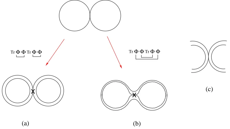
x
TrΦ ΦTrΦ Φ TrΦ ΦTrΦ Φ
(a) (b)
[image:11.612.119.495.169.380.2](c)
Figure 1: Two ways in which the double-trace operator: Tr(Φ2)Tr(Φ2) can be contracted using the vertex
shown in (c).
us study the expectation value of the double-trace operator: hTr(Φ2)Tr(Φ2)i. To lowest order in couplings, the two ways to contract Φs give rise to the two diagrams in Figure 1. When we draw these diagrams in double line notation, we find that Figure 1a corresponding to Tr(ΦΦ)Tr(ΦΦ) has four index loops, while Figure 1b corresponding to Tr(Φ Φ)Tr(Φ Φ) has only two index loops. Both these graphs have two momentum loops. For our purposes both of these Feynman diagrams can also be generated by a simple pictorial algorithm: we splice together propagators of primitive diagrams using the vertex in Figure 1c, as displayed in Figure 2a and b. All graphs of the double-trace theory can be generated from primitive diagrams by this simple algorithm. Note that the number of index loops never changes when primitive diagrams are spliced by this pictorial algorithm.
(a) Paste (b) Pinch
[image:12.612.159.456.73.303.2]x
x
Figure 2: With the inclusion of the double-trace term we need new types of vertices. These can be obtained from the “primitive” diagrams associated with the pure single-trace superpotential by (a) pasting or (b) pinching. The vertices have been marked with a cross.
x
x
x
x
x
x
Figure 3: More examples of “pinched” diagrams.
To make the above statement more clear, let us provide some calculations. First, according to our operation, the number of double index loops never increases whether under pasting or pinching. Second, we can calculate the total number of independent momentum loops ℓ by ℓ = P −V + 1 where P is the number of propagators and V, the number of vertices. If we connect two separate diagrams by pasting, we will have Ptot= (P1−1) + (P2−1) + 4, Vtot =V1+V2+ 1 and
ℓtot =Ptot−Vtot+ 1 =ℓ1+ℓ2, (2.24)
which means that the total number of momentum loops is just the sum of the individual ones. If we insert the double-trace vertex in a single connected diagram by pinching, we will have Ptot =
P−2 + 4,Vtot=V + 1, and
ℓtot=Ptot−Vtot+ 1 =ℓ+ 1, (2.25)
[image:12.612.169.448.369.483.2]Having understood the structure of double-trace diagrams in this way, we can adapt the tech-niques of [4] to our case. The steps 1-6 as described in Sec. 2.1 go through without modification since they are independent of the details of the tree-level superpotential. However the steps 7-11 are modified in various ways. First of all naive counting of powers of fermionic momenta as in step 7 leads to the selection rule
h≥ℓ, (2.26)
where h is the total number of index loops and ℓ is the total number of momentum loops. (The holomorphy and symmetry based arguments of [5] would lead to the same conclusion.) Since no momentum flows between pasted primitive diagrams it is clear that this selection rule would permit some of the primitive components to be non-planar. Likewise, both planar and some non-planar pinching diagrams are admitted. An example of a planar pinching diagram that can contribute according to this rule is Figure 2b. However, we will show in the next subsection that more careful consideration of the structure of perturbative diagrams shows that only diagrams built by pasting planar primitive graphs give non-zero contributions to the effective superpotential.
2.3 Which Diagrams Contribute: Selection Rules
In order to explain which diagrams give non-zero contributions to the multi-trace superpotential it is useful to first give another perspective on the fermionic momentum integrations described in steps 7–9 above. A key step in the argument of [4] was to split the glueball insertions up in terms of auxiliary fermionic variables associated with each of the momentum loops as in (2.16). We will take a somewhat different approach. In the end we want to attach zero or two fields Wα
(p) to eachindex
loop, where p labels the index loop, and the total number of such fields must bring down enough fermionic momenta to soak up the corresponding integrations. On each oriented propagator, with momentum πiα, we have a left index line which we labelpL and a right index line which we label
pR. Because of the commutator in (2.14), the contribution of this propagator will be
exp(−si(πiα(W(αpL)− W
α
(pR))). (2.27)
Notice that we are omitting U(N) indices, which are simply replaced by the different index loop labels. In a standard planar diagram for a single-trace theory, we have one more index loop than momentum loop. So even in this case the choice of auxiliary variables in (2.27) is not quite the same as in (2.16), since the number of Wαs is twice the number of index loops in (2.27) while the
number of auxiliary variables is twice the number of momentum loops in (2.16).
Now in order to soak up the fermionicπ integrations in (2.8), we must expand (2.27) in powers and extract terms of the form
W(2p1)W(2p2). . .W(2pl), (2.28)
whereℓis the number of momentum loops and all thepi are distinct. The range ofpis over 1, . . . , h,
withh the number of index loops. In the integral over the anticommuting momenta, we have allh
W(p) appearing. However, one linear combination, which is the ‘center of mass’ of the W(p), does
propagators do not change. Thus, without loss of generality, one can set the W(p) corresponding to the outer loop in a planar diagram equal to zero. Let us assume this variable is W(h) and later
reinstate it. AllW(p) corresponding to inner index loops remain, leaving as many of these as there are momentum loops in a planar diagram. It is then straightforward to demonstrate that the W
appearing in (2.16) in linear combinations reproduce the relations between propagator momenta and loop momenta. In other words, in this “gauge” where theW corresponding to the outer loop is zero, we recover the decomposition of Wα in terms of auxiliary fermions associated to momentum
loops that was used in [4] and reviewed in (2.16) above.
We can now reproduce the overall factors arising from the fermionic integrations in the planar diagrams contributing to (2.17). The result from theπ integrations is some constant times
ℓ Y
p=1
W(2p). (2.29)
Reinstating W(h) by undoing the gauge choice, namely by shifting
W(p)→ W(p)+W(h) (2.30)
forp= 1, . . . , h−1, (2.29) becomes
ℓ Y
p=1
(W(p)+W(h))2. (2.31) The terms on which each index loop there has either zero or twoW insertions are easily extracted:
h X
k=1
Y p6=k
W(2p)
. (2.32)
In this final result we should replace each of theW2
(p) by S, and therefore the final result is of the
form
hSh−1, (2.33)
as derived in [4] and reproduced in (2.17).
Having reproduced the result for single-trace theories we can easily show that all non-planar and pinched contributions to the multi-trace effective superpotential vanish. Consider any diagram withℓmomentum loops and hindex loops. By the same arguments as above, we attach someW(p)
to each index loop as in (2.27), and again, the ‘center of mass’ decouples due to the commutator nature of the propagator. Therefore, in the momentum integrals, only h−1 inequivalent W(p)
appear. By doing ℓ momentum integrals, we generate a polynomial of order 2ℓ in the h −1 inequivalent Wα
(p). This polynomial can by Fermi statistics only be non-zero if ℓ≤h−1: W(3p) is
zero for all p. Therefore, we reach the important conclusion that the total number of index loops must be larger than the number of momentum loops
while the naive selection rule (2.26) says that it could be larger or equal.
Consider pasting and pinching kprimitive diagrams together, each with hi index loops andℓi
momentum loops. According to the rules set out in the previous subsection, the total number of index loops and the total number of momentum loops are given by:
h=X
i
hi ; ℓ≥ X
i
ℓi (2.35)
with equality only when all the primitive diagrams are pasted together without additional momen-tum loops. Now the total number of independent Ws that appear in full diagram is Pi(hi−1)
since in each primitive diagram the “center of mass” W will not appear. So the full diagram is non-vanishing only when
ℓ≤X
i
(hi−1). (2.36)
This inequality is already saturated by the momenta appearing in the primitive diagrams if they are planar. So we can conclude two things. First, only planar primitive diagrams appear in the full diagram. Second, only pasted diagrams are non-vanishing, since pinching introduces additional momentum loops which would violate this inequality.
Summary: The only diagrams that contribute to the effective multi-trace superpotential are pastings of planar primitive diagrams. These are tree-like diagrams which string together double-trace vertices with “propagators” and “external legs” which are themselves primitive diagrams of the single-trace theory. Below we will explicitly evaluate such diagrams and raise the question of whether there is a generating functional for them.
2.4 Summing Pasted Diagrams
In the previous section we generalized steps 7 and 8 of the the single trace case in Sec. 2.1 to the double-trace theory, and found that the surviving diagrams consist of planar connected primitive vacuum graphs pasted together with double-trace vertices. Because of momentum conservation, no momentum can flow through the double-trace vertices in such graphs. Consequently the fermionic integrations and the proof of localization can be carried out separately for each primitive grapg, and the entire diagram evaluates to a product of the the primitive components times a suitable power ofge2, the double-trace coupling.
Let Gi,i= 1, . . . , k be the planar primitive graphs that have been pasted together, each with
hi index loops andℓi = hi−1 momentum loops to make a double-trace diagram G. Then, using
the result (2.18) for the single-trace case, the Schwinger parameters in the bosonic and fermionic momentum integrations cancel giving a factor
Iboson·If ermion=
Y
i
(N hiSℓi) =NkS
P
i(hi−1)Y
i
hi, (2.37)
k(G) as the number of primitive components,h(G) =Pihi as the total number of index loops and
ℓ(G) =Piℓi =h(G)−k(G) as the total number of momentum loops, we get
Iboson·If ermion =
Y
i
(N hiSiℓ) =Nh(G)−ℓ(G)Sl(G)C(G). (2.38)
We can assemble this with the Veneziano-Yankielowicz contribution contribution for pure gauge theory [25] to write the complete glueball effective action as
Wef f =−N S(log(S/Λ2)−1) + X
G
C(G)F(G)Nh(G)−ℓ(G)Sℓ(G), (2.39)
where F(G) is the combinatorial factor for generating the graph G from the Feynman diagrams of the double-trace theory. Notice that in our discussion, we have set g2 = m = 1, so Λ2 in this
equation is in fact mΛ2 which matches the dimension ofS. We can define a free energy related to
above diagrams as
F0 =
X
G
F(G)Sh(G). (2.40)
F0 is a generating function for the diagrams that contribute to the effective superpotential, but
does not include the combinatorial factors arising from the glueball insertions. In the single-trace case that combinatorial factor was simplyN h(G) and so we could writeWef f =N(∂F0/∂S). Here
C(G) = Qhi is a product rather than a sum h(G) = Phi, and so the effective superpotential
cannot be written as a derivative of the free energy.
Notice that if we rescale eg2 toeg2/N, there will be aN−(k(G)−1) factor fromk(G)−1 insertions
of the double-trace vertex. This factor will change the Nh(G)−l(G) dependence in (2.39) to just N for every diagram. This implies that the matrix diagrams contributing to the superpotential are exactly those that survive the large M limit of a bosonicU(M) Matrix model with a potential
V(Φ) =g2Tr(Φ2) +g4Tr(Φ4) + e
g2
MTr(Φ
2)Tr(Φ2). (2.41)
In Sec. 4 we will compute the largeM limit of a such a Matrix model and compute the free energy
F0 in this way.
2.5 Perturbative Calculation
Thus equipped, let us begin our explicit perturbation calculations. We shall tabulate all combi-natoric data of the pasting diagrams up to third order. Here C(G) =Qihi and F(G) is obtained
by counting the contractions of Φs. For pure single-trace diagrams the values of F(G) have been computed in Table 1 in [26], so we can utilize their results.
2.5.1 First Order
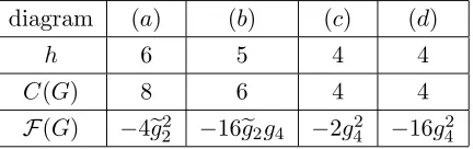
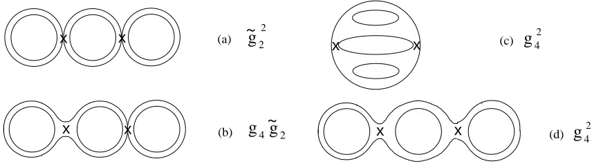
To first order in coupling constants, all primitive (diagram (b)) and pasting diagrams (diagram (a)) are presented in Figure 4. Let us illustrate by showing the computations for (a). There is a total of four index loops and henceh= 4 for this diagram. Moreover, since it is composed of the pasting of two primitive diagrams each of which has h= 2; thus, we have C(G) = 2×2 = 4. Finally, F =eg2
because there is only one contraction possible, viz, Tr(ΦΦ)Tr(ΦΦ).
~
g
2
g
4(a)
[image:17.612.200.416.659.727.2]x
x
(b)Figure 4: All two-loop primitive and pasting diagrams. The vertices have been marked with a cross.
In summary we have:
diagram (a) (b)
h 4 3
C(G) 4 3
F(G) eg2 2g4
(2.42)
2.5.2 Second Order
To second order in the coupling all primitive ((c) and (d)) and pasting diagrams ((a) and (b)) are drawn in Figure 5 and the combinatorics are summarized in table (2.43). Again, let us do an illustrative example. Take diagram (b), there are five index loops, so h = 5; more precisely it is composed of pasting a left primitive diagram with h = 3 and a right primitive with h = 2, so C(G) = 2×3 = 6. Now for F(G), we need contractions of the form Tr(ΦΦ Φ Φ)Tr(Φ Φ)Tr(ΦΦ); there are 4×2×2 = 16 ways of doing so. Furthermore, for this even overall power in the coupling, we have a minus sign when expanding out the exponent. Therefore F(G) = −16eg2g4 for this
diagram.
In summary, we have:
diagram (a) (b) (c) (d)
h 6 5 4 4
C(G) 8 6 4 4
F(G) −4eg22 −16ge2g4 −2g24 −16g42
~
g
2
g
4~
g
2g
4 (c) 2g
4 (d) 2 (a)(b)
2
x x
x x
x x
[image:18.612.91.519.78.200.2]x x
Figure 5: All three-loop primitive and pasting diagrams. The vertices have been marked with a cross.
2.5.3 Third Order
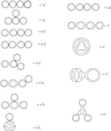
Finally, the third order diagrams are drawn in Figure 6. The combinatorics are tabulated in (2.44). Here the demonstrative example is diagram (b), which is composed of pasting four diagrams, each withh = 2, thush(G) = 4×2 = 8 andC(G) = 24= 16. For F(G), first we have a factor 3!1 from the exponential. Next we have contractions of the form Tr(ΦΦ)3Tr(Φ Φ)Tr(Φ Φ)Tr(Φ Φ); there are
23×4×2 ways of doing this. Thus altogether we haveF(G) = 323eg32 for this diagram. In summary:
diagram (a) (b) (c) (d) (e) (f) (g)
h 8 8 7 7 7 6 6
C(G) 16 16 12 12 12 8 8
F(G) 16eg32 323eg32 64eg22g4 32eg22g4 64ge22g4 128ge2g42 128eg2g42
diagram (h) (i) (j) (k) (l) (m)
h 6 6 5 5 5 5
C(G) 8 9 5 5 5 5
F(G) 32eg2g24 64ge2g42 128g43 323g43 64g34 2563 g34
(2.44)
2.5.4 Obtaining the Effective Action
Now to the highlight of our calculation. From tables (2.42), (2.43), and (2.44) we can readily compute the effective glueball superpotential and free energy. We do so by summing the factors, with the appropriate powers for S, in accordance with (2.39,2.40).
We obtain, up to four-loop order,
F0 =
X
G=all diagrams
F(G)Sh(G)
= (2g4+eg2S)S3−2(9g42+ 8g4eg2S+ 2eg22S2)S4
+ 16 3 (54g
3
4 + 66g42eg2S+ 30g4eg22S2+ 5eg32S3)S5+· · ·, (2.45)
and subsequently,
Wef f = −N S(log(S/Λ2)−1) +
X
G=all diagrams
~g 2
3
(a)
~g 2
3
(b)
g4~g2
x x x (d) 2
g4~g2
x x
x
(e)
2
g4~g2
x x
x 2
(f)
g4~g2
x
x x
2
(g)
g4~g2
x x x (c)
2
g4~g2
x
x x 2
(h)
g4~g2
x x x 2
(i)
g4
x x x (j) 3
g4
x
x x
(k) 3
g4
x
x x (m) 3
g4
x
x
x (l)
3
x x x
x
[image:19.612.92.514.76.571.2]x x
Figure 6: All four-loop primitive and pasting diagrams. The vertices have been marked with a cross.
= −N S(log(S/Λ2)−1) + (6g4+ 4ge2N)N S2−(72g42+ 96g4eg2N + 32eg22N2)N S3
+20
3 (6g4+ 4eg2N)
3N S4+
· · ·. (2.46)
2.6 Multiple Traces, Pasted Diagrams and Nonlocality
Above we found that the only diagrams that contribute to the effective superpotential have zero momentum flowing though the double-trace vertex. Now observe that the double-trace term in the tree-level action can be written in momentum space as:
V =
Z
d4xTr(Φ2(x))Tr(Φ2(x)) =
Z
d4p1d4p2d4p3d4p4Tr(Φ(p1)Φ(p2))Tr(Φ(p3)Φ(p4))δ(p1+p2+p3+p4). (2.47)
Since no momentum flows through the double-trace vertices contributing to the superpotential, the delta function momentum constraint factorizes in our pasted diagrams as
δ(p1+p2+p3+p4)∼δ(p1+p2)δ(p3+p4). (2.48)
Therefore for the purposes of computing the superpotential we might as well replace the double-trace term in the action by
e
V =
Z
d4p1d4p2d4p3d4p4Tr(Φ(p1)Φ(p2))Tr(Φ(p3)Φ(p4))δ(p1+p2) δ(p3+p4)
=
Z
d4x d4yTr(Φ2(x))Tr(Φ2(y)). (2.49) The Feynman diagrams of this nonlocal theory include the ones that compute the superpotential in the double-trace, local theory.
This fact suggests that correlation functions of chiral operators are position independent, as described in [5]. Along with cluster decomposition, this position independence leads to the state-ment that correlators of operators in the chiral ring of an N = 1 theory factorize, which we use in the next section to write hTr(Φ2)2i =hTr(Φ2)i2. However it is subtle to establish the precise
equivalence between factorization of chiral operators and the vanishing that we demonstrated of all except the pasted diagrams, which leads in turn to the nonlocal action in (2.49). We leave this potential connection for exploration in future work.
3. The Field Theory Analysis
In this section, we will show that in the confining vacuum the effective superpotential of the field theory discussed in the previous section is
Wef f =NΛ2+ (6N g4+ 4N2eg2)Λ4. (3.1)
After integrating in the glueball superfield and expanding the superpotential in a power series in S, (3.1) can be written
Wef f =−N S(log(S/Λ2)−1)+(6g4+4eg2N)N S2−2(6g4+4eg2N)2N S3+
20
3 (6g4+4eg2N)
3N S4+· · ·.
We shall compare this expression for the low-energy gauge dynamics to the perturbative field theory computations in Sec. 2. The two results, of course, are in concert.
We begin by considering an N = 1 U(N) gauge theory with a single adjoint superfield Φ deformed fromN = 2 by the tree-level superpotential (n < N)
Wtree = nX+1
r=1
grur+ 4eg2u22, (3.3)
where
uk :=
1 kTr(Φ
k). (3.4)
The tree-level superpotential in (3.3) is more general than the one used in (2.23). Here, we allow single-trace terms at arbitrary powers of Φ. We shall specialize to the previous example at the end of our discussion.
3.1 The Classical Vacua
To find the classical vacua, we have to solve the D-term and F-term conditions. The D-term is proportional to Tr[Φ,Φ]¯ 2which is zero if Φ is diagonal. Let the diagonal entries bexi, i= 1, . . . , N.
We still need to solve the F-term condition. In terms of the xi, the tree-level superpotential is
W = n+1 X r=1 gr r N X i=1
xri +ge2
N X
i=1
x2i
!2
. (3.5)
From this, the F-flatness condition reads: 0 = ∂W
∂xk
=
n+1
X
r=1
grxrk−1+ 4eg2xk N X
i=1
x2i
!
, k= 1, ..., N. (3.6) This is certainly different from the case without the double-trace term, where the F-term equations for differentxks decouple. Here, the eigenvalues interact with each other even at the classical level.
To solve the (3.6), which may be recast as 1
xk n+1
X
r=1
grxrk−1 =−4eg2
N X
i=1
x2i
!
, (3.7)
we take the RHS of (3.7)
C := 4eg2
N X
i=1
x2i
!
, (3.8)
as an unknown constant for all N F-terms. This gives
n+1
X
r=1
grxrk−1+Cxk= 0 ∀ k. (3.9)
As the F-terms are order npolynomials inx, we should generically expectnsolutions for each eigenvalue xk. The eigenvalues are the roots of the polynomial
0 =
n+1
X
r=1
grxrk−1≡gn+1
n Y
i=1
(x−ai). (3.10)
IfNi of the eigenvalues are located at ai, where PiNi =N, the unbroken gauge symmetry is
U(N)→
n Y
i=1
U(Ni). (3.11)
Asais are a function of C, we need to impose the additional consistency condition that
4eg2
n X
j=1
Ni2a2i =C. (3.12)
To simplify the discussion, we henceforth focus on the special case where all of the xis have
the same value. TheSU(N) part of the gauge group is unbroken, and will confine in the infrared.
3.2 The Exact Superpotential in the Confining Vacuum
We now proceed to find the exact superpotential in this confining vacuum [27]. Let us recall the general philosophy of the method (seee.g., [29], whose notations we adopt, for a recent discussion). A generic point in the moduli space of the U(N) N = 2 theory will be lifted by the addition of the the general superpotential (3.3). The points which are not lifted are precisely where at least N −nmutually local monopoles become massless. This can be seen from the following argument. The gauge group in theN = 1 theory is broken down toQni=1U(Ni), and the SU(Ni) factors each
confine. We expect condensation of Ni−1 magnetic monopoles in each of these SU(Ni) factors
and a total of N −n condensed magnetic monopoles. These monopoles condense at the points on the N = 2 moduli space where N −n mutually local monopoles become massless. These are precisely the points which are not lifted by addition of the superpotential. These considerations are equivalent to the requirement that the corresponding Seiberg-Witten curve has the factorization
PN(x, u)2−4Λ2N =HN−n(x)2F2n(x), (3.13)
wherePN(x, u) is an orderN polynomial inx with coefficients determined by the (vevs of) theuk,
Λ is an ultraviolet cut-off, and H and F are, respectively, orderN −n and 2npolynomials inx. TheN−ndouble roots placeN−nconditions on the original variablesuk. We can parametrize
all the huki by n independent variables αj. In other words, the αjs then correspond to massless
fields in the low-energy effective theory. If we know the exact effective action for these fields, to find the vacua, we simply minimize Sef f. Furthermore, substituting huki back into the effective
action gives the action for the vacua.
non-perturbative effects are captured in the Seiberg-Witten curve analysis discussed above. Then, we need to minimize
Wexact=
nX+1
r=1
grhuri+ 4ge2hu22i. (3.14)
In general the factorization problem is hard to solve [30], but for the confining vacuum where all N−1 monopoles have condensed, there is a general solution given by Chebyshev polynomials.2 In our case, we have the solution
up =
N p
[p/2]
X
q=0
Cp2qC2qqΛ2qzp−2q, (3.15)
z= u1
N, C
p n:= n p ! = n!
p!(n−p)!. (3.16) Notice that in (3.15), there is one free parameterz which is the field left upon condensation. Now we put it into the superpotential
W =
n+1
X
r=1
grur(z,Λ) + 4eg2u2(z,Λ)2, (3.17)
solve and back-substitute z from ∂W/∂z = 0 to obtain the effective superpotentialWef f. Notice
that in the above result, we have used
hu22i=hu2i2. (3.18)
This is true becauseu2 is a chiral field, and cluster decomposition in the field theory lets us factor
the correlation functions of operators in the chiral ring [5].
Although the above procedure findsWef f, it is not the best form to compare with our previous
results because there is no gluino condensate S. To make the comparison, we need to “integrate in” [31] the glueball superfield as in [29].
The integrating in procedure is as follows (here we use the single-trace superpotential as an illustrative example of the technique).
• We set ∆ := Λ2, and use the equation N S = ∆∂W
∂∆ =N
n+1
X
r=2
gr
[p/2]
X
q=1
q pC
2q
p C2qqzp−2q∆q (3.19)
to solve for ∆ in terms of S.
• Next, we findz by solving 0 = ∂W
∂z =
n+1
X
r=1
gr
[p/2]
X
q=0
p−2q p C
2q
p C2qqzp−2q−1∆q. (3.20)
2This was worked out first by Douglas and Shenker [32], but here we use the results and nomenclature of Ferrari
• Now the effective action for the glueball superfieldS can be written as WS(S, g,Λ) =−Slog
∆ Λ2
N
+Wtree(S, g,Λ), (3.21)
which will reproduce the result ∂
∂SWS(S,Λ
2, g) =−ln(∆/Λ2)N. (3.22)
3.3 An Explicit Example
Let us work out the double-trace example that we are interested in solving. The superpotential is W =g2u2+ 4g4u4+ 4eg2u22, (3.23)
(later, we can set g2 =m= 1). Using
u2 =
N 2 [z
2+ 2Λ2], (3.24)
u4 = N
4 [z
4+ 12Λ2z2+ 6Λ4], (3.25)
from (3.15), we obtain
W =N z2[g2 2 +g4z
2+ 12g
4Λ2+ 4Neg2Λ2+Neg2z2] (3.26)
+NΛ2[g2+ 6g4Λ2+ 4Neg2Λ2].
From this we have following equations by setting Λ2 = ∆:
S = ∆[g2+ (12g4+ 4Neg2)z2+ (12g4+ 8Neg2)∆], (3.27)
0 = ∂W
∂z =z[g2+z
2(4g
4+ 4Neg2) + 2∆(12g4+ 4Neg2)]. (3.28)
We solvez= 0:
∆ = −g2+
p
g22+ 4S(12g4+ 8Neg2)
2(12g4+ 8Neg2)
. (3.29)
The effective action withS integrated in is3 Wef f =Slog
Λ2 ∆
N
+N∆[g2+ ∆(6g4+ 4Neg2)], (3.30)
which will be the one used in comparison to our previous results. After minimizing this action, we find
Wz=0=NΛ2[g2+ 6g4Λ2+ 4Neg2Λ2], (3.31) 3Notice that in both formula (3.29) and (3.30), g
4 and eg2 combine together asg4+ 2
N
3 eg2. So if we shiftg4 to
g4+2
N
which is the promised result of (3.1). Setting g2 = 1, expanding (3.29) in powers of S, and
substituting into (3.30), we get the second formula (3.2) from the beginning of this section: Wef f =−N S(log(S/Λ2)−1)+(6g4+4eg2N)N S2−2(6g4+4eg2N)2N S3+
20
3 (6g4+4eg2N)
3N S4+· · ·.
(3.32) Crucial in matching the result of this calculation with the perturbative analysis in the previous section is the assumption of factorization hu2
2i = hu2i2. This is equivalent to the vanishing the
pinching diagrams in the perturbative analysis.
4. The Matrix Model
In Sec. 2 we demonstrated that the explicit field theory computation of the effective superpotential localizes to a certain sum of matrix diagrams. All of these diagrams are constructed by pasting planar single-trace diagrams together with double-trace vertices in such a way that no additional momentum loops are created. By examining the scaling of these diagrams withN in (2.39) we also observed that these are precisely the diagrams that would survive the large-M limit of a U(M) bosonic Matrix model with a potential
V(Φ) =g2Tr(Φ2) +g4Tr(Φ4) + e
g2
MTr(Φ
2)Tr(Φ2). (4.1)
The extra factor of 1/M multiplyingeg2, in comparison with the field theory tree-level superpotential
(1.1) is necessary for a well-defined ’t Hooft large-M limit. This is because each trace, being a sum of eigenvalues, will give a term proportional to M. So to prevent the double-trace term from completely dominating the large-M limit we must divide by an extra factor of M. Fortunately, this a well known model and was solved more than a decade ago [22, 33]. Below we will review this solution, compare its results to our field theory calculations, and then generalize to other multi-trace deformations.
4.1 The Mean-Field Method
The basic observation, following [22], that allows us to solve the double-trace matrix model (4.1), is that in the large-M limit the effects on a given matrix eigenvalue of all the other eigenvalues can be treated in a mean field approximation. Accordingly we compute the matrix model free energy
F as
exp(−M2F) =
Z
dM2(Φ) exp{−M(1 2Tr(Φ
2) +g
4Tr(Φ4) +eg2
(Tr(Φ2))2
M )}. (4.2)
= Z Y
i
dλiexp{M(−
1 2
X
i
λ2i − g4 M
X
i
λ4i − ge2 M2(
X
i
λi)2) +X
i6=j
log|λi−λj|}
as mentioned earlier, we should really consider GL(M,C) matrices though the techniques hold
equally). We have introduced an extra factor ofM in the exponent on the right hand side of (4.2) by rescaling the fields and couplings in (4.1) in accordance with the conventions of [22].
The density of eigenvalues
ρ(λ) := 1 M
M X
i=1
δ(λ−λi) (4.3)
becomes continuous in an interval (−2a,2a) whenM goes to infinity in the planar limit for some a ∈ R+. Here the interval is symmetric around zero since our model is an even function. The
normalization condition for eigenvalue density is
Z 2a
−2a
dλρ(λ) = 1 . (4.4)
We can rewrite (4.2) in terms of the eigenvalue density in the continuum limit as exp(−M2F) =
Z YM
i=1
dλiexp{−M2( Z 2a
−2a
dλρ(λ)(1 2λ
2+g
4λ4) (4.5)
+ge2(
Z 2a
−2a
dλρ(λ)λ2)2−
Z 2a
−2a Z 2a
−2a
dλdµρ(λ)ρ(µ) ln|λ−µ|)} . Then the saddle point equation is
1
2λ+ 2g4λ
3+ 2
e
g2cλ=P
Z 2a
−2a
dµ ρ(µ)
λ−µ, (4.6)
wherec is the second moment
c:=
Z 2a
−2a
dλρ(λ)λ2 (4.7)
and P means principal value integration.
The effect of the double-trace is to modify the coefficient ofλin the saddle point equation. We can determine the numbercself-consistently by (4.7). The solution ofρ(λ) to (4.6) can be obtained by standard matrix model techniques by introducing a resolvent. The answer is
ρ(λ) = 1 π
1
2 + 2ge2c+ 4g4a
2+ 2g 4λ2
p
4a2−λ. (4.8)
Plugging the solution into (4.4) and (4.7) we obtain two equations that determine the parameters aand c:
a2(1 + 4eg2c) = 1−12g4a4, (4.9)
16g4eg2a8+ (12g4 + 4eg2)a4+a2−1 = 0. (4.10)
Substituting these expressions into (4.5) gives us the free energy in the planar limit M → ∞ as:
F =
Z 2a
−2a
dλρ(λ)(1 2λ
2+g
4λ4) +eg2c2−
Z Z 2a
−2a
dλdµρ(λ)ρ(µ) ln|λ−µ|.
One obtains
F(g4,eg2)− F(0,0) =
1 4(a
2−1) + (6g
4a4+a2−2)g4a4−
1 2log(a
2) . (4.12)
Equation (4.12) together with (4.10) give the planar free energy. We can also expand the free energy in powers of the couplings, by using (4.10) to solve for a2 perturbatively
a2 = 1−(12g4+ 4eg2) + (288g42+ 176g4eg2+ 32eg22) (4.13) −(8640g43+ 7488g42eg2+ 2496g4eg22+ 320eg32) +· · ·.
Plugging this back into (4.12) we find the free energy as a perturbative series
F0=F(g4,eg2)− F(0,0) = 2g4+ge2−2(9g24+ 8g4ge2+ 2eg22) +
16 3 (54g
3
4+ 66g24eg2+ 30g4ge22+ 5eg23) +· · ·.
(4.14) Comparing with (2.45) we see that F reproduces the explicit computation of the generating function of “planar pasted” field theory diagrams in Sec. 2.5. In matching the two we have to restore the proper powers of the glueballS into (4.14). First recall that to keep the relevant diagrams in the matrix model, we have inserted M1 to the double-trace term in (4.1). Therefore to compare with (2.45), we need to rescale eg2 in (4.14) to eg2M ≡eg2S where we have effectively identified the
glueball S in the field theory withM in the matrix model. In addition, we should re-insert powers ofM into (4.14) by loop counting. The first two terms in (4.14) have three index loops so we need to multiply them by M3 ≡ S3. The third term has four index loops and fourth term, five and hence we respectively need factors of S4 and S5. With these factors correctly placed into (4.14),
we recover (2.45) completely.
This verifies our claim that the diagrams surviving the large-M limit of the matrix model (4.1) are precisely the graphs that contribute to effective action of the field theory with the tree-level superpotential (1.1). Nevertheless, as we have already discussed in Sec. 2.4 we cannot compute the effective superpotential of the field theory Wef f(S) by taking a derivative ∂F0/∂S, because the
combinatorial factors will not agree. In this way the double-trace theories differ in a significant way from the single-trace models discussed by Dijkgraaf and Vafa [3]. We can pose the challenge of finding the field theories who effective superpotential is computed by the Matrix model (4.12).
4.2 Generalized Multi-Trace Deformations
In fact the mean field techniques of the previous subsection can be generalized to solve the general multi-trace model. Below we illustrate this by solving the general quartic Matrix model; as discussed above, it is an interesting challenge to find a find a field theory whose effective superpotential these models compute.
Specifically, let us consider the Lagrangian
L=g2Tr(Φ)2+µ(Tr(Φ))2+ν1(TrΦ)2(Tr(Φ2)) +ν2(TrΦ)4+ 2ν3(TrΦ)(Tr(Φ3)), (4.15)
The one-matrix model partition function ZM =
Z
[Dλ] exp
−M2
L − Z 1 0 dx Z 1 0
dy log|λ(x)−λ(y)|
, (4.16) gives the saddle point equation
4g4λ3+ 6ν3c1λ2+ 2(g2+ 2eg2c2+ν1c21)λ+ 2(µc1+ν1c1c2+ 2ν2c31+ν3c3) = 2P
Z 2b
−2a
dτ u(τ)
λ−τ, (4.17) where the moments ck are defined as
ck = Z 2b
−2a
dτ u(τ)τk, c0 =
Z 2b
−2a
dτ u(τ) = 1. (4.18)
Note that we have introduced the separate upper and lower cut parametersaandbas opposed to the standard symmetric treatment becauseu(λ) is not of explicit parity (such asymmetric examples have also been considered in [26]). When a = b one can recast (4.17) into a Fredholm integral equation of the first kind and Cauchy type, which affords a general solution as follows [36]
P1 π
Z a
−a
u(t)dt
t−x =−v(x)⇒u(x) = 1 π
Z a
−a r
a2−t2
a2−x2
!
v(t)dt t−x +
C
√
a2−x2 (4.19)
for some constant C. Whena6=bwe can use the ansatz: u(λ) = 1
π(Aλ
2+Bλ+C)p(2a+λ)(2b−λ) (4.20)
with the constants matching the coefficients in the LHS of (4.17) as
2A = 2g4, (4.21)
2aA−2Ab+ 2B = 3ν3c1,
−a2A−2a A b−A b2+ 2a B−2b B+ 2C = g2+ 2eg2c2+ν1c21,
a3A+a2A b−a A b2−A b3−a2B−2a b B−b2B+ 2a C−2b C = µc1+ν1c1c2+ 2ν2c31+ν3c3.
We see a well-behaved u(λ) which is zero at the end-points and vanishes outside the support (−2a,2b).
We now need to check the consistency of our mean-field method. This simply means the follow-ing. Considering the definition ofci in (4.18), the definitions (4.21) actually constitute a system of
equations forA, B, C, a, b because each ci on the RHS, through (4.18), depend on A, B, C, a, b. To
(4.21) we must append one more normalization condition, thatc0=R−2b2au(λ)dλ= 1. Therefore we
5. Linearizing Traces: How To Identify the Glueball?
In previous sections we showed that the field theory computation of the effective superpotential of a double-trace theory as a function of the glueball S localized to summing Matrix diagrams. In the end, the only the “pasted” diagrams that contributed, namely certain tree-like graphs obtained by pasting together planar single-trace graphs with double-trace vertices in such a way that no momentum flows through the latter. After verifying the result via the N = 2 Seiberg-Witten solution, we demonstrated that the sum of these diagrams given as a series in (2.39) is not computed by the large M limit of aU(M) Matrix as one would have naturally hoped. Nevertheless, we may wonder if there is some Matrix model that sums the series of pasted diagrams. In this section we take up the challenge of finding such a Matrix model.
Since the authors [4] and [5] have proven that the superpotential of a single-trace gauge theory can be computed from an associated Matrix model, we seek to construct our double-trace theory from another single-trace model. Recall that we are considering the tree-level superpotential
Wtree =
1
2g2Tr(Φ
2) +g
4Tr(Φ4) +eg2(Tr(Φ2))2. (5.1)
Now consider another theory with an additional gauge singlet fieldA Wtree =
1
2(g2+ 4eg2A)Tr(Φ
2) +g
4Tr(Φ4)−eg2A2. (5.2)
It is easy to see that integrating out A in (5.2), which amounts to solving ∂Wtree
∂A = 0 and
back-substituting, produces the double-trace theory (5.1).
The advantage of (5.2) is that it consists purely of single-trace operators. The first two terms will generate an effective potential Wsingle(A, S), as a function of A and the glueball superfield S
(the subscript “single” refers to the fact that this is the superpotential for the model without the double-trace term and with an Adependent mass term). Then
Weff(A, S) =Wsingle(A, S)−eg2A2. (5.3)
The exact superpotential for the glueball superfield S for the double-trace theory then follows by integrating A out, i.e. solving ∂Wsingle
∂A −2eg2A = 0 for A and substituting in (5.3). Since
single-trace theories are directly related to Matrix model we might hope to use this construction with an added auxiliary field A to find an auxiliary Matrix model that sums the pasted diagrams of the double-trace theory.
5.1 Field Theory Computation of Wsingle(A,S) and Pasted Matrix Diagrams
In this section4 we will discuss how the superpotential for the double-trace theory can be computed
in field theory from the linearized model (5.2). First, observe that the superpotential for an adjoint theory with an additional gauge singlet (5.2) localizes to summing matrix integrals, since the arguments of [4] that are reviewed in Sec. 2 go through essentially unchanged. To compute the
effective potential as a function of bothA and the glueballS, we need to sum superspace Feynman diagrams with insertions of bothAandWα, with both of these treated as background fields. Since
we are only interested in contributions to the superpotential, we can restrict ourselves to constant background A. Then it is easy to verify that the entire analysis in Sec. 2 goes through for the theory (5.2), with the double-trace coupling eg2 set to zero and a shift in the mass of the field
Φ, viz g2 → g2 + 4eg2. In particular, the computation of the effective superpotentialWsingle(A, S)
localizes to summing matrix diagrams and there is some free energy Fsingle in terms of which
Wsingle =N ∂Fsingle(S, A)/∂S.
Let us verify that this procedure will yield the correct double-trace result when we integrate A out. Making theg2 → g2+ 4eg2 witheg2 = 0 in the known single-trace result (3.30) and (3.29), we
find the effective superpotential
Wsingle(A, S) =N Slog(
Λ2
∆) +N∆((g2+ 4eg2A) + 6g4∆), (5.4) where ∆ is determined by the quadratic equation
12g4∆2+ (g2+ 4eg2A)∆ =S. (5.5)
Now we can integrate Aout and obtain the superpotential for the glueball superfield S. We solve ∂Weff/∂A=∂Wsingle/∂A−2eg2A= 0 forA. This is a simple calculation from (5.4), (5.5):
∂
∂AWsingle(∆(S, A), S, A) =
∂Wsingle
∂A + ∂∆ ∂A
∂Wsingle
∂∆ (5.6)
= (g2+ 4eg2A+ 12g4∆−
S ∆)N
∂∆
∂A + 4eg2N∆ = 4ge22N∆,
where in last step we have used (5.5). So the solution to ∂Wsingle/∂A−2eg2A= 0 is
A= 2N∆. (5.7)
PluggingA= 2N∆ into (5.4), (5.5) and (5.3), we find the effective glueball superpotential to be Weff =N Slog(
Λ2
∆) +N∆(g2+ 4eg2N∆ + 6g4∆), (5.8) with ∆ determined by the quadratic equation
(12g4+ 8eg2N)∆2+g2∆ =S. (5.9)
Equations (5.8) and (5.9) are of course the double-trace effective glueball superpotential we com-puted previously in (3.29) and (3.30).
theory with a quartic superpotential, and after doing so, we obtain the superpotentialR d4xd2θ W
with
W =Wconnected planar(S, g2+ 4eg2A, g4)−eg2A2. (5.10)
Next, we should integrate out A. To do so, we write A = A0+A, wheree A0 solves ∂W/∂A = 0.
We see thatW becomes
W =Wconnected planar(S, g2+ 4eg2A0, g4)−eg2A20+c2Ae2+c3Ae3+. . . . (5.11)
What is the meaning of integrating over A? From the diagrammatic point of view,e Aeis the field that allows momentum to flow through theeg2 vertices. All diagrams where such momentum flow is
prohibited are taken into account by the background valueA0. Thus, pickingA0 takes the pasting
process into account, whereas the further integrals overAeshould correspond to pinching diagrams. We already know that these latter diagrams should vanish from our diagrammatic analysis, and therefore we should simply drop all terms involving A. The final answer fore W is thus
W =Wconnected planar(S, g2+ 4eg2A0, g4)−ge2A20. (5.12)
One can also see directly that integrating outAegives no contribution to the superpotential. In the diagrams that one can write down, there will be many loops of A, but there are no vertices thate can absorb any fermionic momentum, and therefore these diagrams do not yield any contribution to the superpotential.
It is an interesting exercise to verify explicitly that (5.12) is a generating diagram for pasted diagrams (which are all tree graphs), made out of building blocks corresponding toWconnected planar.
5.2 Matrix model perspective
Above we argued that the methods of [4] show that above linearization of the double-trace defor-mation via introduction of an auxiliary singlet field A leads to a theory whose superpotential be computed by a matrix model.
First observe that the double-trace matrix model partition function can be linearized in traces by the introduction of an auxiliary parameterA, over which we integrate:
Z = exp(−M2F0double) =
Z
dM2(Φ) exp{−M(1
2g2Tr(Φ
2) +g
4Tr(Φ4) +eg2
(Tr(Φ2))2
M )} (5.13) =
Z
dA dM2(Φ) exp{−M(1
2(g2+ 4ge2A)Tr(Φ
2) +g
4Tr(Φ4)−Meg2A2)}.
This is is Matrix model analog of the statement that the double-trace field theory can be generated by integrating out a gauge singlet. In terms of the free energy of the single-trace matrix model, this can be written as
exp(−M2F0double) =
Z
dAexp(−M2F0single+M2eg2A2). (5.14)
Hence to obtain the free energy of the double-trace matrix model, we need to solve the equation
∂F0single(A,S)
∂A −2eg2A = 0 for A and substitute in F0double = F single