Influence of laser-drive parameters on annular fast electron transport in silicon

Influence of Laser-Drive Parameters on Annular Fast

Electron Transport in Silicon

D. A. MacLellan

, D. C. Carroll

, R. J. Gray

, A. P. L. Robinson

, M. P.

Desjarlais

_{, D. Neely}

_{, and P. McKenna}

1

_{Department of Physics, SUPA, University of Strathclyde, Glasgow G4 0NG, UK}

_{Central Laser Facility, STFC Rutherford Appleton Laboratory, Oxfordshire}

OX11 0QX, UK

3

_{Sandia National Laboratories, P.O. Box 5800, Albuquerque, New Mexico 87185,}

USA

December 20, 2013

Corresponding author: Paul McKenna, Department of Physics, SUPA,

University of Strathclyde, Glasgow G4 0NG, United Kingdom. E-mail:

Abstract

Three dimensional hybrid particle-in-cell (PIC) simulations are used to investigate the

sensitivity of annular fast electron transport patterns in silicon to the properties of the

drive laser pulse. It is found that the annular transport, which is induced by self-generated

resistive magnetic fields, is particularly sensitive to the peak laser pulse intensity. The

radius of the annular fast electron distribution can be varied by changing the drive laser

pulse properties, and in particular the focal spot size. An ability to optically ‘tune’ the

properties of an annular fast electron transport pattern could have important implications

for the development of advanced ignition schemes and for tailoring the properties of beams

1

Introduction

The large currents of relativistic (fast) electrons generated in the interaction of an ultraintense

laser pulse with a solid can be used to drive the formation of strong fields and for heating

applications, often at significant distances (hundreds of microns) from the source. Understanding

the transport physics of these electrons in solids is therefore important for applications such as

the fast ignition approach to inertial confinement fusion [1] and for tailoring the properties of

beams of sheath-accelerated ions [2].

In recent years, attention has focused on the role of target electric resistivity in defining the

properties of fast electron transport, both in terms of the different transport patterns in metals

and insulators (see for example [3, 4, 5]), and in the possible use of self-generated resistive

magnetic fields to control fast electron transport. As the fast electron population is accelerated

into the target it draws a balancing cold return current, spatially overlapped with it and moving

in the opposite direction, to satisfy the overall charge neutrality requirement [6]. If the fast

electron current density is designated as jf and the cold return current density as jr then

jf +jr ≈ 0 [7]. From Ohm’s law, the self-generated electric field is E = −ηjf, which when

combined with Faradays law enables the self-generated magnetic fieldBto be written as ∂_∂tB =

η∇ ×jf +∇η×jf where η is the target resistivity and t is time. The first term on the right

hand side of this equation (η∇ ×jf) generates a magnetic field which pushes fast electrons into

regions of higher current density, while the action of the second term (∇η×jf) is to push fast

electrons into regions of higher resistivity. The resulting magnetic field strength and growth

rate can be significant. Growth rates of∼1014 _Ts−1_{are produced in typical intense laser-solid}

interactions i.e. approximately 200 T in 1 ps. Fields of this magnitude have a strong effect

on the propagation of multi-MeV electrons, and give rise to effects such as beam pinching or

collimation [8], hollowing [9] and resistive instability-driven filamentation [10].

Schemes involving structured targets have been explored both experimentally [11, 12] and

numerically [13] in an effort to use resistive gradients formed at the boundary between two

different materials to induce magnetic field growth within solids, with the aim of collimating the

fast electron beam. An extension of this layered target approach has been proposed to produce a

‘magnetic switch-yard’ scheme for controlling fast electron transport in advanced fusion targets

[14]. In other work a technique for optically controlling the divergence of the electron beam by

using double laser pulse drive has been demonstrated [15].

Recently we have shown that the resistivity of the solid at relatively low temperatures (eV

to tens of eV regime) can have a defining influence on the properties of fast electron transport

the resistivity evolution of the target and the subsequent onset of resistive fast electron beam

filamentation was demonstrated [16]. It was shown that the shape of the resistivity-temperature

profile of the target material plays a key role in defining the beam transport pattern. An annular

beam profile was demonstrated in silicon, arising due to a dip in resistivity at a few eV [17].

The ability to fundamentally change the beam transport pattern from a Gaussian-like to an

annular fast electron beam profile by controlling the resistively generated magnetic fields could

have important consequences for applications. Alfv´en showed that compared to a uniform beam,

a higher current can be transported in an annular beam [18]. The Alfv´en limit increases by a

factor of r/δr, where r is the radius of the beam and δr is the width of the annulus. Davies [19] developed the idea by proposing schemes directly applicable to fast ignition, and Hatchett

et al [20] discusses the advantages of using annular beams to reduce the energy requirements of

the ignition drive beam. Annular fast electron beam transport in a solid can also be used to

produce an annular beam of sheath-accelerated ions [17]. Temporal et al [21] proposes the use

of an annular proton beam in combination with a second uniform proton beam to reduce the

total energy required for ignition by a factor of almost two compared to a single uniform proton

beam. Thus understanding and controlling the formation and subsequent evolution of annular

fast electron beam transport is not only of fundamental interest, but may also have important

implications for applications of intense laser-solid interactions.

In this paper, the sensitivity of annular fast electron beam transport to the parameters of

the drive laser pulse is investigated numerically via 3D hybrid-PIC simulations. Changes to the

size of the ring and the density of the electrons forming it are quantified as a function of laser

pulse energy, duration and focal spot radius, and explained in terms of the effects on the resistive

magnetic fields.

2

Modelling

The particle-based 3D-hybrid code ZEPHYROS [11, 14], in which the fast electrons are described

using a PIC algorithm while the background plasma is treated as a fluid [22, 23], is used. A 200

µm ×400 µm ×400 µm simulation grid was used, with a cell resolution of ∆X = ∆Y = ∆Z = 1 µm. As with many other hybrid-PIC codes, the fast electron source is not calculated self-consistently. The properties of the electron beam at the source are defined based on previous

theory, experiment and PIC simulation studies of fast electron generation, and the electrons

are introduced or injected into the computational grid in a ‘laser-spot’ profile region. The

electron source is centred at [X, Y, Z] = [0, 0, 0], with a transverse intensity profile determined

by I = αILexp(−_rr

is the peak laser intensity and α is the fraction of laser energy converted to fast electrons (set to 0.3). The electron pulse has a top-hat temporal profile. The fast electrons propagate

in the X-direction with an exponential energy distribution (of the form exp(−E

Tf)), where E is the electron kinetic energy and the mean temperature Tf scales ponderomotively (kBTf =

0.511[(1 + 0.73I18λ2µm)1/2−1] MeV, whereI18is the peak laser intensity in units of 1018Wcm−2 and λµm is the laser wavelength in microns [24]). The electrons are injected with a uniform

angular distribution over a cone subtended by a half-angle of 50◦[25] and in all cases the initial

target temperature is set equal to 1 eV.

Although the fast electron source parameters, as defined by the percentage of the laser energy

absorbed by the electrons and their injection angle and distribution, are expected to vary with

the properties of the laser pulse, the precise nature of these dependencies are still not well

understood and are the subject of ongoing work. Therefore, as this investigation focuses on the

transport pattern of the fast electron beam within the target, the source properties are kept

constant throughout.

100 101 102 103

10−7 10−6

Temperature [eV]

Resistivity [

Ω

m]

(a) (b) (c)

Figure 1: (a) Electrical resistivity of silicon as a function of target temperature, based onab initio

QMD calculations coupled with the Kubo-Greenwood equation [17]. (b, c) Example hybrid-PIC

simulation results showing 2D maps (1400 fs into the simulation) of (b) the target temperature

in eV, with selected isothermal contours, and (c) the corresponding magnetic flux density (BZ

component in Tesla), showing a collimating component which acts to limit the divergence of the

beam and a hollowing component arising from a reversal in the magnetic field direction inside

the edge of the beam.

The silicon resistivity-temperature profile used, presented in figure 1(a), is based on a

quan-tum molecular dynamics (QMD) Kubo-Greenwood calculation [26, 27], as discussed in MacLellan

in the resistivity gradient near the edges of the fast electron beam, where the target is heated

to relatively low temperatures. An example 2D temperature map from the simulations (for IL

= 5×1020_Wcm−2_{; E}

L = 192 J;τL = 1 ps and rL = 3.5µm) is shown in figure 1(b) and the

corresponding 2D map of magnetic flux density is shown in 1(c), (both sampled after 1400 fs).

This reversal in the resistivity gradient leads to a reversal in the direction of the self-generated

resistive magnetic field, via the∇η×jf term. The combination of the collimating effect of the

azimuthal magnetic field enveloping the beam (the collimating component) and the reversed

magnetic field just inside the edge of the beam (the hollowing component) drive a localized

increase in the fast electron beam current density in an annular profile. If the ring is of sufficient

size and contains a large enough fraction of the total electron current, the transport pattern is

maintained and even reinforced as the electrons propagate across the remainder of the target.

The reinforcement occurs due to the local increase in resistive heating arising from the increase

in jf (resistive heating scales as j2f) which drives a local increase in resistivity and thus larger

resistivity gradients and azimuthal B-fields surrounding the annulus.

3

Simulation Results

We begin by defining two parameters to quantify annular transport in the simulation results.

These are: (1) the inner radius of the annulus at the end of the simulation box, i.e. at X =

200µm(this is defined as the ratio at which the electron density increases by a factor of 5 with respect to the axial density); and, (2) the ratio of the electron densities in the annulus to the

axial position ([200,0,0]), again at the end of the simulation box. These quantities effectively

measure the size of the ring and the annulus-to-axial contrast ratio.

To investigate the sensitivity of these parameters to the drive laser pulse parameters, three

series of simulation scans were performed, as follows: A) variation of laser pulse energy,EL in

the range 78 - 385 J, for fixed focal spot radiusrL= 3.5µm and fixed laser pulse durationτL =

1 ps; B) variation ofrL in the range 2.5 - 5.5µm, for fixedEL = 192 J andτL = 1 ps; and, C)

variation ofτLin the range 0.5 - 2.5 ps, for fixedEL= 192 J andrL= 3.5µm. These parameter

ranges were chosen such that the peak laser pulse intensity,IL, was varied in the range 2×1020

- 1×1021 Wcm−2 for all three scans.

Figure 2 presents the results from these simulations. The fast electron density in the [X,

Y] mid-plane is shown, at an example time of τL + 0.4 ps - this time is chosen such that the

full population of electrons has been initiated in the simulation and has propagated at least 100

by reflection at the target rear side, occurs in the simulation (fast electron refluxing has been

previously shown to perturb the resistive magnetic field structure within solids [28]). Scan A is

presented in the top row (figure 2(a - e)), B in the middle row (figure 2(f - j)), and C in the

bottom row (figure 2(k - o)). The corresponding simulation outputs for the [Y, Z] rear-plane

snapshots are displayed in figure 3.

2×1020 _Wcm−2 _2.5×1020_Wcm−2 _3.3×1020 _Wcm−2 _5×1020 _Wcm−2 _1×1021 _Wcm−2

τL = 1 ps

rL = 3.5µm

EL = 192 J

τL = 1 ps

EL = 192 J

rL = 3.5µm

A

B

C

(a)EL= 78 J (b)EL= 96 J (c)EL= 128 J (d)EL= 192 J (e)EL= 384 J

(f)rL= 5.5µm (g)rL= 5µm (h)rL= 4.3µm (i)rL= 3.5µm (j)rL= 2.5µm

(k)τL= 2.5 ps (l)τL= 2 ps (m)τL= 1.5 ps (n)τL= 1 ps (o)τL= 0.5 ps

Figure 2: 2D maps of the fast electron beam density (log10), in units of m−3_{, in the [X-Y]}

mid-plane of the simulation, for three laser pulse parameter scans: (a-e) variation of EL (top

row); (f-j) variation of rL (middle row); (k-o) variation ofτL (bottom row). The value of the

2×1020 Wcm−2 2.5×1020 Wcm−2 3.3×1020 Wcm−2 5×1020Wcm−2 1×1021Wcm−2

τL = 1 ps

rL = 3.5µm

EL = 192 J

τL = 1 ps

EL = 192 J

rL = 3.5µm

A

B

C

(a)EL= 78 J (b)EL= 96 J (c)EL= 128 J (d)EL= 192 J (e)EL= 385 J

(f)rL= 5.5µm (g)rL= 5µm (h)rL= 4.3µm (i)rL= 3.5µm (j)rL= 2.5µm

(k)τL= 2.5 ps (l)τL= 2 ps (m)τL= 1.5 ps (n)τL= 1 ps (o)τL= 0.5 ps

Figure 3: Same as figure 2, but for the rear surface [Y-Z] plane

In scan A, we find that increasing the energy from 78 J to 385 J, which effectively increases

the current of electrons, results in an increase in the overall divergence of the electron beam and

thus an increase in the radius of the annular feature. By contrast, when increasing the intensity

over the same range by decreasing the focal spot radius fromrL= 5.54µm to 2.48µm, scan B,

the increase in both the overall beam divergence and the radius of the ring is smaller. Note that

the fixed laser pulse energy in combination with the increasing laser intensity means that fewer

electrons are injected as the focal spot radius is decreased, producing the beam density decrease

observed in figure 2(f - j). This influences the target temperature and resistivity evolution,

and subsequent electron transport properties, as will be explained later. In scan C, significant

changes in the beam transport are found for variation of the pulse duration. AsτL is increased

over the range 1 ps to 2.5 ps, the overall beam divergence and radius of the annular structure

are found to decrease, effectively leading to more uniform beam transport for the longer pulse

structure and a significant increase in the overall fast electron beam divergence which, as will

be discussed later, is a result of a reduction in the magnetic field strength.

To examine these trends more closely, the rear-surface simulation outputs from figure 3 are

analysed to quantify the variation of the size of the annulus and the relative density of electrons

contained within it, as a function of IL for each of the three scans. The radius of the annular

structure is defined as the distance from the centre of the rear-surface simulation grid (i.e. at [Y,

Z] = [0, 0]) to the inner annulus of the ring structure, and the results are shown in figure 4(a).

Note that the 1021Wcm−2point in scan C (τL = 0.5 ps) is excluded as a clear ring profile is not

observed for this case. Figure 4(b) shows the ratio of the fast electron density in the annulus

(peak density) to the density of the centre of the beam, [Y, Z] = [0, 0].

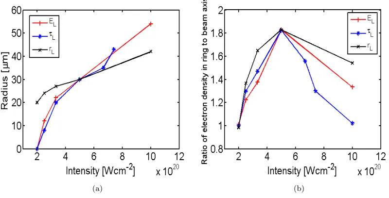
(a) (b)

Figure 4: (a) Inner radius of the annulus at the target rear surface as a function ofIL, for the

three parameter scans shown in figure 2 and figure 3. (b) Ratio of the fast electron density

in the annulus to the density on-axis (i.e. at [200,0,0]) as a function of IL, for the same three

parameter scans.

Overall effect of laser intensity

Considering first the variation of the size of the ring, we find that the radius increases with

increasing peak laser intensity for all three scans. This is due to the increase in the overall

divergence of the fast electron beam with increasingIL. Since the magnetic field reversal driving

of a few eV), the radius of the ring is, to first order, defined by the overall beam divergence.

The divergence in turn depends on the angular distribution of the electrons at the source (which

is fixed in our simulations) and the strength of the collimating magnetic field. The field is

strongest within the first few tens of microns from the front surface where the current density

is highest and can be approximated as a cylinder - hollowing is not seeded until a depth of

∼ 40µm (as shown in figure 1(c)). The resistive azimuthal magnetic field around a uniform cylindrical electron beam of radiusrf can be estimated as ∂_∂tB =ηjf/rf, where the fast electron

current is given byjf =If/Tf, in which If is the fast electron beam intensity [8]. The inverse

dependence of the strength of the collimating magnetic field on the fast electron energyTf is due

to the decrease in jf as Tf is increased. Tf scales ponderomotively with the square root of the

laser intensity, and hence as the peak laser intensity increases the magnetic field strength and

therefore it’s global pinching effect on the fast electron beam decreases, increasing the overall

beam divergence. Thus the radius of the ring induced by the hollowing component of the field

formed near the edge of the beam increases with IL. We note that the laser-to-electron energy

conversion efficiency is likely to change with IL, which will also effect magnetic field growth.

However the precise dependencies of the energy coupling efficiency on each of the laser pulse

parameters are not well enough known to factor this into the study and therefore, as highlighted

in section 2, this parameter is fixed.

As shown in figure 4(b), for all three pulse parameter scans the ratio of the electron density

in the annulus to the axial density is highest forIL = 5×1020Wcm−2 (the same result at this

intensity forms part of the simulation set for all three scans). With decreasing laser intensity,

the overall beam divergence and ring radius decreases (due largely to the reduction in Tf, as

discussed above) resulting in a higher beam density on-axis. Although hollowing still occurs

at low IL, the ratio of the beam densities in the annulus to the axial position decreases as

the collimating effect of the magnetic field dominates over the hollowing term for small beam

radii. With increasingIL above 5×1020Wcm−2, the rate of the resistive magnetic field growth

decreases. Therefore, although the beam radius increases, which should enhance the ratio, the

lower magnitude of the hollowing magnetic field and higher Tf results in less electrons being

deflected to form the ring. Since the local jf of the annulus thereby decreases, the rate of

localised resistive heating is lower and so the reinforcing feedback condition discussed above is

Laser focal spot dependence

Although for all three parameter scans, the ring radius increases with IL, it is clear from

fig-ure 4(a) that the scaling with intensity is different when varying the focal spot radius compared

to variation of eitherEL orτL. This difference is accounted for by the size of the electron beam

at source. A decrease inrL has two main effects: (1)jf, and hence B, increases, decreasing the

overall divergence of the beam; and, (2) the radius at which hollowing is seeded decreases. Both

effects influence the radius of the beam annulus downstream, and we consider each in turn:

(1) The magnetic field which defines the overall beam divergence scales inversely withrf, as

discussed above, and is strongest at the source, where jf is highest and defined by the size of

the laser focal spot. Let us consider the simulation result at 5×1020_Wcm−2_{, which is common}

to all three scans, and for which rL = 3.5 µm, as a reference. AsrL is decreased to 2.5 µm

(1×1021 _Wcm−2_{), j}

f at the source, and hence the peak magnetic field strength, is enhanced

by approximately a factor of two. The simulation result shows a reduction in the annulus

radius, corresponding to an overall beam divergence angle reduction of∼36%, compared to the

simulations at the same intensity in scans A and C for whichrL= 3.5µm. Similarly, an increase

in rL from 3.5 µm to 4.3 µm(IL = 3.3×1020 Wcm−2) results in a 50% decrease in jf and B

at the source, which contributes to the∼35% increase in the ring divergence in the simulation results (again compared to the simulations at the same intensity in scans A and C).

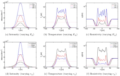
(2) The effect of varyingrL on the radius at which the annular transport pattern is seeded

is explored in figure 5. The transverse intensity profiles of the drive laser pulse are shown in

figure 5(a) and (d) for the energy and focal spot scans (A and B), respectively. For brevity,

scan C is not considered in detail because the results are very similar to A. For each scan,

three example IL are considered: 2×1020 Wcm−2, 5×1020 Wcm−2 and 1×1021 Wcm−2

(displayed as the black, red and blue plots, respectively) and the full width at half maximum

(FWHM) for each is marked. The corresponding target temperature and resulting resistivity

profiles (along the Y-axis) at X = 50 µm (depth at which the annular transport evolves) are shown in figure 5(b) - (c) and figure 5(e) - (f) for scan A and B respectively. The red dotted line

highlights the temperature at 3.5 eV and the corresponding reversal in the resistivity gradient

at the edges of the beam which seeds annular transport [17]. From these plots we see that the

radius at which seeding of the annular transport occurs increases with intensity for scan A (and

C), but decreases slightly with intensity for scan B, due to the change inrL. ForIL= 2×1020

Wcm−2_{, for example, the radius at which annular transport is seeded is∼35% larger in scan B}

than A, due to the larger rL, which contributes to the larger annular profile at the rear of the

(a) Intensity (varyingEL) (b) Temperature (varyingEL) (c) Resistivity (varyingEL)

(d) Intensity (varyingrL) (e) Temperature (varyingrL) (f) Resistivity (varyingrL)

Figure 5: Variation of (a) the laser pulse intensity, (b) the target temperature at X = 50µmand (c) electrical resistivity at X = 50 µm along the Y-axis, all for three example peak intensities (2×1020_Wcm−2_{-black, 5×10}20_Wcm−2_{-red and 1×10}21_Wcm−2_{-blue) obtained by variation of}

EL (values given). (d-f) Same as (a-c), for the same three peak intensities, but for variation of

rL(values given). Dotted lines in (a) and (c) highlight the FWHM of the intensity distributions.

Dotted lines in (b) and (e) mark the important 3.5 eV target temperature, and in (c) and (f)

mark the corresponding turning points in the target resistivity which seeds annular fast electron

beam transport.

Note that the simulation profiles in figure 5 show spikes in target temperature which grow

at the edge of the beam and arise due to the local increase in the beam density (and hence

collisional return current) due to the deflection induced by the magnetic field. As discussed

above and in MacLellanet al [17], this drives a localized increase in resistivity for temperatures

above ∼3.5 eV and hence the region near the edge of the beam remains more resistive than

the centre, which reinforces the annular transport pattern as the beam propagates over the

remainder of the target.

With reference to figure 5(e), it is interesting to note that reducing rL for fixed EL and

τL significantly reduces the overall heating of the target. This occurs because IL and hence

efficiency from laser to electrons), reduces the total number of fast electrons, and hence j2

f

heating. Additionally, we note that there is a general trend of the onset of fast electron beam

filamentation with increasingEL, as manifested in the temperature oscillations across the beam

observed in 5(b). This is a consequence of the increase in background temperature between

∼3.5 eV and∼70 eV, which produces a high resistivity (figure 1), leading to a higher resistive

instability growth rate [16].

Influence of laser pulse duration

To explore why the annular transport pattern is washed out for the τL = 0.5 ps simulation in

scan C, the spatial profile of the resistively generated magnetic field is examined as a function

of τL. Lineouts are extracted along the Y-direction (i.e. transverse, or radial, profile) of the

simulation grid, at the X-axis position to which the magnetic field extends (which changes with

τL). This is defined as the position at which the magnitude of the collimating magnetic field is

reduced by 50%. For the cases shown in figure 6(a), this represents depths of 45µm, 50µm, 55

µm, 60µm and 65µm forτL = 0.5 ps, 1 ps, 1.5 ps, 2 ps and 2.5 ps respectively. The resulting

field profiles are shown in figure 6(a) for radius up to 80µm (i.e. Y = 0 corresponds to the centre of the beam) for each of the five simulations. These plots demonstrate the complex interplay

between pulse duration and the generation of the collimating magnetic field which envelopes

the beam, forcing the electrons towards the axis (positiveBZ in figure 6(a)), and the hollowing

reversed magnetic field which forms just inside the circumference of the beam, driving electrons

outwards (negative BZ in figure 6(a)). Achieving a balance between these opposing azimuthal

(a) (b) (c)

Figure 6: (a) Variation of the self-generated resistive magnetic field as a function of beam radius

(Y-axis) at the penetration depth over which the magnetic field extends: 45µm, 50µm, 55µm, 60 µm and 65µm forτL = 0.5 ps, 1 ps, 1.5 ps, 2 ps and 2.5 ps respectively. (b) Magnitude of

the collimating and hollowing magnetic field components as a function of time for givenτL. (c)

Magnitude of the collimating and hollowing magnetic field components as a function ofτL.

The magnitude and rate of the resistive magnetic field growth depend on both the fast

electron current density and bunch duration (effectively the drive laser-pulse duration) [6].

Fig-ure 6(a) shows example profiles of the magnetic field, exhibiting both the collimating component

and the oppositely-directed hollowing component, for given τL. We find that the amplitude of

both magnetic field components increases with pulse duration, as a consequence of the longer

duration over which the field grows [22], and generally that the differences between the

mag-nitude of the components decreases. This is observed in figure 6(b) which shows the temporal

evolution of both magnetic field components for three example τL, and figure 6(c) showing the

magnitude of both components as a function of pulse duration. The greatest difference between

the two components is observed forτL= 1 ps, which explains the resulting strong annular

trans-port patterns. With increasing pulse duration the difference decreases, as the collimating field

becomes more dominant. Eventually forτL above 2 ps, there is a switch over in the dominant

field component. As a result, the annular transport pattern is no longer sustained and the

rear-surface fast electron spatial profile becomes uniform, as seen in figure 3(k). Furthermore, for

the shortest pulse duration explored (i.e. τL = 0.5 ps), the peak collimating magnetic field is

approximately balanced by the peak hollowing magnetic field, and the magnitude of each is not

large enough to seed significant annular transport. In general, we find that the best conditions

for seeding a strong annular transport pattern occurs when the magnitude of the hollowing

With reference to figure 6(a), we also find that with increasing pulse duration the position

of the maximum of each field component in the Y-axis decreases (i.e. the radius of the ring

decreases). This is a direct consequence of the increasing collimating field which acts to decrease

the overall beam divergence.

4

Conclusions

In conclusion, the annular transport patterns of fast electron beams in silicon, arising from

oppositely-directed azimuthal components of the self-generated resistive magnetic field, have

been investigated as a function of the parameters of the drive laser pulse, using a 3D

hybrid-PIC code. The results demonstrate that there is an optimum laser peak intensity range for

transporting fast electrons within an annular structure produced in this way. The size of the

annulus is found to increase with peak intensity, due to a decrease in the magnitude of the

collimating magnetic field which defines the overall beam divergence. We find that there is an

optimum laser intensity for enhancing the annulus-to-axial electron density contrast ratio, which

is determined by the relative strength of the resistive magnetic field components. The hollowing

component should be high to deflect electrons into the annulus, but the collimating component

should not be so high as to produce a strongly collimated beam. The resulting trade-off explains

the observed optimum laser drive intensity. We further find that the size of the annular profile

is sensitive to the laser focal spot size, which enables some degree of tuning of the annular

transport pattern for a fixed beam temperature or drive laser intensity.

5

Acknowledgements

We acknowledge computing resources provided by STFC’s e-Science project. This work is

finan-cially supported by EPSRC (grant numbers EP/J003832/1, EP/L001357/1 and EP/K022415/1).

The research leading to these results has also received funding from LASERLAB-EUROPE

(grant agreement n◦284464, EC’s Seventh Framework Programme) and is sponsored by the Air

Force Office of Scientific Research, Air Force Material Command, USAF, under grant number

FA8655-13-1-3008. The U.S Government is authorized to reproduce and distribute reprints for

Governmental purpose notwithstanding any copyright notation thereon.

References

[2] M. Borghesiet al., Fusion Sci. Technol. 49, 412 (2006).

[3] J. Fuchset al., Phys. Rev. Lett, 91, 255002 (2003).

[4] A. J. Kempet al., Phys. Plasmas, 11, L69 (2004).

[5] M. N. Quinnet al., Plasma Phys. Control. Fusion 53, 124012 (2011).

[6] A. R. Bellet al., Plasma Phys. Control. Fusion., 48, R37 (2006).

[7] Y. Sentokuet al., Phys. Rev. Lett, 90, 155001 (2003).

[8] A. R. Bell and R. J. Kingham, Phys. Rev. Lett, 91, 035003 (2003).

[9] P. A. Norreyset al., Plasma Phys. Control. Fusion, 48, L11 (2006).

[10] L. Gremilletet al., Phys. Plasmas 9, 941 (2002).

[11] S. Karet al., Phys. Rev. Lett. 102, 055001 (2009).

[12] B. Ramakrishnaet al., Phys. Rev. Lett, 105, 135001 (2010).

[13] A. P. L. Robinson and M. Sherlock, Phys. Plasmas 14, 083105 (2007).

[14] A. P. L. Robinson et al., Phys. Rev. Lett. 108, 125004 (2012).

[15] R. H. H. Scottet al., Phys. Rev. Lett, 109, 015001 (2012).

[16] P. McKenna et al., Phys. Rev. Lett, 106, 185004 (2011).

[17] D. A. MacLellan et al., Phys. Rev. Lett, 111, 167588 (2013).

[18] H. Alfven, Phys. Rev. 55, 425 (1939).

[19] J. R. Davies, Phys. Rev. E, 69, 065402 (2004).

[20] S. P. Hatchett et al., Fusion Sci. Technol. 49, 327 (2006).

[21] M. Temporalet al., Phys. Plasmas, 15, 052702 (2008).

[22] J. R. Davieset al., Phys. Rev. E 56, 7193 (1997).

[23] J. R. Davies, Phys. Rev. E 65, 026407 (2002).

[24] S. C. Wilks and W. L. Kruer, IEEE J. Quantum Electron. 33, 1954 (1997).

[26] M. P. Desjarlais, J. D. Kress, and L. A. Collins, Phys. Rev. E 66, 025401 (2002).

[27] G. Kresse and J. Hafner, Phys. Rev. B 47, 558 (1993).