Appearance-based image splitting for HDR display systems

Rochester Institute of Technology

RIT Scholar Works

Theses Thesis/Dissertation Collections

4-1-2011

Appearance-based image splitting for HDR display

systems

Dan Zhang

Follow this and additional works at:http://scholarworks.rit.edu/theses

This Thesis is brought to you for free and open access by the Thesis/Dissertation Collections at RIT Scholar Works. It has been accepted for inclusion in Theses by an authorized administrator of RIT Scholar Works. For more information, please [email protected].

Recommended Citation

CHESTER F. CARLSON CENTER FOR IMAGING SCIENCE COLLEGE OF SCIENCE

ROCHESTER INSTITUTE OF TECHNOLOGY ROCHESTER, NY

CERTIFICATE OF APPROVAL

M.S. DEGREE THESIS

The M.S. Degree Thesis of Dan Zhang

has been examined and approved by two members of the Color Science faculty as satisfactory for the thesis

requirement for the Master of Science degree

Dr. James Ferwerda, Thesis Advisor

Appearance-based image splitting for HDR

display systems.

Dan Zhang

B.S. Yanshan University, Qinhuangdao, China (2005)

M.S. Beijing Institute of Technology, Beijing, China (2008)

A thesis submitted in partial fulfillment of the requirements for the degree of Master of Science in Color Science in the Center for Imaging Science, Rochester Institute of Technology

April 2011

Signature of the Author

THESIS RELEASE PERMISSION FORM

CHESTER F. CARLSON CENTER FOR IMAGING SCIENCE COLLEGE OF SCIENCE

ROCHESTER INSTITUTE OF TECHNOLOGY ROCHESTER, NEW YORK

Title of Thesis

Appearance-based image splitting for HDR display systems.

I, Dan Zhang, hereby grant permission to the Wallace Memorial Library of Rochester

Institute of Technology to reproduce my thesis in whole or part. Any reproduction will not be for commercial use or profit.

Signature of the Author

Appearance-based image splitting for

HDR display systems.

Dan Zhang

A thesis submitted in partial fulfillment of the requirements For the degree of Master of Science in Color Science

In the Center for Imaging Science, Rochester Institute of Technology

Abstract:

Acknowledgements

First, my utmost gratitude to my supervisor, Professor Dr. James Ferwerda, for his supervision, advice and guidance from the very early stage of my research and support throughout my thesis. It has been an honor to work with him during the past years.

I gratefully thank Professor Dr. Mark Fairchild for his precious advices for this research.

I would also like to thank Professor Dr. Roy Berns, and Dr. Dave Wyble. Their teaching has triggered and nourished my intellectual maturity that I will benefit from, for a long time to come.

Many thanks go to students of the Munsell Color Science Laboratory for their valuable advices, discussions and inspirations. Special thanks to Dr. Rod Heckman, Jonathan Phillips, Ben Darling, Dr. Koichi Takase, Susan Farnand, Pinghsu Chen, Jun Jiang, Marissa Haddock, Lawrence Taplin, Dr. Tongbo Chen, Val Hemink for their instruction, support and friendship over the past years.

I also benefited by outstanding works from Dr. Jiangtao Kuang and Stefan Luka, part of this dissertation would not have been built without their works.

I would like to thank my parents for their unselfish support. Especially, this dissertation is dedicated to my father Jinlu Zhang.

Table of Contents:

ACKNOWLEDGEMENTS ... V

TABLES OF CONTENTS ... VI

LIST OF FIGURES ... IX

LIST OF TABLES ... XIII

1 INTRODUCTION ...1

1.1 Background ...1

1.2 HDR Imaging Development ...3

1.2.1 Old solutions ...3

1.2.2 Digital HDR imaging ...5

1.2.3 HDR image splitting issue ...7

1.3 Research Goal ...9

1.3.1 Building HDR displays ...10

1.3.2 Developing iCAM06-based image splitting algorithm ...10

1.3.3 Testing the performance of HDR image splitting methods ...10

1.4 Document Structure ...11

2 LITERATURE REVIEW ...12

2.1 Colorimetry, Color Appearance And Image Appearance ...12

2.1.1 Colorimetry ...12

2.1.2 Color Appearance ...15

2.1.3 Image Appearance ...17

2.2 HDR Image Capture ...21

2.2.1 Capture by Film Scanning ...22

2.2.2 Capture by Digital Camera ...22

2.3 HDR Image Formats ...27

2.3.1 Higher Precision Encoding ...28

2.3.2 Pixar Log Encoding (TIFF) ...28

2.3.5 ILM OpenEXR (EXR) ...30

2.3.6 Microsoft/HP scRGB Encoding ...31

2.4 Human Visual System And HDR Tone Mapping ...31

2.4.1 Tone Mapping Problem ...32

2.4.2 Tone Mapping Operators ...33

2.5 HDR Display Devices ...35

2.5.1 Hardcopy Devices ...36

2.5.2 Softcopy Devices ...41

2.6 HDR Image Splitting Algorithms ...49

2.6.1 Luminance Square-root Image Splitting ...49

2.6.2 Optimization-based Image Splitting ...51

2.6.3 Full Color Image Splitting ...53

2.6.4 Model-based Image Splitting ...55

3 BUILDING HDR DISPLAY SYSTEMS ...58

3.1 Print-based HDR Display ...58

3.1.1 System Setup ...59

3.1.2 Registration ...61

3.1.3 Projector Colorimetric Characterization ...68

3.1.4 Printer Colorimetric Characterization ...76

3.1.5 Performance ...88

3.2 Projector-based HDR Display ...92

3.2.1 System Setup ...92

3.2.2 Registration ...102

3.2.3 HDR Display Colorimetric Characterization ...106

3.2.4 Performance ...116

3.2.5 More Analysis ...119

4 iCAM06-BASED HDR IMAGE SPLITTING ALGORITHM ...122

4.1 iCAM06-Based Image Splitting ...122

4.2 Potential Benefits of The New Algorithms ...123

4.4.1 Calculate XYZ image for LCD ...129

4.4.2 Calculate XYZ image for projection ...134

4.4.3 Calculate driving values ...135

4.5 Evaluation ...135

4.6 Analysis on Viewing Conditions ...137

5 EXPERIMENT FRAMEWORK ...143

5.1 Experiment Images ...143

5.2 Experiment Procedure ...145

5.2.1 Scaling Experiment ...145

5.2.2 Paired-comparison Experiment ...146

5.3 Results ...147

5.3.1 Scaling Experiment ...147

5.3.2 Paired-comparison Experiment ...153

6 CONCLUSIONS AND FUTURE WORK ...158

6.1 Conclusions ...158

6.2 Limitation ...159

6.3 Future Work ...160

7 REFERENCE ...161

8 APPENDICES ...174

8.1 Appendix One: Matlab Code ...174

8.1.1 Main code for projector-based HDR display ...174

8.1.2 HDR image splitting algorithms ...176

8.1.3 Psychophysical experiments ...179

8.1.4 Print-based HDR display demo GUI ...189

8.2 Appendix Two: Rendered Images ...195

8.2.1 Day Image ...195

8.2.2 Night Image ...196

8.2.3 Indoor Image ...197

List of Figures:

Figure 1-1: Approximate luminance levels in the real world scenes [Johnson 2005;

Ferwerda 1996] ...2

Figure 1-2: The Magpie by Claude Monet, 1869 ...4

Figure 1-3: HDR digital imaging pipeline ...6

Figure 1-4: Image splitting issue in building HDR display ...8

Figure 2-1: Illustration of bilateral filter theory ...19

Figure 2-2: Digital camera image processing diagram ...23

Figure 2-3: Images taken at nine exposure times [Fairchild 2008] ...23

Figure 2-4: Flowchart of the multi-exposure technique ...25

Figure 2-5: SpheroCam HDR panoramic camera picture [Sphero 2010] ...27

Figure 2-6: Bit distribution of Radiance RGBE/XYZE ...29

Figure 2-7: Human eye [González 2008] ...32

Figure 2-8: Photography of HDR viewer ...38

Figure 2-9: Schematic of HDR viewer ...38

Figure 2-10: Reflective HDR display ...41

Figure 2-11: LCD display inner structure [Plasma 2010] ...43

Figure 2-12: Sunnybrook Technologies’ projector-based HDR display ...44

Figure 2-13: Actual photo of the Sunnybrook Technologies’ projector-based display ....45

Figure 2-14: Prototype of dual layer LCD display ...46

Figure 2-15: Inner structure of LED-based HDR display ...47

Figure 2-16: Spatial color mixing between LED and LCD ...48

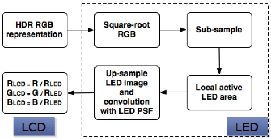
Figure 2-17: Rendering process for a LED-based HDR display ...48

Figure 2-18: Luminance square root method for HDR image splitting ...50

Figure 2-19: Gamut waste (blue region) of luminance square-root method ...55

Figure 2-20: Inaccessible colors (blue region) of luminance square-root method ...55

Figure 2-21: HDR display gamut in normalized XYZ coordinates ...57

Figure 3-1: Print-based HDR display system ...58

Figure 3-3: Calculated matte image ...64

Figure 3-4: Crop the images ...65

Figure 3-5: Finding correlation blobs ...66

Figure 3-6: Matlab GUI for registration ...67

Figure 3-7: Matlab GUI for demo ...68

Figure 3-8: Projector linearization measurement ...69

Figure 3-9: Spectral radiance under uniform projection ...70

Figure 3-10: Normalized spectral radiance under uniform projection ...71

Figure 3-11: Chromaticity shift at different digital counts ...72

Figure 3-12: Projector LUT ...72

Figure 3-13: Form factor compensation image ...74

Figure 3-14: Measurement spots to verify uniformity correction ...75

Figure 3-15: (a) HP Photosmart Pro B9100 printer, (b) Gretag Macbeth Eye-One Isis ....77

Figure 3-16: (a) Characterization chart and (b) its reference file ...78

Figure 3-17: Screenshot of Photoshop setup to print characterization target ...79

Figure 3-18: Screenshot of the Profilemaker when making profile ...82

Figure 3-19: Workflow for evaluating printer ICC profile prediction ...83

Figure 3-20: Convert to profile with absolute colorimetric intent ...84

Figure 3-21: Measurement data file ...84

Figure 3-22: Color difference histogram ...85

Figure 3-23: Color difference vector plot ...86

Figure 3-24: Printer gamut achieved on HP premium paper ...87

Figure 3-25: Combined projected and print image to check registration accuracy ...89

Figure 3-26: Color gamut of printer on HP satin matte advanced photo paper (mesh) and HP canvas (solid): (a) plotted in Lab space (b) plotted in xyY space ...91

Figure 3-27: Actual photo of dual-projector-based HDR display ...95

Figure 3-28: Projector-based HDR display ...95

Figure 3-29: HDR display built in Munsell lab ...96

Figure 3-30: Projector’s neutral behavior check (circles represent measured values) ...98

Figure 3-32: (a) The DLP LUT under standard mode, and (b) the DLP LUT under

dynamic mode ...101

Figure 3-33: Registration targets ...103

Figure 3-34: Alignment setup for HDR display ...103

Figure 3-35: Registration flowchart ...105

Figure 3-36: Flowchart of building HDR display colorimetric model ...107

Figure 3-37: HDR display characterization by using LMT ...109

Figure 3-38: Output luminance as a function of back and front panels ...110

Figure 3-39: (a) LCD red channel LUT. (b) LCD green channel LUT. (c) LCD blue channel LUT. (d) Projector LUT ...111

Figure 3-40: Scatter plot of CIEDE94 against a*b* for 216 factorial data ...112

Figure 3-41: Color difference histogram (Projector with filter) ...113

Figure 3-42: Color difference histogram (Projector without filter) ...114

Figure 3-43: A vertical line formed by single pixel ...115

Figure 3-44: Expanded vertical line formed by single pixel ...116

Figure 3-45: Comparison of MCSL HDR display primary and sRGB primary ...117

Figure 3-46: Gamut of the MCSL HDR display ...118

Figure 3-47: R, G and B primary spectra ...119

Figure 3-48: Spectra of projector white ...119

Figure 3-49: Transmittance spectra of LCD color filter ...120

Figure 4-1: iCAM06-based image splitting flowchart ...123

Figure 4-2: iCAM06-based image splitting for print-based HDR display ...127

Figure 4-3: iCAM06-based image splitting for projector-based HDR display ...128

Figure 4-4: (a) Square-root LCD image, (b) iCAM06-based LCD image, (c) Square-root DLP projected image and (d) iCAM06-based DLP projected image ...136

Figure 4-5: (a) LCD image and (b) projector image for average surround ...138

Figure 4-6: (a) LCD image and (b) projector image for dim surround ...138

Figure 4-7: (a) LCD image and (b) projector image for dark surround ...138

Figure 4-8: Image colorfulness differences between (a) average and dim surround, (b) dim and dark surround (c) average and dark surround ...141

Figure 5-2: Single rating experiment ...145

Figure 5-3: Pair comparison experiment ...146

Figure 5-4: Average quality ratings given to each image processed by two methods ...148

Figure 5-5: Per image differences between the average ratings for the two algorithms ..148

Figure 5-6: Regression fits to mean image ratings as a function of (a) image dynamic range; (b) average image luminance factor; and (c) image colorfulness ...151

Figure 5-7: Mean score of images for different categories ...152

Figure 5-8: Paired comparison results on all five attributes ...154

Figure 5-9: Paired comparison results for different image categories ...155

List of Tables:

Table 2-1: Color appearance phenomenon [Fairchild 2005] ...16

Table 2-2: Comparison of film and digital camera ...22

Table 2-3: Variants of the LogLuv format ...30

Table 2-4: HDR display elements ...44

Table 3-1: Projector setting for print-based HDR display system ...61

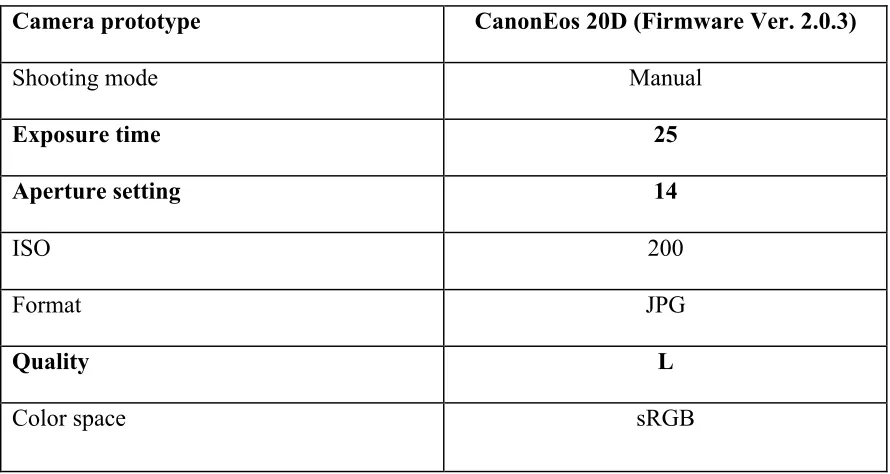
Table 3-2: Camera setting for geometric registration ...64

Table 3-3: Luminance measurement on spots 1 and 2 before and after correction. ...75

Table 3-4: Devices involved in characterization ...76

Table 3-5: Printer temporal stability CIEDE2000 error ...81

Table 3-6: Profile accuracy evaluation ...85

Table 3-7: Theoretical registration accuracy for print-based HDR display ...88

Table 3-8: Performance of print-based HDR display ...90

Table 3-9: LCD front panel setting ...97

Table 3-10: Projector setting for HDR display system ...99

Table 3-11: Measurements of the center of the white screen under different modes ...99

Table 3-12: Camera setting for HDR display geometric registration ...104

Table 3-13: Color differences before and after optimization (Projector with filter) ...113

Table 3-14: Color differences before and after optimization (Projector without filter) ..114

Table 4-1: Values of gamma in surround adjustment functions ...133

Table 4-2: Image colorfulness under different surround settings ...139

Table 5-1: Parameters of the regression fits ...152

1 Introduction

High dynamic range imaging (HDRI) is a set of techniques that allow a greater dynamic

range of luminance to be captured, stored and displayed compared to current standard

digital imaging techniques or photographic methods. This new HDRI technique allows a

more accurate representation of the real world scenes, ranging from faint starlight to

direct sunlight.

The goal of this thesis project is to develop an image splitting algorithm for building high

dynamic range (HDR) displays. Unlike conventional display system, HDR display uses

two optically coupled imagers to extend the dynamic range. This dual image plane design

requires that a given HDR input image be split into two complementary standard

dynamic range (SDR) components that drive the coupled systems; therefore, there exists

an HDR image splitting issue. To better describe, this chapter briefly overviews the

background and development of HDRI, and how it is incorporated into this study, which

is on building HDR displays.

1.1

Background

Dynamic range in this research is defined as the ratio between the brightest and darkest

luminance in a scene. Real-world scenes cover luminance levels as shown in Figure 1-1

from below 0.001 candelas per meter-square (cd/m2) to over 10,000 cd/m2 [Johnson

2005]. Therefore, the overall dynamic range we perceive is as vast as 10,000,000:1. In a

Figure 1-1: Approximate luminance levels in the real world scenes [Johnson 2005;

Ferwerda 1996]

Luckily, despite the fact that the real world scene could have a dynamic range of nearly

14 orders, over 9 orders of luminance magnitude [Kuang 2006] can be adapted by the

human visual system. The way that the human visual system works is through the

photoreceptors (namely rods and cones) on the retina, which then send the signal through

optic nerves to the brain, and finally an image is formed. As is suggested from Figure

1-1, the rods are extremely sensitive to light and provide achromatic vision at scotopic

levels of illumination, where color information is hardly perceived since the cones are

inactive. When the luminance level rises, the cones begin to function between 0.001 and

3 cd/m2 [CIE 1978]. This range is named the mesopic range where both photoreceptors

function. With a further increase in the luminance level, the rods saturation begins, and

the range where only the cones work is named photopic vision. Through slow adaptation

(mechanisms due to photopigment bleaching) in minutes, the human visual system is able

to the pupil and neural reactions), the eye’s static range is smaller, around 10,000:1, but it

still exceeds the capabilities of conventional imaging and display techniques.

Current digital cameras are significantly limited in capturing the full spectra content and

dynamic range of the outside world. Their captured dynamic range is between 100 or

1000 to 1 around a level set by aperture and shutter speed. There are also storing

problems, since even given a means of generating or acquiring dynamic range data, the

conventional file formats are incapable of accurately storing it. The same problems exist

in display technology. Conventional display systems are similar in that their output

dynamic ranges are on the order of 100 to 1 with maximum luminance output levels

around 80 cd/m2 and 250 cd/m2 for typical CRT displays and LCD displays [Xiao 2005]

respectively. Reflective media such as print paper has an even narrower dynamic range,

in most cases much less than 100:1 [Reinhard 2006].

1.2

HDR Imaging Development

Due to the always existing discrepancy between the real world dynamic range and the

limited dynamic range reproducibility of various media (paint, film, print and digital

images), research relating to HDRI actually started thousands of years ago.

1.2.1

Old Solutions

A long time ago, in the painting field, master painters made great effort to record the

using their special painting skills. The Magpie (Figure 1-2), an oil painting by Claude

Monet in1869, is an example that illustrates his marvelous painting technique to achieve

a high contrast in a snowy landscape.

For example, Monet painted the snow in high key while reinforcing the contrast with the

dark tree bark. At the same time, he made subtle variations in the shadow colors, from the

yellow tint of the sun to the cooler, bluish portion of the sky, and since our eyes are more

sensitive to local contrast, increasing these local details increase the overall perceived

contrast of the scene.

Figure 1-2: The Magpie by Claude Monet, 1869.

When film-based photography was invented, it used the action of light to cause changes

in a film of silver halide crystals in which development converts exposed silver halide to

metallic silver. However, capturing the enormous dynamic range of luminance on a

design film stocks and print development systems that gave a desired S-shaped tone

curve with slightly enhanced contrast in the middle range and gradually compressed

highlights and shadows [Hunt 2004]. To further solve the problems of silver halide

negatives having a greater dynamic range than the print media, “dodge and burn”

technique [Adams 1995] is introduced to manipulate the exposure of a selected area on a

photographic print. Dodging decreases the exposure for areas when the photographer

wishes it to be lighter, while burning is the reverse process that increases the exposure to

areas that should be darker in the print. Since this method effectively adjusts the local

contrast, it therefore leads to an improvement of the overall perceptual contrast in a

photograph. The only issue is that the same procedure has to be done for each print,

which can be quite time consuming.

1.2.2

Digital HDR imaging

With the advancement of digital photography and computer graphics, the imaging

industry will inevitably transit to HDR imaging with devices that provide a far greater

range. This completely overthrows traditional imaging techniques and requires a new

workflow, which can be seen in Figure 1-3. The HDR capture and storage side has the

same path, but for the display side, there are two paths: one leading to a SDR display

requiring tone-mapping techniques in order to compensate dynamic range differences.

The other path uses HDR display allowing the direct display of HDR content. Note that

for the convenience of the readers, a tone-mapped version of the HDR scene is used in

Figure 1-3: HDR digital imaging pipeline.

For capturing HDR scenes, methods for acquiring HDR images from multiple SDR

images have been established in recent years. This technique was first investigated by

Mann and Picard in 1995 [Mann 1995], and Debevec and Malik brought it into computer

graphics in 1997 [Debevec 1997]. Other research followed and include the work done by

Mitsunaga and Nayar [Mitsunaga 1999], Robertson [Robertson 1998], etc. that focus on

HDR still images capture. As for capturing HDR video, Kang proposed a method based

on a similar technique [Kang 2003]. The above technique involves merging several

images taking at different exposure times into one HDR image. Besides this

multi-exposure technique, recent advances in image sensor technology have the potential to

directly capture higher dynamic range using only one shot (More information is provided

in Chapter 2.).

For HDR storage, it employ a color space corresponding to particular output devices

different from current output referred standards. It is scene referred, meaning that the

Therefore it requires efficient representation that covers the full range of color values,

usually a luminance step size below 1% and good color resolution, as close to perfect as

the human vision’s discerning capability [Ward 2006]. Chapter 2 provides more detailed

description of recent work on HDR encodings, including Radiance RGBE encoding,

JPEG-HDR encoding, OpenEXR and etc.

For displaying HDR contents, there are two paths: one displaying on a SDR display

requiring pre-processing the HDR image by using HDR rendering algorithms or known

as tone-mapping operators (TMOs) to compensate for the dynamic range difference, and

at the same time, achieve a faithful visual representation of original scene. The other path

is displaying HDR contents on an HDR display directly where related research has also

been very fruitful in the last few years. In 2004, Ward and Seetzen et al. [Seetzen 2004]

constructed two different prototypes that vastly exceed the dynamic range of

conventional softcopy displays. In 2008, Bimber extended this idea to reflective media

and created a hardcopy HDR display system [Bimber 2008]. Currently, Dolby Inc. is

dedicated to bringing the softcopy HDR display technology to other manufacturers, thus

someday making HDR displays available to every household.

1.2.3

HDR image splitting issue

As stated in the above, the principle of building HDR display systems is double light

modulation that reproduce high dynamic range images by using two SDR imagers that

are optically coupled. As is shown in Figure 1-4, one imager (such as a projector or LED

transmissive LCD or reflective print), allowing HDR values to be reproduced by the

combination of the two. This dual image plane design requires that a given HDR input

image be split into two complementary SDR components that drive the coupled systems.

Therefore, there exists an HDR splitting issue for driving HDR displays.

Figure 1-4: Image splitting issue in building HDR display.

Work is just beginning on HDR image splitting algorithms and some of this work is

proprietary, but several algorithms have been published. The most widely used HDR

image splitting method is the luminance square root algorithm [Trentacoste 2007]. It first

converts an input HDR image to XYZ tristimulus values, then takes the square root of the

Y channel and sends this achromatic signal to one image plane, while also sending a

color signal created by composing

!

Ywith its corresponding X and Z channels to the

other image plane. Under ideal conditions this approach will reproduce the original

luminance range of the HDR input, but good color appearance reproduction is not

guaranteed or usually not even considered. Recently, Luka and Ferwerda [Luka 2009]

introduced a variation on the square root algorithm that accommodates HDR displays

improved the saturation of dark colors.

Guarnieri et al. [Guarnieri 2008] developed an HDR display for radiological applications

by layering two high quality grayscale medical LCD displays. Due to the critical nature

of the application, they were concerned with the accuracy of the displayed image and

effects of the image splitting algorithm on the visibility of image features. They

developed an optimization-based HDR image splitting algorithm that simultaneously

considered luminance reconstruction errors and spatial parallax errors caused by the

thickness of the layered LCD panels. They approached HDR image splitting as an

optimization problem and have produced an algorithm that typically achieves perfect

luminance reconstruction and minimal parallax errors. When a perfect reconstruction is

not possible, errors are minimized through the application of a visible difference metric.

While this algorithm is based on sound mathematical and perceptual principles, it is

designed to handle grayscale radiological images shown on a dual layer LCD display and

is not directly applicable to the general class of color HDR images or other HDR display

technologies.

1.3 Research goal

The goal of this thesis is to develop a new HDR image splitting algorithm that will create

displayed HDR images with improved image quality and also take image appearance

phenomenon into account by taking a more principled approach to the HDR image

splitting algorithm. To achieve this goal, this thesis work includes building both hardcopy

algorithm, and testing the resulting performance by psychophysical methods.

1.3.1 Building HDR displays

For the softcopy HDR display, the previous dual projectors-based HDR display system in

the Munsell Color Science Laboratory (MCSL) built by graduate student Stefan Luka

[Luka 2009] was modified to a single projector-based HDR display. For the hardcopy

HDR display, following the previous work done by Bimber [Bimber 2008], a print-based

HDR display was built. More details on display setups, building the displays, and their

colorimetric performance are described in Chapter 3.

1.3.2 Developing iCAM06-based image splitting algorithm

In color appearance phenomenon, color appearance models or image appearance models

are involved. The image appearance model iCAM06 was incorporated proving to be an

efficient model for both preference and accuracy in the rendering of SDR displays split

into a single HDR image. The ultimate goal is to make the recombined image approach

its actual appearance in a given viewing condition as close as possible. More details on

iCAM06 algorithm and its implementation into HDR and image splitting algorithm is

found in Chapter 4.

1.3.3 Testing the performance of HDR image splitting methods

Since observers are the final output of HDR display systems, the best way to verify an

algorithm’s performance is through psychophysical studies. In this project, both single

performance of the iCAM06-based HDR image splitting method to the widely used

square root luminance method. For the convenience of conducting the experiments, only

a softcopy (projector-based) HDR display is employed to collect the observers’ response.

1.4 Document structure

After the present chapter, which serves as an introduction to this study, Chapter 2 will

give an overview of previous work relating to this research interest and including an

introduction to color science, color and image appearance, HDR image capture, storage,

HDR displays, the human visual system, tone-mapping operators, and HDR image

splitting algorithms. Chapter 3 describes the detailed process of building both a

print-based and a projector-print-based HDR display. The new iCAM06-print-based image splitting

algorithm is then described in detail in Chapter 4. Next, Chapter 5 illustrates experiment

framework to compare the splitting algorithms’ performance between the new method

and the widely used square root method. Finally, conclusions and some possible future

directions are available in Chapter 6.

2 Literature Review

This literature review describes the previous work that relates to this thesis project. It

covers the basic theory of color science, color management, and state-of-art descriptions

of the HDR digital imaging pipeline and HDR image splitting algorithms.

2.1 Colorimetry, color appearance and image appearance

Colorimetry is the science and technology used to quantify and describe physically

human color perception [Ohno 2009]. According to a classic color science book by

Wyszecki and Stiles [Wyszecki 1982], colorimetry falls into two categories: (1) basic

colorimetry and (2) advanced colorimetry.

The basic colorimetry describes the nature of color perception, how to quantify this

perception by measurement device and judgment of whether two visual stimuli match.

Many of the basic colorimetry problems of color differences, chromatic adaptation, and

color appearance are well defined and solved. Advanced colorimetry finally leads to the

color appearance of color stimuli presented to the observer in complicated surroundings.

Next, image appearance models that include spatial and temporal vision properties for

image difference evaluation or HDR image rendering are also studied.

2.1.1 Basic colorimetry

In color perception, the three necessary elements are objects, light sources, and the

For the study of light sources, the CIE (International Commission on Illumination)

published a series of well-known standard illuminants such as CIE standard illuminant A,

D65 and D50. More detailed information can be found on the CIE website [CIE 2003]:

These standard illuminants provide a basis for comparing colors recorded under different

lighting.

For the study of objects, light interacts with the object material by reflection,

transmission and absorption with terms of reflectance (ratio of reflected energy to the

incident energy), transmittance (ratio of transmitted energy to the incident energy) and

absorbance (ratio of absorbed energy to the incident energy). Accurate measurement of

theses parameters are needed to quantify color perception. These parameters are not only

a function of wavelength, but also a function of the illumination and viewing geometry.

The CIE recommends measurement geometry (bidirectional 45/0 and hemispherical d/0),

explained in the Principles of Color Techonology [Berns 2000], but to get a complete

measurement of these parameters, bidirectional reflectance distribution functions

(BRDFs) need to be obtained requiring a thorough point-wise measurement of object

reflectance taking both light source input angles and output angles into account. More

information on BRDF definitions and BRDF models (such as Ward model [Ward 1992]

and Cook-Torrance model [Torrance 1967]) can be found in the Digital Modeling of

Material Appearance [Dorsey 2008].

facilitate human perception. Color perception is first mediated by cones with sensitivity

in the long (L(λ)), middle (M(λ)) and short wavelength (S(λ)) region of the spectra. To

further develop the relation between cones’ spectral response function and calculation of

color perception, color matching experiments were first performed in 1931 to drive the

color matching functions (CMFs) of a small number of color normal observers. They

were later transformed to XYZ primaries to eliminate the negative values and force one

of the functions equal to the CIE 1924 photonic luminous efficiency function (V(λ)).

Later, they were adopted by the CIE as the CIE 1931 standard observer and are widely

used to calculate color perception in the industry. Several years later, the CIE 1964

standard observer was proposed to extend the viewing angle from 2° to 10°. The research

interests in defining color matching functions is ongoing. In 2006, the CIE 2006 model is

defined as a convenient framework for calculating CMFs for any field size between 1°

and 10° and age between 20 and 80 years [Fairchild 2007].

By knowing the relevant parameters of objects, light sources and the human visual

system, color could be digitally defined by XYZ tristimulus values. But there are several

limits of the XYZ color space (uniformity issue and etc.) leading to the development of

opponent color spaces such as CIELAB, CIELUV, etc. Since it is not intended to provide

complete details about colorimetry here, more details and information are available in the

2.1.2 Color appearance model

In everyday life, color is not viewed alone as the surrounding environment also has a big

effect on color perception and as the human visual system adapts to this environment.

Furthermore, there are various color appearance phenomena (listed in Table 2-1) that fail

to be accounted for in basic colorimetry.

Note that for the study of these effects listed in Table 2-1, viewing flare is usually not

considered. For example, the Bartleson-Breneman that the darker the surround, the less

perceived contrast is opposite to our daily life experience since when we view image in a

dark surround, we will feel that the contrast is increasing comparing to the surround with

the a light turned on. This is because of flare in the viewing condition which is very

difficult to avoid without careful control.

The various color appearance models, such as the Nayatani et al. model [Nayatani 1990],

the Hunt model [Hunt 1994], the RLAB model [Fairchild 1996]; CIECAM97 model [CIE

1998] and CIECAM02 [CIE 2004] were developed to incorporate these phenomenon on

color perception.

Though the detailed equations of each model differ a lot from each other, these models

proceed with the following three main steps: (1) Chromatic adaptation: the estimation of

the color perception under different light sources, (2) Nonlinear response compression:

computation of perceptual appearance correlate that usually include lightness, brightness,

hue, chroma, colorfulness and saturation.

Table 2-1: Color appearance phenomenon [Fairchild 2005].

Color appearance phenomenon

Example Explanation

Simultaneous contrast

Shift in color appearance when the background color is changed.

Crispening Increased in perceived color difference magnitude due to the similarity of

background and stimuli.

Spreading

Apparent mixture of a color stimulus with its surround.

Bezold-Brucke hue shift

Perceived hue changes with luminance. Plot shows the wavelength shift required to maintain a constant hue.

Abney effect

Perceived hue changes with colorimetric purity.

Plot shows constant hue in the CIE 1931 chromaticity diagram.

H-K effect

Brightness depends on luminance and chromaticity. Plot shows contours of constant brightness-to-luminance ratio.

Hunt effect

Colorfulness increases with luminance. Plot shows corresponding chromaticities across changes in luminance.

Stevens effect

Perceived lightness contrast increases with increasing adapting luminance.

Helson-Judd effect Nonselective samples do not appear neutral under strongly chromatic

illumination.

Bartleson-Breneman

These models are capable of predicting the appearance of spatially simple color stimuli

under a wide variety viewing conditions. However, such models do not directly

incorporate any of the spatial or temporal properties of human vision and the perception

of complex stimuli such as images. Therefore, there is research interest in developing

image appearance models for when a stimulus is observed in practice in a much more

complicated viewing environment than a uniform field under a given luminance.

2.1.3 Image appearance model

Image appearance models account for more complex changes in visual response by

extending color appearance models to include spatial vision, temporal vision and image

quality properties [Fairchild 2005]. Therefore, given an input images and viewing

conditions, an image appearance model can provide perceptual attributes of each pixel by

taking human visual system into account.

The first stage of the development of image appearance models is to incorporate

convolution kernels to approximate the contrast sensitivity function (CSF) of the human

visual system [Zhang 1996]. Therefore the information that is less sensitive to human

perception is removed when evaluating per-pixel image differences. Later, other spatial

models are developed: CVDM [Elaine 1998], Sarnoff Model [Lubin 1997], and MOM

[Pattanaik 1998]. However, these models are either not powerful enough for general

image appearance prediction or computational expensive: therefore, iCAM [Johnson

2003] was developed to combine the knowledge about color appearance, spatial vision

get an adapting image for calculating per-pixel based chromatic adaptation, then use an

exponential function to modulate image (a kind of gamma factor) at a per-pixel basis.

The iCAM image appearance model accounts for local image information and therefore

shows great potential in image appearance prediction, image difference metrics and HDR

image rendering.

Based on the iCAM framework, iCAM06 was developed especially for HDR image

rendering applications with some improvements to achieve more pleasant and accurate

HDR rendering [Kuang 2007]:

(1) Bilateral filter technique: to separate the image into a base-layer and a detail-layer by

utilizing its edge-preserving feature. The base layer is obtained using a non-linear

bilateral filter where each pixel is weighted by the product of a Gaussian filter in the

spatial domain and another Gaussian filter in the intensity domain (shown in Eqs. (2-1)

and (2-2)).

(2-1)

(2-2)

Where Is is the intensity value for pixel s. k(s) is a normalization term, f() is a Gaussian

function in the spatial domain with the space kernel scale σs and g() is another Gaussian

function in the intensity domain with its range kernel scale σr. The space kernel scale σs

J_s = 1

k(s)p"#

$

I_P

k(s)= f(p!s)g(I_P !I_S) p"#

affects the size of the considered neighborhood and the range kernel scale σr controls the

amplitude of the edge. σs is similar to the common Gaussian blur application. The bigger

the σs, the more neighborhood is included in the result and higher accuracy is achieved at

the sacrifice of lower computation speed. The bigger the σr, the faster the computational

speed but less edge information will be preserved. An example is provided in Figure 2-1

[Paris 2007], to preserve more image details, range scale σr that relates how accurate the

edge information can be preserved is a more critical setting.

Figure 2-1: Illustration of bilateral filter theory.

To achieve both a satisfying result and reasonable computational speed, σs is set to

empirical value of 2% of the image size and σr is set to a constant value of 0.35 [Kuang

2007]. With bilateral filtering technique, edge and detail information of the original input

image are better preserved.

(2) Replace the simple non-linear local gamma correction in iCAM with the

photoreceptor response functions from previous color appearance research. It uses a

linear von Kries normalization of the spectral sharpened RGB image signals by the RGB

adaptation white image signals at each pixel location.

(3) Extend to a larger range of luminance by incorporating scotopic and photopic vision.

The rods’ and cones’ response functions are calculated separately and the final tone

compression response is a sum of the two.

(4) Simulate the colorfulness changes predicted by Hunt effect by incorporating a

luminance dependent local colorfulness enhancement module.

(5) Simulate the contrast change suggested by the Stevens effect by incorporating a

luminance dependent local contrast enhancement module.

(6) Simulate Bartleson-Breneman surround effect by incorporating a luminance

dependent correction module.

Steps (4) to (6) are done in IPT color space. First, the tone-compressed RGB signals are

converted back to CIE XYZ image and combined with the detail image layer. Next, the

combined CIE XYZ image is converted into the IPT uniform opponent color space. P and

T adjustments are used to predict Hunt effect, and a power function is applied to the I

channel in IPT space to account for Bartleson-Breneman surround effect [Kuang 2007].

2.2 HDR image capture

Two media (film and an electronic image sensor) are usually involved in photography.

Though the basic techniques of the two are quite different, they share many common

features. For better understanding, comparisons of the two are listed in Table 2-2

[McCann 2010].

The lens and camera body are the same for film and the digital camera processes. The

sensor processing is different, one is mainly chemical process and the other one is digital

image processing, but the basic imaging principles of the two are the same. Therefore, in

order to enhance the dynamic range of these two media, they can share a similar idea of

using the multi-exposure technique which will be described later in this Chapter. The

difference is that they will be conducted differently based on their individual medium

characteristics. Detailed descriptions of extending the dynamic range of film and digital

cameras will be described in separated section.

Table 2-2: Comparison of film and digital camera.

Components Film Digital

Lens Aperture, F number,

coating, resolution Same

Camera Volume, surface Same

Sensor Resolution, spectral &

dynamic range

Same

Sensor processing Developer, stop bath,

hypo, hypo clearing, tone, wash (B&W).

A/D, noise reduction, de-mosaic, sharpening,

color enhancement.

Storage Dry negative Digital file

2.2.1 Capture by film scanning

Film camera records a nearly 10,000:1 dynamic range by film emulsions [Reinhard

2006]. To record the full log range of the negative film in an HDR format, a film scanner

with know response curve needs to be used. Once a scanner’s file format is obtained, it is

then “developed” this file at several different exposures and merged into one image in

HDR format.

2.2.2 Capture by digital camera

To better illustrate the HDR image capture issues for a digital camera, the image

processing pipeline of a typical digital camera is illustrated in Figure 2-2 [Liu 2002]. The

light passes through the lens and is projected on the color filter array (CFA) then

converted into electrical signal by the CCD. Next, the signal is amplified by the

automatic gain control (AGC) and converted into a digital signal by an ADC (analog to

digital converter). Finally, the image is processed (demosiacing, auto white balance, color

correction, gamma correction, etc.), enhanced, compressed (such as JPEG), then stored.

Since the lens is merely a passive element that refocuses the incoming light, the

limitation of dynamic range is caused mainly by sensor structure design. It is quite

difficult to improve the sensor’s ability to capture the dynamic range of a real scene,

since, for sensor manufactures, there are tradeoffs between dynamic range and contrast,

pixel size and noise level, and etc., and for most current cameras, the captured range is

the real world dynamic range. Figure 2-3 provides a concrete example that illustrates

some of these tradeoffs.

Figure 2-2: Digital camera image processing diagram [Liu 2002].

In this example, a tree with yellowish leaves in direct sunlight produces high luminance

while the rock near the lake is quite dark. If the camera’s exposure is set to capture detail

in the rock, the bright tree is blown out and the its detail lost. If we set the camera’s

exposure to capture detail in the tree, the rock will be totally dark and no detail preserved.

Therefore we need several separate shots from the traditional camera to make each pixel

from the bright tree to the dark rock properly exposed.

2.2.2.1 Multi exposure capture

In order to take HDR image using a traditional camera, the most accessible way is to take

more than one photograph of the same scenes covering different exposure times from

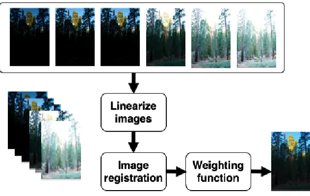
under-exposed to over-exposed images. The flowchart is illustrated in Figure 2-4. There

are three main steps for merging these images taken at various exposure times into one

HDR image.

First is linearization, which involves measuring the tone curves of the camera. They can

be measured by taking images of step-chart or OECF chart under uniform illumination

(lightbooth or 45° projecting light on both sides) or by sampling the camera response

function at each pixel under the scene captured at different exposures [Debevec 1997],

Figure 2-4: Flowchart of the multi-exposure technique.

Next is image registration which is a crucial part of final image quality since HDR

capture involves taking several images and it is rare that the camera can be held stable

during capture. There are several techniques developed in the past years that account for

camera and object movement in a scene by estimation motion variance [Kang 2003].

MTB (mean threshold bitmap) is proposed by Greg Ward that finds the least shift errors

of all pixels to achieve best image alignment [Ward 2003].

Finally, the final HDR image is computed as a weighted sum of these images. Mann used

the derivative of the system response curve as the weighting function [Mann 1995];

Robertson used a Gaussian-like function as the weighting function [Robertson 2000]. The

latter work assumes that the mid-range pixels are more reliable. The weighting function

reflects the certainty with which the value of an individual pixel in any of the input

2.2.2.2 Direct capture

In recent years, sensors which can capture a full dynamic range of a scene in a single shot

have been developed and some are commercially available: the Autobrite cameras from

SMaL Camera Technologies, the SpheroCam HDR panoramic camera (shown in Figure

2-8) from Spheron VR and the Ladybug spherical camera from Point Grey Research. One

example is placing an optical mask with spatially varying transmittance adjacent to a

conventional image detector array thereby giving adjacent pixels on the detector different

exposures of the scene [Nayar 2000], thus makes the capture of an outstanding HDR

image in a single pass possible. The final HDR image is reconstructed by aggregation and

interpolation. This technology has the advantage of producing an HDR image in real time

and is applicable to moving scenes. The shortcoming is that most current equipment are

very expensive and thus limited to commercial use.

But with more and more attention on HDR capture, an HDR camera will be available to

the consumer market in the near future. Recently, iPhone 4 developed a new HDR feature

that takes 3 frames at different exposure times and merges then into one HDR image.

After tone-mapping, it can be directly viewed on the retina display of an iPhone 4. The

whole process takes about 5-10 seconds, and for the scene with higher dynamic range, the

final tone-mapped image quality (better color reproduction, more detail, more contrast,

etc.) is quite satisfying than that of the single-exposure image, therefore future HDR

capture applications should not be limited to the DSLR camera market since it already

Figure 2-5: SpheroCam HDR panoramic camera picture [Sphero 2010].

2.3 HDR image formats

Traditional RGB image formats are tailored for traditional display devices, therefore the

color gamut is constrained by red, green and blue monitor phosphors and the luminance

encoding is often limited to 2 orders of magnitude. Formats such as JPEG and GIF

provide 8 bits per color channel, RAW and PNG offer up to 16 bits per color channel, but

most of them represent exactly the same color gamut. So they are still not capable of

encoding HDR image information.

There is a need for a common format that could be understood by both HDR capture and

HDR display to better encode color gamut and luminance of the real world scenes that

facilitates the HDR digital imaging pipeline. Requirements [Ward 2006] for encoding

HDR image are listed below followed by a review of a few of the main HDR image

(1) Luminance encoding: the quantization error should be below 1% with more than

12 orders of magnitude.

(2) Faithfully represent the full visible color gamut.

(3) Better correlate with perceptually uniform luminance and good color resolution to

be able to encode any image with fidelity as close to the human vision’s

discerning ability.

2.3.1 Higher Precision Encodings

The simplest way for HDR image storage is to extend the RGB components to 32-bit

floats point directly like the 96-bit IEEE TIFF. Obviously it has high enough precision,

but the resulting huge size multiplier (up to 36MB as an uncompressed) will cause a lot

of trouble in storage and compression, thus limits its real application.

2.3.2 Pixar Log Encoding (TIFF)

This format was proposed by Pixar for use in film recording since film has a greater

dynamic range than a standard 24-bit/pixel image and a logarithmic encoding for RGB

values. By utilizing this representation, this format was able to encode a dynamic range

of about 3.8 orders of magnitude in 0.4% steps [Holzer 2008] meeting the requirement of

the 1% luminance visible JND threshold [Ward 2006]. However, this format has limited

application since it was used internally at Pixar and is not well-known to the computer

2.3.3 Radiance RGBE/XYZE Encoding

The Radiance RGBE format is probably the most widespread in the HDR imaging

community. It has one byte for the red, one byte for the green, one byte for the blue and

one for a common exponent used as a scaling factor on the three channels as is shown in

Figure 2-6. Thus it has 32 bits/pixel covering a luminance range of over 76 orders of

magnitude at the expense of absolute accuracy, which is still about of about 1% and is

just sufficient for surpassing human perception [Holzer 2008]. Besides, since it only

supports positive RGB values, it cannot represent all colors of the visible gamut [Ward

1998].

Figure 2-6: Bit distribution of Radiance RGBE/XYZE [Holzer 2008].

To fix this problem, XYZE was developed which uses the “imaginary” primaries of the

CIE XYZ color space instead of the “real” primaries thus extending the range of color to

the entire visible gamut [Ward 2006].

2.3.4 SGI LogLuv (TIFF)

SGI LogLuv was proposed by Ward at SGI to create a more efficient or perceptual-based

encoding than Radiance RGBE. This encoding is based on visual perception and

of JPEG YCC encoding, they both separate the luminance logarithmically and

chrominance values (CIE u’v’) linearly in separate channels, as shown in Table 2-3

below. The first variant (LogLuv24) is able to cover a dynamic range of 4.8 orders of

magnitude in uniform 1.1% steps but causes visible artifacts due to the limited luminance

range [Roimela 2006]. The second variant (LogLuv32) consists of 15-bit encoding of

luminance covering a range of 38 orders of magnitude in 0.3% steps [Ward 2006]. Both

variants are a part of Leffler’s TIFF library [Ward 2006].

Table 2-3: Variants of the LogLuv format.

Variants Luminance Chrominance Diagram

LogLuv24 10 bits 14 bits

LogLuv32 16 bits 16 bits

2.3.5 ILM OpenEXR (EXR)

Starting in 1999, Industrial Light and Magic (ILM) developed OpenEXR, a HDR image

file format for use in digital visual effects production. In early 2003, ILM published open

source code for reading and writing the OpenEXR image format.

It supports 32-bit floating point precision per component, but its primary form is a 16-bit

floating point per RGB-primary encoding (half-format) divided into 1 sign bit, 5

exponent and 10 mantissa bits [Holzer 2008]. This half format supports de-normalized

numbers, positive and negative infinities and NaNs. It is able to covert the entire visible

Since it is identical to the half data type in NVIDIA’s Cg graphics language, there is a

convenient transplantation from OpenEXR image directly to the current NVIDIA GPUs.

All these unique features of OpenEXR make it a good fit for high-quality image

processing and storage applications [Kainz 2009].

2.3.6 Microsoft/HP scRGB encoding

A new set of encodings named scRGB for an HDR image representation has been

proposed by Microsoft and Hewlett-Packard (HP). This grew out of the sRGB

specification widely used for SDR encodings. The scRGB standard is divided into two

parts, one employing 48 bits/pixel in an RGB encoding and the other employing 36

bits/pixel either as RGB or YCC. In the 48 bits/pixel encoding, though it considerably

improves sRGB, it cannot represent the full gamut at higher luminance levels reducing its

precision and limiting its dynamic range to about 3.5 orders of magnitude [Ward 2006].

In the 36 bits/pixel encoding, though it uses 25% fewer bits, its dynamic range is 3.2

orders close to 48-bit version. But it has similar disadvantages at the top end of the gamut

with less dynamic range limiting its commercial use and requires further improvement

[Holzer 2008].

2.4 Human visual system and HDR tone mapping

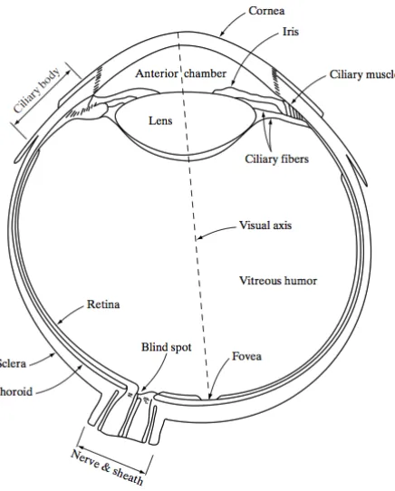
The human eye acts like a camera. The cornea is a transparent structure in the front of the

is finally focused onto a light sensitive membrane call the retina that is illustrated in

Figure 2-7.

Figure 2-7: Human eye [González 2008].

Through local adaptation, the human visual system can perceive a dynamic range about

10,000:1 [McHugh 2011] exceeding the capabilities of conventional display techniques

by several orders of magnitude. Therefore to reduce this dynamic range discrepancy and

display an image with realism, HDR tone mapping techniques are actively being studied.

2.4.1 Tone mapping problems

In order to fit the dynamic range of a HDR scene into a SDR display, the simplest way is

scene are lost. To solve this problem, visual models are used when mapping dynamic

range. The ultimate goal is to reproduce the visual appearance of the original scene on a

SDR display. Current tone mapping operators could be classified as global operators or

local operators.

2.4.2 Tone mapping operators

The HDRI book [Reinhard 2006] gives a good review of a number of tone mapping

operators intended to map HDR images to SDR displays.

2.4.2.1 Global operators

For a global operator, every pixel in the image is mapped the same way by a non-linear

functions based on the luminance and other global variables independent of a pixel’s

position. One global image adjustment tool is the Photoshop Curve Tool which take input

tone scale and selectively stretches or compress them. Similar to the “S-curve” that

applied to film industry, a “S-curve” for this global adjustment can add contrast to the

midtones that are perceptually more important at the expense of shadows and highlights.

This technique has the advantage that it is simple and fast, but with the sacrifice of some

detail information.

Previous work includes the Miller brightness-ratio-preserving operator and the

Tumblin-Rushmeier brightness-preserving operator. Both operators tend to preserve the brightness;

the difference is that Tumblin-Rushmeier operator attempts to preserve the brightness

brightness-ratio-preserving operators that aim to preserve the brightness sensation, there

are also operators that focus on preserving contrast such as the Ward contrast-based scale

factor and the Ferwerda model of visual adaptation. The difference is that Ferwerda et al.

added a scotopic component to the photopic component. Other work done on global

operators include Ward histogram adjustment [Ward 1997], sigmoid transformation

[Braun 1999], etc.

2.4.2.2 Local operators

Unlike global operators which apply the identical mapping function on all pixels, local

operators assume that a viewer does not adapt to the scene as a whole, but to smaller

regions changing each pixel according to its position and different local operators

handling the local adjustment differently. Previous works include Retinex [Land 1977],

Retinex-based adaptive filter [Meylan 2005], Multiscale observer model (MOM)

[Pattanaik 1998], Bilateral filtering technique [Durand 2002], iCAM [Johnson 2003],

iCAM06 [Kuang 2003] and etc.

Retinex is a word derived from “retina” and “cortex” suggesting that both the eye and the

brain are involved in the processing. Retinex theory explains how the visual system

extracts reliable information from the world despite changes of illumination, which is the

color constancy problem in color science world. The conclusion is that the perceived

color of a unit area could be separated into three parts (long, middle and short) in the

retina depending on not the absolute value of light but the reflectance of objects [Land

theory. Rather than applying a Retinex independently to the R, G, B color channels, they

apply Retinex only to the luminance channel to prevent high contrast losses while, at the

same time, preserve color information [Meylan 2005]. MOM (multiscale observer model)

is based on a multiscale representation of luminance and color processing in the human

visual system [Pattanaik 1998]. It ranks among the more complete color appearance

models. Bilateral filtering is already briefly introduced in Chapter 2 and more details on

its application in iCAM06 HDR rendering could be found in Chapter 4. Different from

the above examples of local operators, the iCAM and iCAM06 models not only aim at

dynamic range reduction, but also serve as image appearance models accounting for

traditional color appearance phenomenon. Other work includes Reinhard’s photographic

tone reproduction operator, Ashikhmin’s operator, etc.

In summary, though the local processing is more complicated than global, local

processing has better performance since local processing can increase both local contrast

and the visibility of some parts of the image. This is quite similar to how human

perception functions and thus allows a better imitation of the human visual system,

therefore leads to better rendered image quality.

2.5 HDR display devices

While the dynamic range of image capture devices can be increased using multiple

capture methods or new imaging sensor technology, high dynamic range display devices

are similar in that their output dynamic ranges are on the order of 100 to 1 with maximum

luminance output levels around 80 cd/m2 and 250 cd/m2 for typical CRT displays and

LCD displays [Xiao 2005]. Let alone the print image, which has even a lower dynamic

range (less than 100:1) due to the limitation of ink properties and optical brightness of the

paper.

In order to provide solutions, research trends lead toward better display devices, which

are capable of displaying images with a dynamic range much more similar to that

encountered in the real world. According to different medium, HDR display devices

could be classified into two major categories: softcopy devices and hard copy devices.

2.5.1 Hardcopy devices

For hardcopy media, there are reflective media and transparent media. But both of them

are inherently LDR and the reasons are illustrated consecutively below:

Reflective media is usually used in printing industry, including traditional ink presses and

digital printing presses, where subtractive color production principles are employed. Inks

with various spectral characteristics absorb particular wavelength of light, which leads to

different color reproduction. The dynamic range of the print image is inherently low,

since it is quite difficult to achieve values in both white and black ends. For white end,

according to colorimetry knowledge, tristimulus values of the white point of reflective

media are determined by both light source and print’s reflectance. Given a light source,

whiten the paper appearance. It usually adopts fluorescent agents, which re-emit light in

the short wavelength region (typically 420-470nm), thus to get more visible light.

However, this could only increase the paper white at a limited extent. As for the black

end, the dyes and pigments have a limited maximum absorption, even if we had best

available absorbing ink, which is generally no better than 99.5% [Reinhard 2006], the

surface of the print itself also reflects light to some extent, thus undermine contrast in the

dark region. Therefore the reflective print media is inherently LDR, with a dynamic range

about 100:1 at best by carefully controlling inks, illumination and background.

Transparent media mostly is designed for projection, such as a 35-mm slide transparency

movie film. Since transparencies rely on a controlled light source and optics, the ambient

environment is under much tighter control, such as in cinema, where transparencies are

viewed in a darkened room with a dark surround. The maximum density, which

determines how dark a transparency can get is only limited by the film chemistry and

printing method. Therefore, though slides and movies are not really HDR, but its

dynamic range (about 1000:1) is bigger than reflective print and has potential to be used

in simple HDR viewers/displays. In order to extend dynamic range of transparent media

and reflective media, HDR still image viewer and reflective HDR display are proposed.

2.5.1.1 HDR still image viewer

The original prototype of HDR still image viewer was created at the Lawrence Berkeley

Laboratory in 1995 to evaluate HDR tone-mapping operators. Later, it is reviewed and

Figure 2-8: Photography of HDR viewer [Ledda 2003].

Figure 2-9: Schematic of HDR viewer [Ledda 2003].

It uses three elements: a bright uniform backlight, a pair of layered transparencies and a

set of LEEP ARV-1 optics. Square root luminance method is used to split a single HDR

image into two transparency layers, which will later be combined in the viewer. A

Gaussian blur function is applied to the back layer to reduce misregistration and parallax

between the two layers. Then by subsequently dividing the back layer into the original,

combination of the two transparency layers is equivalent to adding the densities and the

original HDR view could be achieved by this way. Note that the blurring artifact is less

likely to occur due to alias in human visual system, and this two overlaid transparencies

could achieve a contrast ratio around 10,000:1 [Ledda 2003].

This HDR transparency viewer demonstrates the feasibility of splitting the image into

two layers, which then combined together to produce an HDR view. This idea is of vital

importance to the principles adopted in reflective HDR system and softcopy devices,

which will be explained later.

2.5.1.2 Reflective HDR display

In 2008, Bimber et al. presented a projector-camera system (as is shown in Figure 2-10)

to extend dynamic range of reflective media, such as photographs, radiological paper

prints, ePaper and etc. It also adopts double light modulation and the technique is based

on a secondary modulation of projected light being surface-reflected. And they achieved

physical contrast ratios of 45,000 to 60,000:1 with a peak luminance of more than 2750

cd/m2 [Bimber 2008]. The idea is to figure it out the dynamic range and gamut capability

that could be achieved by the whole system by creating a big LUT, and then square-root

splitting could be applied and the split image could be converted to driving signal of

printer and projector via the LUT. The full printer’s transfer function (printed patch under

projected illuminat