The history of dipper functions

City, University of London Institutional Repository

Citation

:

This is the accepted version of the paper.

This version of the publication may differ from the final published

version.

Permanent repository link:

Link to published version

:

Copyright and reuse:

City Research Online aims to make research

outputs of City, University of London available to a wider audience.

Copyright and Moral Rights remain with the author(s) and/or copyright

holders. URLs from City Research Online may be freely distributed and

linked to.

City Research Online: http://openaccess.city.ac.uk/ publications@city.ac.uk

The History of Dipper Functions

Joshua A. Solomon

ABSTRACT

Dipper-shaped curves often accurately depict the relationship between a baseline or “pedestal” magnitude and a just-noticeable difference in it. This tutorial traces the 45-year history of the dipper function in auditory and visual psychophysics, focusing on when they happen, and why. Popular theories for both positive and negative masking (i.e. the “handle” and “dip,” respectively) are described. Sometimes, but not always, negative masking disappears with an appropriate re-description of stimulus

magnitude.

Introduction, part 1: Gaussian noise

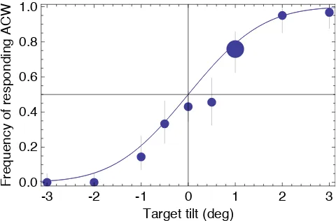
Did you ever have your walls dusted? I did, and the duster (who shall remain nameless) managed to knock all my pictures out of alignment. You can try, but it is impossible to hang a picture perfectly straight. Sometimes the right side seems a little too high, sometimes it is the left side. I would change my mind even without moving the picture. This uncertainty is manifest in psychometric functions for orientation discrimination. An example is shown in Figure 1. It summarises observer MM’s responses to visual targets having different tilts. Consider the big point. When forced to choose, observer MM said “clockwise” on 14 of 58 trials in which the true stimulus orientation was 1 deg anti-clockwise of vertical.

Figure 1: A psychometric function for orientation discrimination. Each point shows how frequently MM responded “anti-clockwise” in Phase 1 of Solomon, Felisberti, and Morgan (2004; cf. their Figure 3, which was from Phase 2). Negative values indicate CW tilts. Error bars reflect 95% confidence intervals for the true probabilities. The solid curve is Equation 1.

Notice that the psychometric function is well-fit by a Gaussian distribution. That is,

-3 -2 -1 0 1 2 3

0.0 0.2 0.4 0.6 0.8 1.0

Target tilt (deg)

Frequency

of

responding

€

Ψ

_{( )}

₍

₎

where

€

Φ is the Normal Cumulative Distribution Function (CDF) and

€

σ =1.2°. This

fit suggests a Gaussian source of noise, intrinsic to the visual system, which corrupts the ability to estimate orientation.

Introduction, part 2: Discriminating different levels of Gaussian noise

Although persuasive, this suggestion is at odds with the way my pictures used to look, i.e. perfectly straight. If the apparent orientation of each picture was corrupted by Gaussian noise, then how could they ever seem to be aligned? This puzzle prompted Morgan, Chubb, & Solomon* _{(2008) to speculate that maybe the visual system}

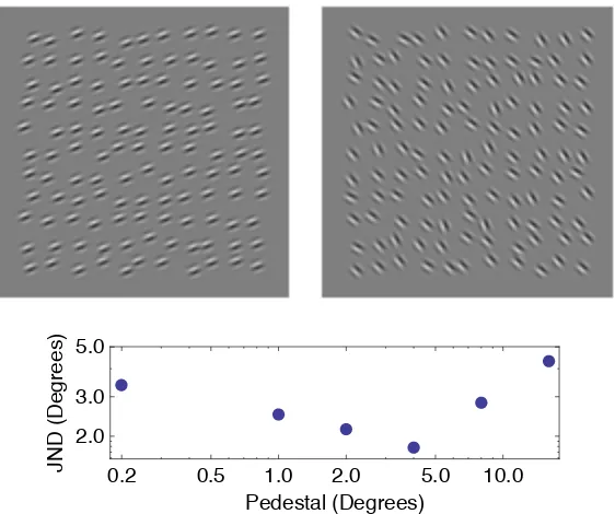
squelched its own noise. To test this possibility, they measured how well observers could discriminate between two textures, whose otherwise parallel elements were tilted with different amounts of Gaussian noise.

Figure 2a shows an example of their stimuli. Observers had a two-alternative, forced-choice (2AFC): they were shown two textures, and asked to select the one having greater variance. This variance was manipulated until observers were responding with an accuracy of 82%.

The horizontal position of each point in Figure 2b shows the standard deviation of orientations in the less-variable or “pedestal” texture. The vertical position of each point shows how much greater the standard deviation of the other texture needed to be for MM to identify it with 82% accuracy. This is the JND or just-noticeable difference in standard deviation. The JND’s form a dipper-shaped function of pedestal magnitude. That is, as the pedestal increases from zero, the JND’s first decrease and then increase. This result may seem counter-intuitive, but dipper

functions of this general shape, with a “dip” in the middle and a “handle” on the right, are ubiquitous in contemporary psychophysics. The historical review that follows should help to steer interested empiricists away from particularly contentious issues.

* _{A referee thought it important that I highlight the fact that “Morgan et al” includes}

Figure 2: Example stimuli and results from Morgan et al. (2008). The observer’s two-alternative, forced-choice (or 2AFC) task was to report which of two images had higher variability in orientation. In the example (a), there is zero variability in the image on the left. Orientations on the right were sampled from a Gaussian

distribution with an 8-deg standard deviation. Each point in (b) shows observer MM’s (82% correct) JND in standard deviation.

Weber’s Law

Dipper functions are a subset of those functions that describe the relationship between a baseline magnitude ,* and a just noticeable increment

€

ΔIJND. An even simpler

relationship, attributed to Weber (by Fechner 1860/1912), can be written

€

ΔIJND I=k, (2)

where the “Weber fraction”

€

k does not vary with . So much has been written about Weber’s Law (and the “near-misses” thereto) that I feel unable to add anything

intelligent on the topic. The reader is directed to Chapter 1 of Laming (1986). Chapter 2 contains an unbeatable review of the psychophysical methods appropriate for obtaining Weber’s Law.

Conventional psychophysical methods (e.g. 2AFC) constrain the possible relationships between and

€

ΔIJND. A recent discussion of these constraints can be

found in Doble, Falmagne, and Berg (2003) and Iverson (2006a, 2006b). All are satisfied by Weber’s Law.

Luminance discrimination

* _{I stands for intensity, which has a very precise physical definition. On the other}

hand, both the word “magnitude” and Weber’s Law are much more general.

1.0 0.5 2.0

0.2 5.0 10.0

5.0

2.0 3.0

Pedestal (Degrees)

JND

(Degrees

)

!

I

!

I

!

Following many previous authors, Bartlett (1942) obtained Weber fractions for detecting luminance increments on a steady background. He obtained different Weber fractions when

€

I and

€

I+ΔI were presented on a background

€

≠I. Like many other

authors, Bartlett used the same symbol to denote both an arbitrary increment and a just noticeable one. I will reserve

€

ΔI for the former and

€

ΔIJND for the latter.

Following Bartlett (1942), Cornsweet and Pinsker (1965) distinguished between 2AFC detection of luminance increments on a steady background and 2AFC discrimination of luminance “pulses” on a dark background. Only the latter type of experiment produced dipper-shaped plots of

€

logΔIJND vs

€

logI (cf. Blackwell, 1963).

These dipper functions had long, straight handles with a gradient of 1. Thus Weber’s Law held for large values of

€

I, i.e. whenever the pulses could be easily detected.

Plotting tip: I recommend using coordinate systems in which one log unit has the same length vertically and horizontally. This makes it relatively easy to visually estimate the handle gradient and thus the validity of Weber’s Law for large values of

€

I.

Variance discrimination

The very first dipper function was published by Raab, Osman, and Rich (1963a). The task was to detect brief increments in the amplitude of continuous auditory noises of various intensity. Since loud background noises usually make it hard to hear quiet increments, their effect is often called masking. Raab et al coined the term “negative masking” to describe how the power of the just-detectable increment decreases as the background noise increases from zero. The funny thing is that Raab et al didn’t even do the experiment. The data were originally published by Miller in 1947.

Miller (1947) plotted the just-detectable increment in power, instead of the power of the just-detectable increment, and consequently did not get any negative masking. The distinction is important, so I will explain why no increase in the just-detectable increment in power can actually be a decrease in the power of the just-detectable increment.

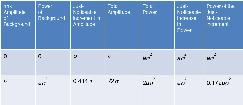
A bit of physics might be useful here. Random fluctuations in pressure sound like noise. The power of an auditory noise is proportional to the variance in pressure. The amplitude of an auditory noise is typically expressed as the root-mean-squared (RMS) pressure, i.e. amplitude is proportional to the square-root of power. Finally, a quantity we will discuss later is energy. To get any signal’s energy, you need to integrate its power over both its extent (in time for auditory signals; in space and time for visual ones) and its bandwidth.

Now, consider the case of detection. That is, when there is no background noise. That is what the “0” means, under “Power of Background,” in the first row of Table 1. When the power is zero, the amplitude is also zero. Without loss of

generality, we can assume that a short burst of noise requires an RMS amplitude of

σ in order to be just detected in total quiet. The symbol σ is typically used to denote

rms Amplitude of Background Power of Background Just-Noticeable increment in Amplitude Total Amplitude Total Power Just-Noticeable increase in Power

Power of the

Just-Noticeable increment

0 0 σ σ _aσ2 _aσ2 _aσ2

σ _aσ2 0.414σ √2σ _2aσ2 _aσ2 _0.172aσ2

Table 1: Negative masking with a constant JND in power.

The total amplitude of a just-detectable noise-burst is thus

€

0+σ=σ, and

since power is proportional to pressure variance, the total power at detection threshold is some constant a, times

€

σ2. To calculate the just-noticeable increase in power, we

subtract the background power from this value (

€

aσ2−0=aσ2), and the power of the

just-noticeable increment is the same constant a, times the same variance

€

σ2.

Moving on to the bottom row of Table 1, we now consider a just-detectable background. Its amplitude, as we have already assumed, will be at least approximately identical to that of the just-detectable noise-burst, σ, and its power is thus

€

aσ2.

Here is where it gets interesting. Assume that this very faint background produces no change in the just-noticeable increment in power. This is what Miller (1947) reported. Previously, we had a just-noticeable increase in power of

€

aσ2, so we

will have a just-noticeable increase in power of

€

aσ2 here too. The total power is the

power of the background plus the just-noticeable increase in power, so that is

€

aσ2+aσ2=2aσ2. Since the total power must be a times the total amplitude squared,

the total amplitude must be

€

2σ. The just-noticeable increment in amplitude is the

difference between the total amplitude and that of the background alone. So that is

€

2σ − σ =

(

)

just-noticeable increment. It is simply is a times this value squared:

€

a

(

)

noise.

The preceding example shows why Raab et al (1963) seemed to get “negative masking” when they re-plotted Miller’s (1947) data as the power of the

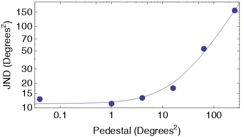
The answer appears in Figure 3. These are the same data as Figure 2, replotted in terms of orientation variance.* In this case, there is almost no evidence of any “negative masking.” The take-home message from this exercise is that, in some cases, negative masking can disappear with an alternative description of stimulus magnitude.

Figure 3: Re-plotted results from Morgan et al (2008). Here, the vertical axis

describes the JND in orientation variance. The solid curve illustrates the performance of a two-parameter observer, whose otherwise-ideal decision is based on a limited number (19) of Gaussian-noise-perturbed (

€

σ =4.4°) samples in each image. These

two parameter values minimize the rms error in log degrees2 _{(cf. Morgan et al., who}

maximized the likelihood of their psychometric data).

Green (1960a) formulated the ideal observer for detecting various signals. He showed that when the signal is a sample of noise, the ideal observer is an energy detector. It is clear from his Equation 7b that Weber’s Law is a consequence of this optimal detector for a noise signal.

Human observers are not ideal for a variety of reasons. Typically, they are inefficient. This means they are unable to utilise all of the available information when making a decision. For example, when estimating signal variance, human observers must rely on a limited sample, and that sample may get corrupted by sensory noise. I fit a noisy, inefficient version of Green’s (1960a) ideal-observer model to Morgan et al’s (2008) discriminations of orientation variance. There are two free parameters in this model: the standard deviation of the putatively Gaussian noise that corrupts each estimate of orientation and the number of Gabor patterns whose orientations MM estimated in each texture, i.e. his sample size. The fit is shown in Figure 3.

One conclusion to draw from this high-quality fit is that acuity for variance is best described in terms of variance. Maybe that isn’t very surprising, but as will be discussed below, the appropriate scale for other acuities is not always this obvious. Note here that I am using the word “acuity” in its most general sense. It refers to an observer’s sensitivity for fine detail in the size or strength of some stimulus.

Before turning away from the dipper function for orientation variance, I must mention its similarity to the dipper function for blur discrimination (Watt & Morgan 1983). Morgan et al (2008) noted that just as the sum of two independent sources of

* _JND

Fig. 3 = (JNDFig. 2 + PedestalFig. 2) 2 – PedestalFig. 22

0.1 1 10 100

10 100

50

20 30

15 150

70

Pedestal (Degrees2)

JND

(Degrees

noise (e.g. that in the stimulus and that intrinsic to the visual system) can be

determined by convolving their Probability Density Functions (PDF’s), the combined effects of stimulus and intrinsic blurs can be determined by convolving their

individual point-spread functions. Thus the dipper function for Gaussian blur and the dipper function for orientation variance may be modeled by the same noisy observer.

Amplitude discrimination: Appropriate description

Although Raab et al were the first to use the term “negative masking,” it was Green (1960b) who first reported evidence of it, when he measured how easy it was to detect changes in the amplitude of a pure tone. Specifically, a faint tone was easier to detect when it was presented in phase with another, near-threshold tone of the same

frequency and duration. Pfafflin and Mathews (1962) introduced the term “pedestal” to describe Green’s facilitating tone.* Although the energy detector is not ideal for discriminating between tone amplitudes, Pfafflin and Mathews found Green’s results with faint tones were nonetheless consistent with its behavior.

Due to the energy model’s success in explaining Green’s (1960b) negative masking and psychometric slopes, Raab et al (1963b) argued that discrimination results should be described and plotted in terms of energy differences, rather than amplitude differences. Like Raab et al, Laming (1986, page 13) reviewed the problem of appropriate scale for dipper functions, but he came to the opposite conclusion. The argument for amplitude appears in his Chapter 4. One reason is that amplitude

frequently has a more “natural” unit of measurement (cf. degrees2).

Weber’s Law itself can supply an even better reason. Fechner (1860/1912) and many others believed that the intensity of sensory experiences increased in proportion to the ratio

€

ΔI I. It follows that the accumulation of sensory noise should produce Gaussian perturbations in these intensities. Thus, psychometric functions of this ratio should resemble the Gaussian CDF, i.e.

€

ψ Δ

₍

₎

₍

₎

€

I is easily detected and

€

ΔI is

proportional to an amplitude difference, not a power or energy difference. Of course, Laming did not examine every type of acuity and there may be some exceptions. Orientation variance may be one of these exceptions. We do not know, because Morgan et al (2008) used a staircase procedure to quickly estimate JND’s.

Methodological tip: Try to collect complete psychometric functions, so that their shapes may be compared with the Gaussian CDF.

Amplitude discrimination: Shape of the dipper function

* _{Leshowitz, Taub, & Raab (1968), who replicated Cornsweet and Pinsker (1965),}

confused the terminology by introducing a hybrid paradigm, with pulsed signals of intensities

€

I and

€

I+ΔI added to a “pedestal” of intensity

€

Hanna, von Gierke, & Green (1986) obtained dipper functions for 2AFC amplitude discrimination of short tones. When these tones were presented against a background of auditory noise, their data were like those of Morgan et al (2008): negative masking did not survive the transformation into energy differences.* _{However, when the tones}

were presented against a quiet background, Hanna et al found that negative masking survived the transformation. Implications of this result appear below.

Craig (1974) obtained a dipper function for discriminating amplitudes of vibrotactile stimulation. The handle had a gradient of 1. I re-plotted his JND’s as energy differences, and found that one point still strongly suggested negative masking.

A huge number of studies report dipper functions for the detection of contrast increments in sinusoidal luminance gratings. Campbell and Kulikowski (1966) were the first. They used the method of adjustment and plotted their dipper function upside-down with respect to current conventions. The handle of their dipper function had a gradient of -1, seemingly consistent with Weber’s Law.

Nachmias and Sansbury (1974) published the next major study on contrast discrimination. They used the 2AFC paradigm. I transformed their data into energy differences, and found only one point that still suggested negative masking. This data point may be an outlier. Legge and Foley (1980) conducted a much larger study using a similar methodology, but none of their dipper functions suggest negative masking when re-plotted as terms of energy differences. Legge himself was one of the first to realize how the dipper function for contrast changes shape when replotted as a dipper function for contrast energy (Legge & Viemeister, 1988). However, even in today’s literature, most contrast dippers appear as Nachmias and Sansbury’s did: JND’s in contrast vs. pedestal contrast.

Nachmias and Sansbury’s (1974) study begat an even more heated controversy, because unlike Campbell and Kulikowski (1966) the handle of their dipper function had a gradient < 1, seemingly inconsistent with Weber’s Law. Kulikowski and Gorea (1978) responded with evidence suggesting that Campell and Kulikowski’s otherwise irreproducible finding could be attributed to contrast

adaptation, a by-product of the method of adjustment. However, Legge (1981) failed to replicate Kulikowski and Gorea using 2AFC. He speculated that their results (and Campbell and Kulikowski’s) might have been due to some other artifact of the method of adjustment.

Explaining the dip: Sensory thresholds

Now it is time to consider those cases in which negative masking does not disappear when the data are plotted in terms of variance (or power or energy) differences. As noted above, Cornsweet and Pinsker (1965) obtained dipper functions when

€

I was the luminance† of a flash against a dark background, and

€

ΔIJND was a just-noticeable

* _{There is actually evidence for a tiny bit of negative masking in Figure 3. The JND}

for a 1-deg2 pedestal is slightly less than those for the 0 and 4- deg2 pedestals.

increment in that luminance. The ideal discriminator will consequently produce a monotonically increasing curve like the one in Figure 3. Something else must have been responsible for the dip.

Crozier (1950) speculated that the retina might absorb some quanta, which could not be used for vision until yet more were absorbed. In this

“photosensitization” process, the retina acts like a kind of teapot, but light goes into it instead of water. Only when it is already “full” does additional light produce any output. This sensory threshold theory predicts a negative masking even when

€

ΔIJND

represents an energy difference. Morgan et al’s (2008) experiment was designed to reveal the existence of an analogous threshold for orientation variance. Although the evidence of negative masking in Figure 3 is meagre, a significantly better fit can be made to the raw data summarized therein, by bolting a sensory threshold onto the otherwise merely noisy and inefficient observer. (Details appear in Morgan et al.)

As the name suggests, high-threshold models have sensory thresholds so high that they prevent observers from ever perceiving visual noise. This type of model can be rejected on the basis of Swets, Tanner, and Birdsall’s (1961) two-response 4AFC experiment. Without visible noise, unlucky guesses are the only way to make errors in a forced-choice experiment. The high-threshold models predict that all 4AFC errors are caused by unlucky guesses. Contrary to this idea, Swets et al found that second responses were more often correct than could be attributed to guessing. Thus, some 4AFC errors must have been due to visual noise.

Green and Swets (1966) identified one low-threshold theory not inconsistent with the extant data. As its name suggests, this theory supposes that visual noise is sometimes visible, and thus causes some forced-choice errors. The rest are caused by unlucky guesses. Although they did not attempt to fit Swets et al’s data with this model, I did (in Solomon 2007a*). The fit wasn’t very good.

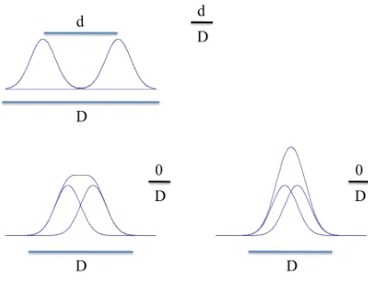
Nonetheless, sensory thresholds might arise naturally in certain situations. One of these is spatial interval discrimination (David Burr, personal communication), where what is measured is the acuity for the distance between two points of light. The idea is that each point gets blurred by the visual system, and that acuity might depend on the ratio of the distance between the peaks of the blur circles to the distance between the far edges of the blur circles. (See Figure 4.) When the points are

sufficiently close, there is zero distance between the peaks of the bur circles, and thus they must be moved farther apart for their separation to be detected. (Dipper functions for this task and a variety of alternative models are discussed in Levi, Jiang & Klein 1990.)

* _{This reference is a tutorial on Signal-Detection Theory. It includes mathematical}

Figure 4: Hypothetical computation of spatial intervals. Each panel shows two Gaussian density functions, each of which represents a blurred point of light, and their sum. If separation acuity depends the ratio of the distance between the peaks in this sum (d) to its overall width (D), then JND’s for large pedestals, which produce bimodal sums, may be smaller than the JND’s for small pedestals, which do not.

Explaining the dip: Intrinsic uncertainty

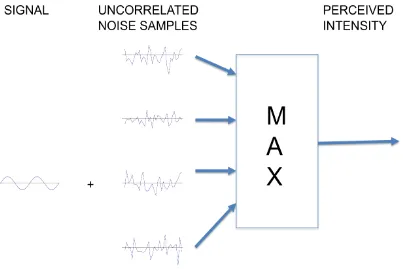
Green (1961) described the intrinsic-uncertainty model of pure tone detection. Tanner (1961) may have published the idea first, but Green actually specified the model. Basically, the idea was that observers monitored a whole bunch of irrelevant channels when trying to detect a weak stimulus. (See Figure 5.) Since these channels played no role in suprathreshold discrimination, detection (i.e. the case where

€

I=0) was

Figure 5: Intrinsic Uncertainty Theory. Observers monitor a whole bunch of irrelevant channels (thousands can be required to fit some data; Pelli 1985) when trying to detect a weak stimulus.

Intrinsic uncertainty is a powerful theory because with just two free parameters it adequately predicts the amount of negative masking, the second-response accuracy in Swets et al’s (1961) 4AFC detection experiment (Solomon 2007a) and the slope of the psychometric function for detection. When plotted on a logarithmic abscissa, this slope is completely determined by the number of irrelevant channels. The theory’s other free parameter is the amount of noise in each channel. Although powerful, intrinsic uncertainty remains unpopular. One reason for this is Watson, Franks, and Hood’s (1972) finding that psychometric functions for detecting pure tones in quiet were even steeper than those for detecting pure tones in noise. Legge, Kersten, and Burgess (1987) replicated Watson et al in the visual domain. They found that the addition of noise, which should not affect intrinsic uncertainty, nonetheless caused the slope of the psychometric function for detection to flatten. Consequently, they rejected intrinsic uncertainty.

Explaining the dip: Non-linear transduction

Taking their cue from Fechner, Nachmias and Sansbury (1974) suggested that JND’s simply reflected the perceived magnitude of a stimulus. Consequently, they inferred an accelerating transducer for small stimulus contrasts. In particular, they modeled the intensity of the “internal effect” as a power function of stimulus contrast, with an exponent between 2.2 and 2.9, depending on the observer. As the pedestal increases, so does the slope of this transducer, and consequently less of an increment in contrast is required for a significant difference in perceived contrast.

Without loss of generality, we can say that the 2.5% stimulus created an internal effect that was

€

Δr greater than that created by a stimulus with 0% contrast. Now

suppose further experimentation reveals that otherwise identical stimuli with 2 and 3% contrasts can be similarly discriminated (i.e. with 75% accuracy in a 2AFC experiment). Thus the 3% stimulus must have created an internal effect that was

€

Δr

greater than that created by the 2% stimulus. Note that a plot of JND vs pedestal contrast would thus suggest negative masking. If we wanted to ascribe this dip to a power-law transducer, we would simply have to find the exponent p, which solves the simultaneous equation

€

0.025p

−0=Δr=0.03p

−0.02p_{. (3)}

In this case,

€

p≈2.5.

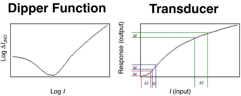
Legge and Foley (1980) also fit their data with a non-linear transducer model; a modification of the version proposed by Stromeyer and Klein (1974). With four parameters, they showed it was possible to describe the entire dipper function (see Figure 6).

Figure 6: Nonlinear transduction. The Transducer shows the relationship between stimulus magnitude (on an arbitrary dimension) and the response of one sensory mechanism. In general, two stimuli can be discriminated if and only if the responses they elicit differ by more than some criterion

€

Δr, Negative masking will happen whenever the sensory response increases faster than the stimulus magnitude. Consider what happens when the pedestal is zero. The JND for detection is

represented as the distance between the two vertical red lines. The vertical blue lines are closer together, thus the JND for small pedestals is smaller. And because the green lines are further apart, the JND for large pedestals is larger.

One-mechanism explanations of the handle

Thus, the simplest explanation of any dipper function is that it reflects the non-linear transduction of stimulus magnitude into a sensory response. However, it could be argued that the transducer isn’t much of an explanation. It is just an alternative way to describe the data.

results, Swets et al (1961) proposed that the variance of sensory signals increased faster than their means. Pfafflin and Matthews (1962) recognised that this increasing noise had the potential to explain why Weber’s Law was at least approximately correct even for amplitude discriminations between non-stochastic stimuli. Non-linear transduction was not necessary.

Legge et al (1987) argued that compressive transduction and increasing noise models were generally equivalent. We could not confidently infer the transducer function from a dipper function, unless we knew the relationship between the sensory response and its variance. And we could not confidently infer the latter relationship from a dipper unless the transducer were known. Catch-22. Legge et al’s argument, however, included certain assumptions about the distribution of sensory noise and the form of psychophysical task, which has left room for more recent attempts to

differentiate between the two ideas. In the words of Georgeson and Meese (2006), “The jury’s still out.” Other significant contributions to this ongoing debate may be found in García-Pérez and Alcalá-Quintana (2007), Gorea and Sagi (2001), Katkov, Tsodyks, and Sagi (2006a,b), Klein (2006), Kontsevich, Chen, and Tyler (2002) and Solomon (2007b).

Multiple-mechanism explanations of the handle

Green (1983) was the first to articulate the suspicion that dipper functions were not necessarily indicative of any simple mapping between stimulus and a single sensory response, however noisy that response might be. He reported the results of a number of experiments, all of which suggest that amplitude discriminations are based on spectral shape (i.e. a “profile analysis” of the output from narrowly tuned channels) whenever possible (cf. Cornsweet and Pinsker’s 1965 “pulses” in the dark and Hanna et al’s 1986 short tones in quiet). In one of these experiments, later adapted for vision by Nachmias (1993), the intensity of a noise masker varied from interval to interval (i.e. even within a single trial) in the range 30 ± X dB.* The question was, how did the JND for a pure tone depend on X? When each interval was of sufficient length (i.e. 115 ms), the answer was “not much!” As X increased from 0 to 20, the JND increased just 1 dB.

Laming (1986, 1988a, 1988b) proposed that all discriminations are effectively based on the spatiotemporal derivative of stimulus magnitude, rather than stimulus magnitude itself. (Some may be based on the second derivative.) When combined with an early source of Poisson (i.e. increasing) noise (e.g. that in the photon flux), this “differential coupling” effectively turns all magnitude discriminations into variance discriminations, and as shown by Green (1960a), ideal discriminations of variance obey Weber’s Law. Near-misses to Weber’s Law Laming attributed to the recruitment of less-well-tuned channels. Finally, Laming showed how noisy

differential coupling, when combined with early noise and half-wave rectification, can produce an approximate square-law transformation of low-intensity sensory input.

* _{A ten-decibel (dB) increase in the sound pressure level of a noise is a log-unit}

Negative masking is one result of this accelerating transduction. Possibly the most contentious aspect of Laming’s model is his attribution of all suprathreshold visual discrimination errors to quantal fluctuations.

Conclusion

Most dipper functions really aren’t that mysterious. The dip goes away when the data are re-plotted on arguably more appropriate axes. If the dip survives this

transformation, it strongly suggests some kind of sub-optimal processing. Possibilities include a sensory threshold, intrinsic uncertainty, non-linear transduction, or a

combination of the three. Morgan et al (2008) looked, but found only scant evidence for this sub-optimality. The question then remains, why do we not usually notice the visual system’s intrinsic noise? If the visual system does ordinarily squelch it (e.g. by applying a sensory threshold), it certainly does not do so when observers are actively trying to detect a stimulus that has been designed to imitate the noise.

ACKNOWLEDGMENTS

This paper improved, thanks to close reading by David Burr and Charles Chubb. J.A.S. receives support from a Cognitive Systems Foresight Project grant

(#BB/E000444/1) and a grant (#EP/E064604) from the Engineering and Physical Sciences Research Council of Great Britain.

REFERENCES

Bartlett, N. R. (1942). The discrimination of two simultaneously presented brightnesses. Journal of Experimental Psychology,31, 380-392.

Blackwell, H. R. (1963). Neural Theories of Simple Visual Discriminations. Journal of the Optical Society of America, 53, 129 – 160.

Campbell, F. W., & Kulikowski, J. J. (1966). Orientation selectivity of the human visual system. Journal of Physiology,187, 437-445.

Cornsweet, T. N., & Pinsker, H. M. (1965). Luminance discrimination of brief flashes under various conditions of adaptation. Journal of Physiology,176, 294-310.

Craig J. C. (1974). Vibrotactile difference thresholds for intensity and the effect of a masking stimulus. Perception & Psychophysics,15, 123-127.

Crozier, W. J. (1950). On the Visibility of Radiation at the Human Fovea. Journal of General Physiology,34, 87-136.

Doble, C. W., Falmagne, J. C., & Berg, B. G. (2003). Recasting (the Near-Miss to)

Weber’s Law. Psychological Review,110, 365–375.

García-Pérez, M. A., & Alcalá-Quintana, R. (2007). Spatial Vision,20, 5–43.

Georgeson, M. A., Meese, T. S. (2006). Fixed or variable noise in contrast discrimination? The jury's still out…. Vision Research, 46, 4294-4303.

Green, D. M. (1960a). Auditory detection of a noise signal. Journal of the Acoustical Society of America,32, 121-131.

Green, D. M. (1960b). Psychoacoustics and detection theory. Journal of the Acoustical Society of America,32, 1189-1203.

Green, D. M. (1961). Detection of auditory sinusoids of uncertain frequency. Journal of the Acoustical Society of America,33, 897-903.

Green, D. M. (1983). Profile analysis: a different view of auditory intensity discrimination. American Psychologist,38, 133-142

Green, D. M., & Swets, J. A. (1966). Signal detection theory and psychophysics. New York: Wiley.

Gorea, A., & Sagi, D. (2001). Disentangling signal from noise in visual contrast discrimination. Nature Neuroscience,4, 1146–1150.

Hanna, T. E., von Gierke, S. M., & Green, D. M. (1986). Detection and intensity discrimination of a sinusoid. Journal of the Acoustical Society of America,80, 1335-1340.

Iverson, G. J. (2006a). Analytical methods in the theory of psychophysical

discrimination I: Inequalities, convexity and integration of just noticeable differences.

Journal of Mathematical Psychology,50, 271–282.

Iverson, G. J. (2006b). Analytical methods in the theory of psychophysical discrimination II: The Near-miss to Weber’s Law, Falmagne’s Law, the

Psychophysical Power Law and the Law of Similarity. Journal of Mathematical Psychology,50, 283-289.

Katkov, M., Tsodyks, M., & Sagi, D. (2006a). Singularities in the inverse modeling of 2AFC contrast discrimination data. Vision Research,46, 259–266.

Katkov, M., Tsodyks, M., & Sagi, D. (2006b). Analysis of a two-alternative forced-choice signal detection theory model. Journal of Mathematical Psychology,50, 411– 420.

Klein, S. A. (2006). Separating transducer non-linearities and multiplicative noise in contrast discrimination. Vision Research, 46, 4279-4293.

Kontsevich, L. L., Chen, C.-C. and Tyler, C. W. (2002). Separating the effects of response nonlinearity and internal noise psychophysically. Vision Research,42, 1771–1784.

Kulikowski, J. J., & Gorea, A. (1978). Complete adaptation to patterned stimuli: a necessary and sufficient condition for Weber’s law for contrast. Vision Research,18, 1223–1227.

Laming, D. (1988a). Précis of Sensory Analysis. Behavioral and Brain Science,11, 275-296.

Laming, D. (1988b). A reexamination of Sensory Analysis. Behavioral and Brain Science,11, 316-336.

Legge, G. E., & Foley, J. M. (1980). Contrast making in human vision. Journal of the Optical Society of America, 70, 1458–1471.

Legge, G. E. (1981). A power law for contrast discrimination. Vision Research, 21, 457–467.

Legge, G. E., Kersten, D., & Burgess, A. E. (1987). Contrast discrimination in noise.

Journal of the Optical Society of America A,4, 391–404.

Legge, G. E., & Viemeister, N. F. (1988). Sensory analysis in vision and audition. Behavioral and Brain Science,11, 301-302.

Leshowitz B., Taub H. B. and Raab D. H. (1968). Visual detection of signals in the presence of continuous and pulsed backgrounds. Perception & Psychophysics,4, 207-213.

Levi, D. M., Jiang, B. C. and Klein, S. A. (1990). Spatial interval discrimination with blurred lines: Black and white are separate but not equal at multiple spatial scales.

Vision Research,30, 1735-1750.

Miller, G. A. (1947). Sensitivity to changes in the intensity of white noise and its relation to masking and loudness. Journal of the Acoustical Society of America,19, 609-619.

Morgan, M., Chubb, C., & Solomon, J. A. (2008). A ‘dipper’ function for texture discrimination based on orientation variance. Journal of Vision, 8(11):9, 1-8.

Nachmias, J. (1993). Masked detection of gratings: The standard model revisited.

Vision Research,33, 1359-1365.

Nachmias, J., & Sansbury, R. (1974). Grating contrast: Discrimination may be better than detection. Vision Research,14, 1039-1042.

Pelli, D. G. (1985). Uncertainty explains many aspects of visual contrast detection and discrimination. Journal of the Optical Society of America A, 2, 1508-1532.

Pfafflin, S., & Mathews, M. (1962). Energy-Detection Model for Monaural Auditory Detection. Journal of the Acoustical Society of America, 34, 1842-1853.

Raab, D. H., Osman, E., & Rich, E. (1963a). Intensity Discrimination, the 'Pedestal' Effect, and 'Negative Masking' with White-Noise Stimuli. Journal of the Acoustical Society of America, 35, 1053.

Raab, D. H., Osman, E., & Rich, E. (1963b). Effects of waveform correlation and signal duration on detection of noise bursts in continuous noise. Journal of the Acoustical Society of America, 35, 1942-1946.

Solomon, J. A. (2007a). Intrinsic uncertainty explains second responses. Spatial Vision,20, 45-60.

Solomon, J. A. (2007b). Contrast discrimination: Second responses reveal the relationship between the mean and variance of visual signals. Vision Research,47, 3247-3258.

Stromeyer, C. F. III, & Klein, S. (1974). Spatial frequency channels in human vision as asymmetric (edge) mechanisms. Vision Research,14, 1409–1420.

Swets, J., Tanner, W. P., Jr., & Birdsall, T. G. (1961). Decision processes in perception. Psychological Review,68, 301-40.

Tanner, W. P. Jr. (1961). Physiological implications of psychophysical data. Annals of the New York Academy of Sciences,89, 752–765.

Watson, C. S., Franks, J. R., & Hood, D. C. (1972). Detection of Tones in the Absence of External Masking Noise. I. Effects of Signal Intensity and Signal Frequency. Journal of the Acoustical Society of America,52, 633-643.