Optimizing sorting algorithms for the Cell Broadband Engine

Rochester Institute of Technology

RIT Scholar Works

Theses Thesis/Dissertation Collections

5-1-2010

Optimizing sorting algorithms for the Cell

Broadband Engine

Eric J. Offermann

Follow this and additional works at:http://scholarworks.rit.edu/theses

Recommended Citation

Optimizing Sorting Algorithms for the

Cell Broadband Engine

by

Eric J. Offermann

A Thesis Submitted in Partial Fulfillment of the Requirements for the Degree of Master of Science in Computer Engineering

Supervised by

Associate Professor Dr. Muhammad Shaaban Department of Computer Engineering

Kate Gleason College of Engineering Rochester Institute of Technology

Rochester, New York May 2010

Approved By:

Dr. Muhammad Shaaban Associate Professor Primary Adviser

Dr. Roy Melton

Lecturer, Department of Computer Engineering

Mr. Brian Sroka

Thesis Release Permission Form

Rochester Institute of Technology

Kate Gleason College of Engineering

Title: Optimizing Sorting Algorithms for the Cell Broadband Engine

I, Eric J. Offermann, hereby grant permission to the Wallace Memorial Library to reproduce my thesis in whole or in part.

Acknowledgments

I would like to thank my thesis advisor Dr. Shaaban, as well as Dr. Melton for the guidance and support. A special thank you to Brian Sroka and Mark Sroka, of the MITRE

Corporation, for help with code and providing support. I would also like to thank The MITRE Corporation for use of their hardware and network. Thank you Mom and Dad for

Abstract

The quest for higher performance in computationally intensive tasks is and will always be an ongoing effort. General purpose processors (GPP) have not been sufficient for many of these tasks which has led to research focused towards computing on specialty processors and graphics processing units (GPU). While GPU provide sufficient speedups for some tasks, other specialty processors may be better suited, more economical, or more efficient for different types of tasks. Sorting is an important task in many applications and can be computationally intensive when dealing with large data sets. One such specialty processor that has proven to be a viable solution for sorting is the Cell Broadband Engine (CBE).

The CBE is being used as the main platform for this thesis since there are already appli-cations for it that require sorting software. The Cell processor is a general purpose proces-sor that combines one master PowerPC core with eight other vector procesproces-sors connected via a high bandwidth interconnect bus. The user must explicitly manage the communi-cation, scheduling, and load-balancing between the vector processors and the PowerPC processor to achieve the highest efficiency. By optimizing the sorting algorithms for the vector processors, large speedups can be achieved because multiple operations occur si-multaneously.

code for the CBE difficult. Results from previous works have also not been sufficient in providing specific measurements of sorting performance. This thesis will explore the development and analysis of a variety of optimized parallel sorting algorithms written for the Cell processor.

Contents

Acknowledgments . . . iii

Abstract . . . iv

1 Introduction. . . 1

1.1 The Problem Domain . . . 1

1.2 Sorting Algorithms . . . 1

1.3 The Cell Broadband Engine . . . 2

1.4 Sorting on the Cell . . . 3

1.5 Organization . . . 3

2 Sorting Algorithms . . . 4

2.1 Chapter Introduction . . . 4

2.2 Quick Sort . . . 4

2.3 Merge Sort . . . 5

2.4 Bitonic Sort . . . 6

2.5 Heap Sort . . . 7

2.6 Tree Sort . . . 8

2.7 Insertion Sort . . . 8

2.8 Selection sort . . . 10

2.9 Choosing the algorithms . . . 11

3 Vector Processing . . . 12

3.1 Chapter Introduction . . . 12

3.2 Vector Computations . . . 13

3.3 Loop Unrolling . . . 15

3.7 Disadvantages . . . 20

4 The Cell Broadband Engine . . . 21

4.1 Chapter Introduction . . . 21

4.2 Architecture . . . 22

4.3 Power Processing Element . . . 23

4.4 Synergistic Processing Elements . . . 24

4.5 Element Interconnect Bus . . . 26

4.6 Memory and I/O . . . 28

4.7 Vector Processing on the Cell . . . 29

4.8 Known Processor Limitations . . . 30

4.9 Previous Work on the Cell Broadband Engine . . . 31

5 Implementation of sorting algorithms . . . 33

5.1 Chapter Introduction . . . 33

5.2 Hardware . . . 33

5.3 High Level Overview . . . 34

5.4 Program Structure . . . 35

5.5 Detailed Implementation of Framework . . . 36

5.6 Detailed Implementation of Algorithms . . . 38

6 Profiling and Results . . . 42

6.1 Chapter Introduction . . . 42

6.2 Results of Implementations . . . 42

6.3 Comparison of Results To Other Work . . . 46

7 Conclusions and Future Work . . . 49

7.1 Chapter Introduction . . . 49

7.2 Overall Conclusions . . . 49

7.3 Contributions To The Field . . . 49

7.4 Future Work . . . 50

7.5 Future Enhancements - Double Buffering . . . 50

7.6 Future Enhancements - Different Data types . . . 52

List of Figures

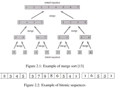
2.1 Example of merge sort [13] . . . 6

2.2 Example of bitonic sequences . . . 6

2.3 Example of a binary split . . . 7

2.4 Example of heap sort . . . 8

2.5 Example of a binary tree used in tree sort . . . 9

2.6 Example of a selection sort . . . 10

3.1 Vector Instruction . . . 14

3.2 Strip Mining . . . 14

3.3 Example of Loop Unrolling . . . 16

3.4 Pipelining example . . . 18

3.5 AsmVis tool . . . 19

4.1 Cell Broadband Engine Architecture [18] . . . 23

4.2 Cell SPE Architecture [2] . . . 25

4.3 128-bit vector capacity . . . 26

4.4 SPE Pipelines [18] . . . 27

5.1 Mercury Computer Systems’ Cell Accelerator Board 2 [4] . . . 34

5.2 Sequence Diagram of Task assignment . . . 37

5.3 Sequence Diagram of SPE DMA . . . 38

5.4 Diagram showing the shuffle for the vectorized merge sort [9] . . . 40

5.5 Combination of Sorting Algorithms - Quick sort then merge sort . . . 41

6.1 Results for sorting 32K integers on the PPE . . . 43

6.2 Results of sorting 32K integers on a single SPE . . . 44

6.3 Results of quick sort for 32K integers on multiple SPEs . . . 44

Chapter 1

Introduction

1.1

The Problem Domain

The quest for higher performance in computationally intensive tasks has driven many chip makers to design multi-core architectures for parallel computing. Theses multi-core chips are needed because General Purpose Processors (GPP) are no longer sufficient for tasks with huge data sets and strict timing requirements. Computations on specialty processors such as Graphics Processing Units (GPU) show much potential, but the cost of such systems is typically much higher and more complex than single chip designs. Multi-core models can often be more economical in terms of cost and some even use less power than many GPU. Sorting is one of the many computationally intensive tasks that require boosts from parallel computing, which is what will be explored in this thesis. The Cell Broadband Engine (CBE) is the target of this research and will run the sorting code on it’s multiple cores to achieve speedups.

1.2

Sorting Algorithms

that the output is a permutation of the input. Many sorting algorithms are classified by both their complexity, memory usage, stability, and number of comparisons. Some of the sorting algorithms that will be considered in this research include, but are not limited to bitonic sort, heap sort, merge sort, and quick sort. Any combination of these may also be used to accomplish the goal of an efficient sorting algorithm for the CBE.

1.3

The Cell Broadband Engine

The Cell Broadband Engine Architecture is a multi-core chip designed by Sony, Toshiba, and IBM in 2005 at the cost of US$ 400 million. The system contains eight vector engines called Synergistic Processing elements (eight of which are available on the system being used for this work), and one main processor called the Power Processor Element (PPE). The PPE sends commands to the Synergistic Processing Elements (SPE) to let them know where to obtain data from, and what to do with the data.

1.4

Sorting on the Cell

Previous research has shown that the CBE is a viable solution for sorting algorithms. Bitonic sort, which is a sorting algorithm designed specifically for parallel machines, is based on repeatedly merging two bitonic sequences to form a larger bitonic sequence. [11] Bitonic sort, as well as the other sorting algorithms will be explained in more detail in Chapter 2. Heap sort is an efficient version of selection sort in which the smallest element is found and swapped with the first element. This is continued until the list is sorted. Merge sort is commonly used to merge two lists of sorted data. It can be useful because some sort-ing algorithms such as Quick sort perform at their worst when the data is partially sorted. Quick sort is one of the fastest known sorting algorithms and will be the main focus in this thesis. It is a divide-and-conquer algorithm in which a pivot is picked and all smaller elements are moved to one side of it, and all larger elements are moved to the other side. This division is repeated recursively to sort both of the sublists.

1.5

Organization

Chapter 2

Sorting Algorithms

2.1

Chapter Introduction

In this chapter, sorting algorithms are introduced and are explored in further detail. A sorting algorithm is a list of instructions that can put a list of objects in order. Since sorting is one of the main components in many applications such as searching and merging, it is very important that they be efficient and as optimized as possible. The output of a sorting algorithm must meet two requirements; that the output must be in nondecreasing order, and that the output is a permutation of the input. Many sorting algorithms are classified by their complexity, memory usage, stability, and number of comparisons. Some of the sorting algorithms that will be considered in this research include, but are not limited to bitonic sort, heap sort, merge sort, and quick sort. Any combination of these may also be used to accomplish the goal of an efficient sorting algorithm for the CBE.

2.2

Quick Sort

Quick sort is a sorting algorithm developed by C. A. R. Hoare that is known to be very efficient for sorting large datasets [8]. The algorithm only requiresØ(nlogn)comparisons to sort n items. However, in the worst case scenario, when the list is already sorted, or partially sorted, the number of comparisons isØ(n2_{). Quick sort uses a divide-and-conquer}

1. Pick a pivot point to start.

2. If any values are less than the pivot, they must come before it. If any values are greater than the pivot, they must go after it.

3. Recursively quick sort each sublist.

The best case scenario for quick sort is when there is a list that has a random order and can perform as fast as Ø(nlogn). The worst case scenario for quick sort is when the list is sorted or partially sorted. When quick sort is performed on an already sorted list, the performance can be as bad asØ(n2_).

2.3

Merge Sort

Merge sort splits the list to be sorted into two equal halves, and places them in separate arrays. Each array is recursively sorted, and then merged back together to form the fi-nal sorted list. This algorithm follows the divide-and-conquer approach by dividing the problem into several subproblems of smaller size, solving the subproblems recursively, and then combines these solutions to create a solution to the original problem. Psuedocode for merge sort is provided below:

1. If the list is of length 0 or 1, then it is already sorted.

2. Divide the unsorted list into two sublists of about half the size.

3. Sort each sublist recursively by re-applying merge sort. 4. Merge the two sublists back into one sorted list.

Neu-Figure 2.1: Example of merge sort [13]

Figure 2.2: Example of bitonic sequences

Merge sort is stable, meaning that it preserves the input order of equal elements in the output. The best case scenario for merge sort is when the data are mostly sorted, where it can perform as fast as Ø(nlogn). The worst case scenario for merge sort is when the data are in reverse order and can take as long as Ø(nlogn). Merge sort is a very common algorithm used in external sorting because it’s worst case performance is the same as the average case performance [14].

2.4

Bitonic Sort

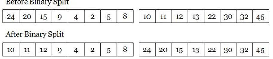
Bitonic sort, which is a sorting algorithm designed specifically for parallel machines, is based on repeatedly merging two bitonic sequences to form a larger bitonic sequence. [11] A sequence of numbers is bitonic sequence if it has at most one local maximum or one local minimum, an example of this can be seen in Figure 2.2.

Figure 2.3: Example of a binary split

A binary split divides the list equally into two. Each item on the first half of the list has a ”partner” which is the process in the same relative position from the second half of the list. Each pair of partners compare and exchange their values, an example can be seen in Figure 2.3. It continues this process recursively, and combines the elements at the end [13]. Bitonic sort can be done inØ(nlogn2)comparisons.

2.5

Heap Sort

Heap sort begins by building a heap out of the data set, and then removing the largest item and placing it at the end of the sorted array. After removing the largest item, it reconstructs the heap and removes the largest remaining item and places it in the next open position from the end of the sorted array. This process is repeated until there are no items left in the heap and the sorted array is full. [13] The worst case scenario for heap sort performs at

Ø(nlogn).

Figure 2.4: Example of heap sort

2.6

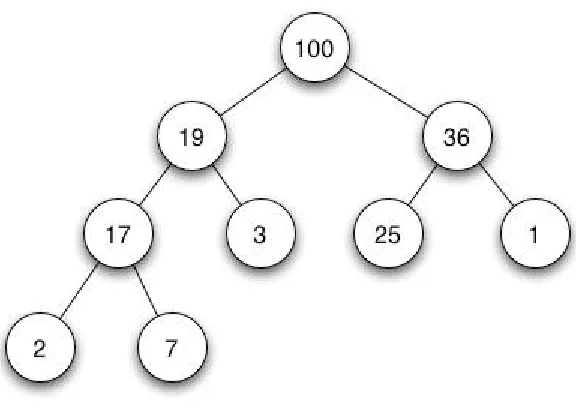
Tree Sort

A tree sort is similar to the heap sort in that it uses the same tree structure with different properties, called a binary search tree. The main feature of the binary tree is that the left subtree of a node must contain only nodes with values less than the node’s value, and the right subtree must contain only nodes with values greater than the node’s value.This property also applies to the subtrees attached to each node. An example of the binary tree can bee seen in Figure 2.5. This type of sorting is useful for sorting streams, as the tree structure can be constructed as the data is received. This eliminates the need to load data into temporary data structure in memory before they can be sorted. This sorting algorithm has a theoretical worst case performance ofØ(nlogn)[17].

2.7

Insertion Sort

Insertions sort is a simple sorting algorithm that is based on comparisons. It is not very efficient for large data sets with even the best case performance as Ø(n2_{). However, the}

Figure 2.6: Example of a selection sort

order of equal elements, and it can sort lists as they are received. Insertion sort sorts a list by selecting one element from the array on each iteration through the loop and moves it to the correct spot in the sorted list. If the algorithm is being used online, meaning it can sort data as it is received, each new element that is received is simply put in the correct location in the already sorted list [12].

2.8

Selection sort

2.9

Choosing the algorithms

Choosing which algorithms to implement was largely based on the requirements for this thesis. The requirements imply that the highest performance is desired for sorting integers in large arrays. The sorting algorithms that seemed to fit the specifications in this case were heap sort, merge sort, and quick sort. Bitonic sort was chosen simply for the reason that this was the algorithm IBM has implemented on the Cell processor and has shown results in their paper [9]. Another reason merge sort was chosen was for the fact that it will be required for the external sorting framework. The algorithms will be mixed and matched for the external sorting in which one sorting algorithm is used across multiple processors and then a separate algorithm may be used to combined the results into a fully sorted list.

Chapter 3

Vector Processing

3.1

Chapter Introduction

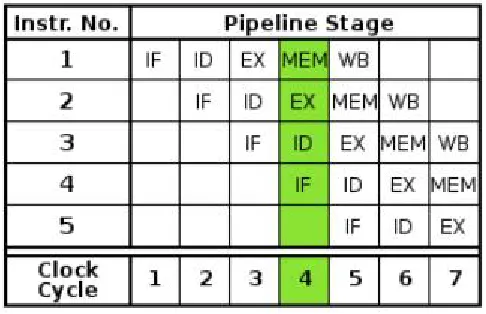
This chapter explores the differences between vector and scalar processors. CPUs typically can operate on only one or two pieces of data at a time, making them scalar processors. Most of the time spent in CPUs is for memory latency since processor speeds have in-creased. Most modern processors use some form of pipelining to increase the throughput, the number of instructions executed in a certain amount of time, of the processors. Pipelin-ing divides the processPipelin-ing of data into separate steps such as the fetch, decodPipelin-ing, execution, memory access, and write back stages. A new instruction can typically enter the fetch stage every clock cycle. In theory, aside from the filling of the buffer, a new result is ready at the other end of the pipeline at the end of each cycle. However, this may introduce hazards into the code and potentially make the performance much harder to predict.

Today, most CPUs implement architectures that feature instructions for vector process-ing on multiple data sets, typically known as Sprocess-ingle Instruction Multiple Data or SIMD. Some common instruction sets include MMX, SSE, and AltiVec. Vector processing tech-niques are also found in video game console hardware, such as the Cell processor, and graphics accelerators.

vector processors can add four numbers to four other numbers, typically in the same amount of time that it took to do one addition operation, or faster. Vector processors typically have a limit to the amount of data that can be operated on at once, this is referred to as the Maximum Vector Length (MVL). A Typical MVL for vector processors can range from 64 to 256 and can be adjusted in some cases using a vector-length register.

3.2

Vector Computations

If a scalar processor needs to operate on 16 or 32 pieces of data, there usually needs to be a loop to perform all of the operations. For a vector processor, this can sometimes be ac-complished with a single instruction. Some vector processors also have special instructions that combine multiple operations into one instruction. For example, a multiply and add op-eration can be combined into one instruction, creating a multiply accumulate instruction. Now there is not only a reduction in the number of times the instruction is executed, there is also a reduction in the number of fetch and decode cycles. An example of how vector instructions compares to a scalar instruction can be seen in Figure 3.1.

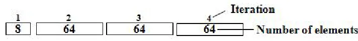
Often times the application requiring vectorization will not fit perfectly into a vector of the respective MVL of a processor. In this case, a technique called strip mining can be used to still vectorize the code without sacrificing a speedup. This is accomplished by operating on only a short piece of the data in the first iteration, being less than the MVL. On the subsequent iterations, the vector length can be readjusted to operate on the full maximum vector length of the processor. An example of strip mining with a maximum vector length of 64 can be seen in Figure 3.2. In this example, the first iteration goes through the loop with only 8 elements and later increases the vector length.

Figure 3.1: Vector Instruction

addressing mode is the vector equivalent of register indirect. This is good for sparse arrays of data or matrices. With the addition of this instruction, the number of programs that are vectorizable increases dramatically.

3.3

Loop Unrolling

Loop unrolling is a technique used in optimizing programs in order to reduce the number of branches and increase the size of the basic block. The larger basic block results in more instructions than can be scheduled or re-ordered by the compiler/hardware to eliminate more stall cycles. This adds an additional layer of parallelism to the already parallel vector instructions. Now not only are there multiple pieces of data being operated on at once, multiple loop iterations happen in just one iteration of the loop.

Loop-Level Parallelism (LLP) analysis must be done on loops that the user wishes to unroll to prevent data dependencies. LLP analysis focuses on whether data accesses in later loop iterations are data dependent on data values produced in earlier iterations. The goal of the analysis is to make loop iterations independent from each other, making them parallel. There are two types of dependencies in loop unrolling, loop-carries and not loop-carried data dependence. A loop carried data dependency means that data produced in an earlier iteration is used in a later one. Not loop-carried data dependence means that there is a dependency within the same iteration of the loop. LLP is done at the source code level since assembly language usually introduces loop-carried name dependence in the registers used in the loop.

Figure 3.3: Example of Loop Unrolling

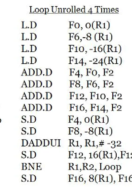
When this loop is unrolled four times for a pipeline, the same instruction from multiple iterations can be executed sequentially to eliminate stalls. For example in the new unrolled code, the first load into F0 is not needed until four cycles later, so the result will be ready by then. Initially, there was a one cycle stall after this instruction, this time was used in the new code to start loading another value into register F6. The same with add and store instructions, stall cycles are replaced with the next iteration of that instruction. Since there is a branch delay slot of one cycle for this example, an instruction can be placed after the branch so that stall cycles are not needed between iterations of the loop. This new code runs through four iterations of the loop in just 14 cycles compared to one iteration in 10 cycles.

instructions are executed. More instructions need to be scheduled for the pipeline, which means more stall cycles can potentially be eliminated. Fewer branches are executed as well as the loop maintenance instructions for decrementing loop counts. However, not all loops can be unrolled. In order for it to be unrolled, all loop iterations must be independent from each other. Also, different registers need to be used in order to avoid hazards.

3.4

Pipelines

Instruction pipelining is used in many processors to increase the number of instructions that can be executed in a unit of time, more commonly known as throughput. Pipelining divides the processing of data into separate steps such as the fetch, decoding, execution, memory access, and write back stages. A new instruction can typically enter the fetch stage every clock cycle. In theory, aside from the filling of the buffer, a new result is ready at the other end of the pipeline at the end of each cycle, allowing the processor to issue instructions as fast as the slowest pipeline stage. However, this may introduce hazards into the code and potentially make the performance much harder to predict.

Figure 3.4: Pipelining example

3.5

Tools

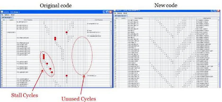
Figure 3.5: AsmVis tool

3.6

Advantages

3.7

Disadvantages

Vector processors also have many pitfalls that in some applications outweigh the advan-tages. Concentrating on peak performance and ignoring start-up costs, strip mining, and other overheads can lead to vector lengths greater than 100 factorial needed to even just match the performance of the scalar code. Increases in vector performance without compa-rable increases in scalar performance proves Amdahl’s Law [1]. The high cost of traditional vector processor implementations such as the Cray supercomputers sometimes cannot be afforded. Another pitfall seen in vector processing is adding the vector instruction support without providing the needed memory bandwidth and low latency to support them. Tradi-tional vector processors such as supercomputers have been abandoned in high performance computing because of these disadvantages, for lower-cost clusters that use multiple general purpose processors.

Chapter 4

The Cell Broadband Engine

4.1

Chapter Introduction

The Cell processor is a chip multiprocessor designed and produced by three manufacturers starting in 2001: Sony, Toshiba, and IBM, sometimes referred to as STI. The processor was created as a solution for general purpose computing applications in many different prod-ucts and fields. The processor was first produced as 65-nm technology, but was advanced in early 2009 to the 45-nm technology, which consumes less power. Although the proces-sors’ claim to fame is as the processor inside Sony’s Playstation 3, it is also used in many scientific applications, as well as HDTVs and HD cameras. These applications all require very high computational efficiency, which the Cell processor delivers [5].

4.2

Architecture

According to Amdahl’s Law, all systems are limited by their slowest components [1]. The Cell Broadband Engine was designed in such a way that it would not have any slow compo-nents. Because of this fact, the architecture and all of its components are very complex, but well thought out. The CBE is made up of a Power Processing Element (PPE), eight Syner-gistic Processing Elements (SPEs), an Element Interconnect Bus (EIB), a Direct Memory Access Controller (DMAC), two Rambus XDRAM memory controllers, and a FlexIO in-terface. A diagram of the Cell architecture can be seen in Figure 4.1.

The Power Processing Element is a PowerPC that is responsible for managing the com-munication, scheduling, and load-balancing of all tasks performed on the processor. Com-munication and scheduling are not automatically performed by the PPE itself, the devel-oper must specify how to send information across the chip as well as where to send it to and when to do it. The eight vector processing SPEs are slave processors to the PPE. These SPEs are capable of performing complex math very quickly and returning data to the PPE over the EIB. The EIB connects all elements of the processor providing a twelve step ring within the Cell. The Memory Interface controller allows all elements to fetch data from main memory in XDR RAM. The Rambus FlexI/O allows all elements to communicate with I/O devices that may be connected to the processor.

• Observed clock speed: Typically 4 GHz or 3.2 GHz

• Peak performance (single precision): 256 GFlops

• Peak performance (double precision): 26 GFlops

• Local storage size per SPU: 256KB

• Area: 221 mm

• Technology 90nm SOI

Figure 4.1: Cell Broadband Engine Architecture [18]

4.3

Power Processing Element

The Power Processing Element, or PPE, is based on both PowerPC and POWER processor architectures and is a two-way multi-threaded core that acts as the master for the eight SPEs on the chip. Since it is very similar to the 64-bit PowerPC chip, it runs normal operating systems and most of the applications on the system. Also, since the PPE lacks computational power and efficiency, it is mainly responsible for controlling the operation of the SPEs to which all of the work is offloaded. It controls them by loading programs as contexts that run on each core. The PPE can then wait for a response from all SPEs that have been given work. Once it has heard back from all SPEs, it either can send out more computations to be done, or can end the program.

su-chosen as opposed to the CISC architecture because of the simplicity which requires less circuitry and consumes less power. The performance for applications with a lot of branch-ing can be unpredictable, but is compensated for with the dual threadbranch-ing capability and the high clock speeds of up to 4 GHz. The Cell is also equipped with IBM’s hypervisor technology which allows it to run two operating systems simultaneously: one normal OS and one real time OS.[6]

4.4

Synergistic Processing Elements

The eight SPEs, sometimes referred to as SPUs, contained in the chip are self contained in-order vector processors. Each vector engine has a small local store of 256 kilobytes instead of having a cache. Not having a cache makes them slightly harder to program, but reduces the complexity of the hardware and increases the speed of the chip. Most processors spend a majority of their time waiting for memory to load into cache. The entire program, or context, that was sent from the PPE to the SPE, including the data to be processed must fit into this local memory. Each core can then fetch the data it needs from RAM via Direct Memory Access (DMA) commands. Each SPE context contains information specific to that SPE and the particular task it was assigned. Each SPE also contains 128, 128-bit registers, which can be used for temporary storage as well as by the compiler for loop unrolling. The SPEs each have two pipelines which each run different instructions to optimize the operations further and increase throughput. A diagram of the contents of a SPE can be seen in Figure 4.2.

The vector processors can execute multiple operations simultaneously with a single in-struction, hence Single Instruction Multiple Data, or SIMD for short. This capability gives the Cell processor its computational power. With these special SIMD instructions, oper-ations can be performed on multiple data simultaneously, yielding high speedups. Figure 7.2 lists how much data can be contained in each 128-bit vector.

Figure 4.3: 128-bit vector capacity

double precision floating point operations, integer multiplies, logical operations, element rotates, and byte operations such as sums and averages. The odd pipeline handles loads and stores, branches, shuffle bytes, quadword rotates, shifts, gathers, and masks. Figure 4.4 shows the two pipelines and the channels of each. The SFS is the Even Fixed-Point Unit, SLS is the SPU Load/Store Unit, SCN is the SPU Control Unit, SSC is the SPU Channel/DMA Unit, SFP is the SPU Floating Point Unit, and SFX is the SPU Odd Fixed-Point Unit.

4.5

Element Interconnect Bus

Although unrealistic because of the arbitration unit, the theoretical maximum for the EIB then would be 96 bytes per clock since it runs at half the system clock speed.

Transactions move in steps around the EIB. Since there are twelve elements connected to the ring, there are twelve steps. Transactions do not move more than six steps in any direction to a destination; if the number of steps is greater than six, the transaction must go in the other direction to reach its destination. The number of steps has no significant impact on the transfer latency, besides the fact that they will reduce available concurrency.

4.6

Memory and I/O

The Memory Flow Controller (MFC) controls data transfers and synchronization between main storage and local storage or between two local stores. Commands which describe the transfer to be performed control the MFC. The purpose of the MFC is to perform the data transfers as fast and as fairly as possible to maximize overall throughput.

In order to transfer data, a MFC Direct Memory Access (DMA) command must be used. These commands are translated into DMA transfers between the main storage domain and the local storage domain. The MFC can support multiple DMA transfers at the same time as well as processing multiple MFC commands. The MFC provides this support by queuing the commands. There is one queue for each SPU and one queue for all the other devices.

The MFC provides two types of interfaces: one to the SPUs and another to all other devices. The SPUs use a channel interface to control the MFC. Code running on an SPU can access only the MFC SPU command queue for that particular SPU. Everything other than the SPUs controls the MFC by using memory-mapper registers. Any processor or device in the system can control the MFC and issue MFC proxy command requests on behalf of the SPU [10].

256MB of XDR, multiple gigabytes can be interfaced to each processor through this mem-ory interface controller.

The I/O interface is called FlexIO and is also made by Rambus. It has five 8-bit wide inbound channels going into the cell and seven outbound channels. The FlexIO has a theoretical peak bandwidth of 62.4 GB/s at 2.6 GHz, which can be clocked independently. The reason for using Rambus technology is because of the synchronization technology it invented called ”FlexPhase.” This technology allows signals to come in at different times, which reduces the need for wires to be exactly the same length. This characteristic saves a lot of development time and simplifies the layout of the boards [?].

4.7

Vector Processing on the Cell

For the Cell processor, the MVL is 128 bits, so depending on the data type, up to sixteen pieces of data can be operated on at once.

During some operations, loss of precision can occur unless properly handled. For ex-ample, on the Cell processor, when multiplying two integer vectors, two instructions need to be used; a multiply even and a multiply odd. The multiply even multiplies all of the even quad words in the vector, (e.g., 0, 2, 4, etc.) and the odd multiplies the odd elements. The result is the creation of two new vectors of larger data types, which in turn means fewer elements can be stored per vector.

4.8

Known Processor Limitations

A known issue with vector processors is that not all applications vectorize well, or are inherently scalar algorithms. This usually means that it is not possible to do more than one operation at a time. Another issue common in developing larger systems is that the code becomes very complex and can often be hard to follow, even by the developers them-selves. Small local stores prove to be a problem in some instances, but can be overcome by using the XDRAM via DMA since the bandwidth on the EIB is very high. One major programming construct that causes significant run time penalties on the Cell are conditional statement, which are if/else statements. In order for the Cell to run efficiently, these must be converted into select logic, which make decisions based on values stored in vectors.

4.9

Previous Work on the Cell Broadband Engine

Sorting algorithms have been studied extensively since the inception of the computer sci-ence discipline [9]. Previous research has shown that the CBE is a viable solution for sorting algorithms [9]. The study done by IBM on the Cell Broadband engine explores a new type of sorting algorithm which was tailored to this specific architecture: CellSort. The design is based on different stages of bitonic sorts, in the SPEs, between the SPEs, and on the PPE. All of the processors work together to sort the list of items. The results from this study showed that the CellSort significantly outperformed quick sort for a large number of items sorted on dual 3.2-GHz Intel Xeon processors. Unfortunately code was not provided with the paper.

Sorting on a Cell Broadband Engine SPU was a paper written at the Univeristy of Florida which briefly explored an implementation of merge sort on a single SPE [7]. The paper review various vector operations used on the SPEs as well as providing small portions of code for reference. It is unclear how many SPEs were used across how many processors, so the results obtained in this experiment were not useful. The work did conclude however that optimizations were possible to increase the performance of sorting algorithms on the cell processor [7].

Classification algorithms have also been optimized for the Cell processor in Mateusz Wyganowski’s Thesis Paper. ”In this work, the feasibility of the Cell processor in the use of training Neural Networks and Support Vector Machines was explored. In the Neural Network family of classifiers, the fully connected Multilayer Perception and Convolution Network were implemented. In the Support Vector Machine family, a Working Set tech-nique known as the Gradient Projection-based Decomposition Techtech-nique, as well as the Cascade SVM were implemented” [19].

the complicated nature of programming the Cell processor. Many fear programming this processor because of the learning curve involved with it. Code will be provided with this thesis so that anyone can read it and to gain an understanding of how to manage the commu-nication, scheduling, and load-balancing between the vector processors and the PowerPC processor to achieve the highest efficiency using the given hardware.

Chapter 5

Implementation of sorting algorithms

5.1

Chapter Introduction

This chapter will discuss the approaches taken to sort an array of integers on the cell pro-cessor. A high level overview will be provided and then a more detailed explanation will be provided.

5.2

Hardware

Figure 5.1: Mercury Computer Systems’ Cell Accelerator Board 2 [4]

5.3

High Level Overview

The goal of the implementation was to create a sorting framework and optimized sorting functions that are efficient with respect to both time and space. The program needs to be compact because of the small size of the local storage on the SPEs which must hold both the program and the data that are to be operated on. The smaller the program is, the more data that can be sorted at a time.

The first major part in the implementation development was to create a framework which allows the PPE to communicate with the SPEs. This part was essential to the thesis in that it controlled all communication between the elements in the cell processor. Correct DMA access is vital because data packets must be sized according to the 128-bit alignment required by the EIB. Once the framework was created and tested, the sorting algorithms were put in place to be optimized.

Instead bitonic was benchmarked as a scalar algorithm on the PowerPC Element.

To start developing code, the original three algorithms were implemented on the Pow-erPC to provide a benchmark for future optimizations. Optimizations were made to each of the sorting algorithms incrementally. After implementing the original version of each algorithm on the SPEs, they were converted to use the special vector operations for the SPEs. The first round of optimizations used only vector instructions for the sake of reduc-ing penalties for usreduc-ing scalar operations. The vectors that were used were not full; just the first element contained real data, and the others were filled with zeros.

The second round of optimizations involved fully vectorizing merge sort so that all vectors were full of real data. Quick sort and heap sort were not able to be fully vectorized without requiring significant amount of conditional logic, which incurs significant delay penalties.

After all optimized algorithms were working properly, the next step was to make them scalable. This meant that the sorting could be done across multiple SPEs and then ulti-mately merged back into a sorted list. The idea for this was derived from external sorting [14], in which data sets are too large to be fully sorted in local storage. Quick, heap, and merge sort were all implemented across multiple SPEs, and a specialized version of the vectorized merge sort was used to merge the data back together. This merging could take place either on the PPE or on another SPE, and in this case a SPE was chosen to simulate the worst case scenario when the PPE is busy with another task.

5.4

Program Structure

When developing software for the cell processor, a host linux box is used to write code in a text editor and then compiled using proprietary IBM CBE make files. The user must compile the code on the host machine from the ppe directory. A special make file was used to compile everything from the ppu, spu, and header directories along with the Cell SDK libraries. The complex make file used in this implementation is a proprietary IBM implementation. Once the program is compiled, the user can SSH into the Cell processor and run the program. The OS that the cell processor card is using does not have the same functional features as the linux machine, so it was not good for anything except executing the code.

5.5

Detailed Implementation of Framework

The framework for the sorting application was developed to be simple to use and also to be adaptable to future implementation and modifications. The main program is contained in the ppemain.c file. This sends commands to the SPE and also receives data when they are finished. The storage that the PPE uses is the XDR, so addresses must be passed to the SPEs in order for them to DMA the data they need. The first thing the PPE does is start up all of the SPEs. Once each SPE is up and running, it reports back to the PPE stating that it is ready to perform tasks. The ppemain.c calls the ppecontrol.c to send a message to the SPE based on what operation needs to be performed. The ppecontrol.c then constructs a message based on the specified parameters for that particular operation. The message contains information such as the address of the data in memory, where to put the sorted data once it is ready, how many data blocks will be sent, which SPE it is intended for, as well as profiling information. This message is then sent to the mailbox of the SPE(s) to notify them they have a task to complete. A sequence diagram showing the process of sending tasks to SPEs can be seen in Figure 5.2.

Figure 5.3: Sequence Diagram of SPE DMA

through the MFC. The SPE program calls the speXfers.c function to request data from the MIC. The data are loaded into the local storage address which was provided as one of the parameters to the speXfers.c function. Once the data are in local storage, the SPE can perform the requested operation, which was also part of the original message. The SPE performs the operations and then calls the speXfers.c function again to send the sorted data back to the MIC. The output address for the sorted data was provided in the original message, so this is used to store the sorted data back on the main memory side. Once the data have been written back to the new location, the SPE sends a message to the PPE stating that it has finished the task it was assigned. Before this message is sent, the PPE is waiting for responses from all SPE that it brought on-line. A sequence diagram showing the process of retrieving data from main memory can be seen in Figure 5.3.

5.6

Detailed Implementation of Algorithms

found to be correct and working properly, they were implemented on the SPE side of the framework. The algorithms remained the same for the first step, but commands were added for each type of sort so that the PPE could communicate which operation it wanted the SPE to perform.

Next the sorting algorithms were implemented to be divided up among multiple SPEs. This was done by dividing the total array of data into the desired number of SPEs. The addresses for storing the result also needed to be calculated based on the SPE number. Validation was also created for this step even though the data that were returned did not create a fully sorted list. What was returned were n sorted lists, where n is the number of SPEs that sorted the list. Special attention was required for making sure that all of the addresses were multiples of 128 bits so that there would be no bus errors when sending and receiving data.

Quick sort and merge sort were both optimized for the next implementation. Quick sort was optimized in such a way that the special vector instructions for the SPEs could be used without affecting the outcome or complexity of the algorithm. This was accomplished by inserting each piece of data into its own vector, and filling the rest of the vector with zeros. Although this may seem like a waste, it keeps the algorithm simple for the time being as an intermediate optimized version. A similar optimization was made for merge sort in which each data element was given its own vector padded with zeros. Once these optimizations were completed, they were tested for multiple SPEs and validated. Bitonic sort and heap sort were not optimized because the nature of the algorithms did not offer opportunities for optimizations such as the ones used in quick sort and merge sort. In order to optimize these, a significant amount of conditional logic would need to be used, negating the speedups obtained from the optimizations.

Figure 5.4: Diagram showing the shuffle for the vectorized merge sort [9]

and compared. The first element of the vector with the lower value was removed and a new value was shifted into the last position of that vector. In merge sort, all of the elements contained in the vectors came out sorted, and a new set of vectors was created with the next four integers in the array. Each element in the array was shuffled into a new pattern, compared to the other array, and then shuffled back into a sorted order. An example of this shuffle-compare-shuffle operation can be seen in Figure 5.4.

As stated before not all of the sorting algorithms could be easily vectorized. Heap sort and bitonic sort were implemented in a vectorized optimized version, but did not function properly, nor did they run faster than their scalar counterparts.

Figure 5.5: Combination of Sorting Algorithms - Quick sort then merge sort

and B is the algorithm used to combined the data into a fully sorted list. The combina-tions that were created were Quick-Then-Quick, Quick-Then-Merge, Quick-Then-Heap, Merge-Then-Merge, and Heap-Then-Merge. These were chosen based on the performance of quick sort and merge sort. Heap sort was also run as a trial to see if it would be any better than the others. Figure 5.5 shows an example of the combination of quick sort and merge sort. First the quick sort command is sent out to two SPE processors. When those SPEs are done quick sorting the data, a merge sort command is sent out to a new SPE with the addresses of the results of the other two SPEs. When this SPE is finished merging all of the results together, a message is relayed back to the PPE letting it know the data is fully sorted.

Chapter 6

Profiling and Results

6.1

Chapter Introduction

This chapter will discuss the results of the sorting algorithms that were implemented on the cell processor. The results will be compared to previous sorting algorithms developed for the cell processor. Each of the tests that were done in the results section consist of running the algorithms on data sets of 32,000 integers 1000 times to eliminate startup lag.

6.2

Results of Implementations

The various implementations were written for a PCI express card version of the Cell pro-cessor from Mercury Computer Systems as discussed in the previous chapter. The results obtained from this processor would not necessarily be the same as if the program were run on the Playstation 3.

The results for quick sort, merge sort, bitonic sort, and heap sort running on the PPE are shown in Figure 6.1. Merge sort executed slightly faster than quick sort which was unexpected, but the speed difference was not significant. Heap sort ran longer than both merge sort and quick sort which was expected. Bitonic sort ran significantly longer than all other algorithms because of the embedded loops in the algorithm.

Figure 6.1: Results for sorting 32K integers on the PPE

sort the slowest. These results were expected for the unoptimized scalar versions of the sorting algorithms.

Once the algorithms were scaled to multiple processors, more data points were taken to see what kind of speedups, if any, were possible without optimizing the code for the cell processor. These results for sorting 32 thousand integers using quick sort can be seen in Figure 6.3. The results from the PPE version of quick sort were inserted into the graph to show the speedup. The quick sort across multiple SPEs had an execution time of about 1.5 times faster than that of the PPE code or about 50% faster. The combination of quick sort then quick sort is also displayed on this graph showing the performance degradation when quick sort is used as the secondary sort. This was due to the fact that quick sorts worst case scenario is when the list is already partially sorted. Negative results of quick sort can also be seen in Figure 6.5.

Figure 6.2: Results of sorting 32K integers on a single SPE

Figure 6.4: Results of optimized sorting 32K integers on a single SPE

results of the optimizations can be seen in Figure 6.4.

Once the algorithms and framework were adapted to allow for sorting across multiple SPEs, significant speedups were seen across the board, as expected. Results for sorting across multiple SPEs can be seen in Figure 6.5. The combinations of sorting algorithms are also included in this figure.

quick-Figure 6.5: Results of sorting 32K integers on multiple SPEs with quick sort skewed data

6.3

Comparison of Results To Other Work

The results that were obtained by IBM in the CellSort paper [9] showed a much greater speedup for bitonic sort than was seen in the results for quick sort, heap sort, and merge sort in this thesis. The reason for the difference is both the development effort IBM spent on bitonic sort, and the size of the code used for bitonic sort. Since one of the goals for this thesis was to keep the code small enough that it did not take more space than the main application on the SPEs, the vector optimized bitonic sort developed by IBM does not fit the requirements. The results for CellSort can be seen in Figure 6.7. The results were adapted to be comparable to the results from this thesis since IBM used many different parameters including larger data sets and high numbers of SPEs.

Figure 6.8: IBM’s Results Compared to Thesis Results [9]

executed to obtain the results is not known. Also, the code was not run on the exact same platforms, which could affect run times if other processes are running in the background. For instance, if the code IBM implemented was executed on the Playstation 3 at a clock rate of 3.2 GHz, and these thesis results were obtain at 2.8 GHz on the PCI express version of the cell processor. A side by side comparison of the results obtained by IBM and the implementation for this thesis can be seen in Figure 6.8.

Chapter 7

Conclusions and Future Work

7.1

Chapter Introduction

This chapter will discuss if the Cell processor is a viable option for sorting. Contributions to field of high performance computing will be discussed. It will also go into detail of planned future work on the processor.

7.2

Overall Conclusions

This thesis successfully explored the optimizations of sorting algorithms for the Cell pro-cessor. Results that were obtained met the goals of small code size and efficiency. Results for optimized versions of both quick sort and merge sort showed that they would be viable solutions to the sorting problem. The more likely to be used of the two would be merge sort since it performs better in the worst case than quick sort does. The worst case for merge sort does not require the algorithm to go through more iterations like quick sort does when the list is sorted, or almost sorted.

are passed between processing elements which makes it adaptable and scalable. The code that was created is useful to the cell developer community. It is a base line to start at for sorting and is to be improved and collaborated on. The results of this thesis are valuable to anyone working on the cell processor and also to the community for benchmarking the processor against others. The various combinations of sorting algorithms such as the quick-then-quick algorithm had not been previously explored, along with other combinations discussed in this thesis. This work will also be valuable in comparing with GPU as well as porting into OpenCL.

7.4

Future Work

The code and development done for this thesis will be valuable in projects at the MITRE corporation. Future development of the code will be necessary for integration into current systems. Future enhancements and optimizations are also possible for these efforts. The process of optimization often never stops; there is always one more tweak that can improve the performance or efficiency of the code. Of course there is a diminishing return on in-vestment with optimizations where the gains are no longer worth the time spent obtaining them.

Examples of performance enhancements that will be attempted include double buffer-ing to allow SPEs always to have data to work on, as well as adjustbuffer-ing the framework to allow SPEs to communicate with each other and even exchange data using mailbox mes-sages.

7.5

Future Enhancements - Double Buffering

Figure 7.1: An example of double buffering [3]

while the current data is still being calculated. This is often done to hide high memory latencies. The benefits of this technique will only be seen if there is a balance between the transfer time and the amount of computation done on the SPEs. Ideally, this means that the SPEs would never be stalled waiting for data. If the computations do not last long enough, the latency will still be seen. If however the computations are very long, the SPEs will hardly ever be idle waiting for data. An example of double buffering can be seen in Figure 7.1. In this example, two buffers are used to keep the SPE busy at all times. While buffer 1 is in use computing solutions, buffer 0 is making a request, or ”get” command, for the nest set of data. Once the data from buffer 1 is done being used, it is given the ”put” command to send the data back to memory. At the same time, the next computation starts on buffer 0. The process continues, keeping the SPE busy at all times.

Figure 7.2: 128-bit vector capacity

much larger lists since you cannot have the entire list in the same local store. A better option might be to finishing the merging of sub-sorted lists on the PPE side since it has comparable performance. The downside to this is that while the PPE is sorting, it would not have as much control of the main programs if there are others running on other SPEs.

7.6

Future Enhancements - Different Data types

Bibliography

[1] http://demonstrations.wolfram.com/AmdahlsLaw/. [2] http://www.blachford.info/computer/Cell/Cell1 v2.htm.

[3] http://www.kernel.org/pub/linux/kernel/people/geoff/cell/ps3-linux-docs/ps3-linux-docs-08.06.09/CellProgrammingTutorial/CellProgrammingTutorial.files/image056.jpg. [4] http://www.mc.com/products/boards/accelerator board2.aspx.

[5] http://www.research.ibm.com/cell/home.html. [6] http://www.research.ibm.com/hypervisor/.

[7] S. Bandyopadhyay and S. Sahni. Sorting on a cell broadband engine spu. In Comput-ers and Communications, 2009. ISCC 2009. IEEE Symposium on, pages 218 –223, 5-8 2009.

[8] W.H. Butt and M.Y. Javed. A new relative sort algorithm based on arithmetic mean value. InMultitopic Conference, 2008. INMIC 2008. IEEE International, pages 374 –378, 23-24 2008.

[9] Buˇgra Gedik, Rajesh R. Bordawekar, and Philip S. Yu. Cellsort: high performance sorting on the cell processor. In VLDB ’07: Proceedings of the 33rd international conference on Very large data bases, pages 1286–1297. VLDB Endowment, 2007. [10] Toshiba Corp. Internation Business Machines Corp., Sony Computer

[12] S.Z. Iqbal, H. Gull, and A.W. Muzaffar. A new friends sort algorithm. In Computer Science and Information Technology, 2009. ICCSIT 2009. 2nd IEEE International

Conference on, pages 326 –329, 8-11 2009.

[13] Joseph T. Kider Jr. GPU as a Parallel Machine: Sorting on the GPU, 2005.

[14] Donald Knuth. Te Art of Computer Programming, volume Volume 3: Sorting and Searching. Second edition edition.

[15] Donald E. Knuth. The art of computer programming, volume 3: (2nd ed.) sorting and searching. Addison Wesley Longman Publishing Co., Inc., Redwood City, CA, USA, 1998.

[16] A. Maximo, R. Farias, G. Cox, and C. Bentes. Unleashing the power of the playsta-tion 3 to boost graphics programming. InComputer Graphics and Image Processing (SIBGRAPI TUTORIALS), 2009 Tutorials of the XXII Brazilian Symposium on, pages 45 –58, 11-14 2009.

[17] Daniel Dominic Sleator and Robert Endre Tarjan. Self-adjusting binary search trees.

J. ACM, 32(3):652–686, 1985.

[18] Brian Sroka. Cell BE Software Development and Optimization. Internal MITRE Presentation.