Comparing Hitting Time Behaviour of Markov
Jump Processes and their Diffusion
Approximations
Lukasz Szpruch
∗Desmond J. Higham
†November, 2009
Abstract
Markov jump processes can provide accurate models in many applica-tions, notably chemical and biochemical kinetics, and population dynam-ics. Stochastic differential equations offer a computationally efficient way to approximate these processes. It is therefore of interest to establish re-sults that shed light on the extent to which the jump and diffusion models agree. In this work we focus on mean hitting time behaviour in a thermo-dynamic limit. We study three simple types of reaction where analytical results can be derived, and we find that the match between mean hitting time behaviour of the two models is vastly different in each case. In par-ticular, for a degradation reaction we find that the relative discrepancy decays extremely slowly; namely, as the inverse of the logarithm of the system size. After giving some further computational results, we conclude by pointing out that studying hitting times allows the Markov jump and stochastic differential equation regimes to be compared in a manner that avoids pitfalls that may invalidate other approaches.
Key words: birth and death process, Chemical Langevin Equation, finite differ-ence method, Gillespie Algorithm, mean exit time, square root process, stochastic differential equation, thermodynamic limit.
2000 Mathematics Subject Classification: 60H10, 65J15
∗Department of Mathematics and Statistics, University of Strathclyde, Glasgow G1 1XH,
U.K. E-mail: lukas”at”stams.strath.ac.uk
†Department of Mathematics and Statistics, University of Strathclyde, Glasgow G1 1XH,
1
Introduction
Continuous-time, discrete space Markov jump processes are widely studied as models in the natural sciences [31], especially in population biology [28]. They have also found considerable use in cell biology [4, 17, 18, 22, 32], where a chemical kinetics framework [8, 9, 10, 11, 19, 24] has been adopted. We will use the chemical kinetics terminology and refer to the discrete space Markov process as representing the Chemical Master Equation (CME) modeling regime.
When the population size is sufficiently large, it is reasonable to move upscale from the CME to a stochastic differential equation (SDE). Gillespie [11] shows how this SDE, which we refer to as the Chemical Langevin equation (CLE), can be derived under appropriate modeling assumptions, and more rigorous justification of this type of diffusion limit can also be found [23]. Related issues are also addressed in [13].
Replacing the CME with the CLE typically makes both analysis and simulation more tractable, and the development of multi-scale algorithms that combine ele-ments of both regimes is a highly active research area [2, 3, 4, 5, 30]. It is therefore extremely useful to obtain insights into how accurately the CLE approximates the CME. In the case of first order networks, where reaction rates are linear, the moments of the CME satisfy a closed system of ODEs [6]. Gillespie [10] has shown that for first order networks involving a single species, the CLE correctly reproduces first and second moments of the CLE, but not higher moments in general. This result was generalized in [18], where it was shown that the CLE preserves first and second moments and correlations for any first order network.
Although means, variances and correlations are clearly important, there are, of course, many other senses in which we may judge the ability of the continuous-valued CLE to approximate the discrete-continuous-valued CME. In this work we look at hitting times—how long does it take a population size to reach a specified upper and/or lower bound? Hitting times arise naturally in many stochastic modeling scenarios. For example,
• in a bi-stable gene regulation system, how long will it take to switch between states [33]?
• in an integrate-and-fire model, when is the next firing [27, 29]?
• in mathematical physics, when will a particle cross a potential barrier [7]?
time questions for the CLE can be studied via first-order boundary-value ODEs and corresponding analysis for the CME reduces to problems in linear algebra or sequences and series. In sections 2 and 3 we introduce some background material needed for the analysis, and then in sections 4, 5 and 6 we study the three basic reaction types. In the final section we emphasize how the presence of square roots in the CLE can lead to fundamental issues in analysis, and how focusing on hitting time behaviour avoids possible pitfalls.
2
Background and Notation
We are concerned here with the case of a single species that is involved in one or more reaction. Each reaction, for 1≤j ≤L, is specified in terms of
• the stoichiometric vector, which in our case is a scalar νj ∈ R taking the value −1, 0 or 1, and
• the propensity function, aj(x).
If we let X(t) denote the number of molecules present at time t, then the sto-ichiometric vector is defined so that the effect of the jth reaction is to update the state from X(t) to X(t) +νj. Here, νj = −1 if the jth reaction uses up a molecule and νj = 1 if it creates one. The propensity function has the property that the probability of this reaction taking place in the infinitesimal time interval [t, t+dt) is given by aj(X(t))dt. With this set-up, X(t) becomes an integer-valued, continuous-time stochastic process. If we letpi(t) denote the probability P(X(t) =i), the process may be characterized through the CME, which is the set of ODEs
dpi(t)
dt =
L
X
j=1
aj(i−νj)pi−νj(t)−aj(i)pi(t)
, for j = 0,1,2, . . . . (1)
The CLE is then defined according to the Ito SDE
dy(t) = L
X
j=1
νjaj(y(t))dt+ L
X
j=1
νj
q
aj(y(t))dWj(t), (2)
where the Wj(t) are independent Brownian motions. Here, at each time t, the concentration is represented by the real-valued random variabley(t).
Gillespie [11] showed how the CLE arises naturally as an approximation to the CME under certain modeling assumptions; in particular, the number of molecules in the system is required to be “sufficiently large”. This is intuitively clear, as the CLE uses a real-valued concentration rather than an integer-valued molecule count. Consequently, in comparing the two processes, we would anticipate that the match should be better for large numbers of molecules. We will give results that formalize this principle in the context of hitting times.
3
Hitting Times for Markov Jump and Diffusion
Process
3.1
Hitting time for a Markov Jump Process
At the CME level, the scalar process that we study may be regarded as a Markov jump, orbirth and death process. Introducing discrete states {0,1,2, . . . , M} we may regard states 0 and M as absorbing, and define a birth and death process
Z(t) with birth rates {bi}iM=1−1 and death rates {di}Mi=1−1. This process may be characterized via the infinitesimal description
P (Z(t+h) =i+ 1 | Z(t) = i) = bih+o(h),
P (Z(t+h) =i−1 | Z(t) = i) = dih+o(h),
P (Z(t+h) =i | Z(t) = i) = 1−(bi+di)h+o(h),
with b0 =d0 =bM =dM = 0.
It then follows, see for example, [14], that the linear system
(b1+d1) −b1
−d2 (b2+d2) −b2 . .. . .. ...
. .. ... . ..
. .. . .. −bM−2
−dM−1 (bM−1+dM−1)
U1 U2 U3 .. . .. .
UM−1
= 1 1 1 .. . .. . 1 (3) has a solutionU ∈RM−1 such that U
j gives the expected time for the process to be absorbed into state 0 orM given a starting state Z(0) =j.
molecule count to reach either an upper levelbor a lower levela, starting from an initial number xof molecules. Consequently, the general state iof the absorbing birth and death processZ(t) is identified with a molecule count ofa+iforX(t), and we have b−a = M. To avoid confusion when we consider the analogous hitting times for the processy(t) from the CLE, we introduce the notation
TaX(x) = inf{t ≥0 such that X(t) =a, given X(0) =x},
and for the paira < b,
Ta,bX(x) =T X
a (x)∧T X b (x).
We then note that ETX a,b(x)
for X(0) =x=a+i can be found from Ui in (3).
3.2
Hitting time for Diffusion
In this section we summarize some existing theory concerning hitting times for an SDE. For further details, we refer to [7, 21]. For convenience, we introduce general drift and diffusion coefficients, µ(x) and σ(x), and consider a general scalar Ito SDE with a single Brownian motion
dy(t) =µ(y)dt+σ(y)dW(t).
When they exist, we may then define the scale function
S(x) =
Z x
s(l)dl, (4)
where
s(x) = exp
−
Z x2µ(l) σ2(l)dl
,
and thespeed measure
m(x) = 1
σ2(x)s(x). (5)
We introduce the hitting time for the point a and the paira < b as
Ty
a(x) = inf{t≥0 such that y(t) =a, given y(0) =x} and
Ta,by (x) =Ty
a(x)∧T y b(x).
Next, we define the operatorL by
LV =µ(x)dV
dx +
1 2σ
2(x)d2V
Given a fixed initial conditionx∈(a, b), the probability that y(t) hitsb beforea
has the characterization
P(Tby(x)< Tay(x)) =
S(x)−S(a)
S(b)−S(a).
Similarly,
P(Ty
a(x)< T y b(x)) =
S(b)−S(x)
S(b)−S(a). (6)
Next we letuand wdenote the solutions to the two-point boundary value ODEs
Lu= 0, for a < x < b, u(a) = 0, u(b) = 1,
and
Lw =−1, for a < x < b, w(a) = 0, w(b) = 0. (7) It follows thatw(x) characterizes a mean hitting time,
w(x) =ETa,by (x)
(8)
and we also have
w(x) = 2{u(x)
Z b
x
[S(b)−S(l)]m(l)dl
+[1−u(x)]
Z x
a
[S(l)−S(a)]m(l)dl}. (9)
Finally, we introduce some definitions relating to boundary behaviour.
Definition 3.1. The boundary l is attracting if S(x0)−S(l)<∞ for any x0 ∈ (l, r).
Definition 3.2. Letting
Σ(l) = lim aցl
Z x
b
[S(ξ)−S(a)]m(ξ)dξ, (10)
the boundarylis said to be attainableifΣ(l)<∞, and unattainableifΣ(l) =∞.
Definition 3.3. Letting
M(l, x] = lim
aցlM[a, x] = limaցl
Z x
a
m(s)ds, (11)
3.3
Finite Difference Connection
The linear system (3) may be written in the form
bi+di
2 (Ui+1−2Ui+Ui−1) + (bi −di)
Ui+1−Ui−1
2 =−1, 1≤i≤M −1.
This corresponds to a standard finite difference approximation to the ODE
b(x) +d(x)
2 u
′′(x) + (b(x)
−d(x))u′(x) =−1, u(a) =u(b) = 0,
using a mesh spacing of ∆x= 1; see, for example, [26]. Studying the connection between the discrete linear system and the continuous ODE is the essence of this work. In a numerical analysis setting, the discrete object is regarded as an approximation to the continuous, whereas in our context the opposite is true. However our objective of examining the difference between the two in the large system size, M → ∞, limit is comparable with traditional convergence theory in numerical analysis. A major challenge, however, is that the interval (a, b) is not fixed, and hence the traditional style of error bound, see, for example, [26, Theorem 6.1.3], is not useful. (Equivalently, if we rescale the ODE to the interval 0≤x≤1, then the ODE itself becomes dependent upon M and the coefficients do not have bounded Lipschitz constants.) Indeed, as we will see in section 6, to obtain a positive result in this context it may be necessary to measure the error relative to the (growing) solution size as M → ∞. Related issues arose in the small world analysis of [15, 16].
For this reason, we content ourselves with an investigation of specific simple reactions where the asymptotic behaviour of the discrete and continuous systems can be found and then compared.
4
Production from a source
Perhaps the simplest chemical reaction has the form
∅→k X (12)
4.1
Discrete Process
From a population dynamics viewpoint, the CME for (12) defines a pure birth process, with population-independent birth rate. An infinitesimal description of this Markov process X(t) is
P (X(t+h) =s+ 1 | X(t) =s) =k h+o(h),
P(X(t+h) =s−1 | X(t) =s) = 0,
P(X(t+h) =s | X(t) = s) = 1−k h+o(h).
In this simple setting, the times between successive births are independent ex-ponentially distributed random variables with mean 1/k. This has the following immediate consequence, which could also be proved from the general system (3).
Lemma 4.1. Given integers b > a ≥ 0, for any integer x ∈ (a, b) the discrete state Markov process model for (12) with initial molecule countX(t) =x satisfies
ETX a,b(x)
= b−x
k . (13)
4.2
Diffusion Process
The CLE for (12) has the form
dy(t) =k dt+√k dW(t). (14)
Soy(t) is a Brownian motion with drift.
The following lemma characterizes the mean hitting time.
Lemma 4.2. For any 0 ≤ a < x < b, the CLE (14) with initial condition
y(0) =x satisfies
ETa,by (x)
= 1
k
−e−2x+e−2a
−e−2b+e−2a
−e−2b
2 e
2b
−e2x
+b−x
+
1−−e
−2x+e−2a
−e−2b+e−2a a−x+
e−2a
2 e
2x
−e2a
Proof. The scale function and speed measure have the form S(x) =−e−2x/2 and
m(x) =e2x/k. This gives
Z b
x
[S(b)−S(l)]m(l)dl = 1 2k
−e
−2b
2 e
2b
−e2x
+b−x
and
Z x
a
[S(l)−S(a)]m(l)dl = 1 2k
a−x+ e
−2a 2 (e
2x
−e2a)
,
and the result follows from (9).
We note that unlike the discrete process,X(t), the process y(t) in (14) does not preserve positivity. For example, using the expression for S(x) it follows in (6) that
lim
aց0blim→∞P(T
y
a(x)< T y
b(x)) = lima
ց0blim→∞
e−2b−e−2x
e−2b−e−2a =e
−2x.
This limiting probability, however, is small when the initial state is large, in line with our intuition about the relevance of the CLE.
We wish to formalize a sense in which the two hitting times could be close when there is a “large” number of molecules. For this purpose, we will con-sider an asymptotic regime where the upper limit b tends to infinity and the initial molecule count has the formx =αb∈Z for some fixed α∈(0,1). So the initial data scales linearly with the upper exit level. To keep expressions compact we will also seta= 0, or, where necessary, take the limitaց 0. We will refer to this asymptotic setting as the Large Molecule Count Regime (LMCR).
Theorem 4.1. In the LMCR the mean hitting times in (13) and (15) satisfy
E
TX
0,b(αb)
−ET0y,b(αb)
≤Ce−bmin{2(1−α),α)}, (16)
for a constant C independent of b.
Proof. Setting x=αb∈Z and considering the limit b → ∞, we see in (15) that
ETa,by (αb)
= 1
k
1 +O(e−2αb)
−1
2 +b(1−α) +O(e
−2b(1−α))
+ 1 +O(e−2b(1−α))e
−2αb
e−2a
a−αb+e
2a
2 (e
2αb
−e2a)
and so
ET0y,b(αb)
= 1
k
−1
2 +b(1−α) +O(e
−2b(1−αb)+e−2αb) + 1
2 +O(be
−2αb) .
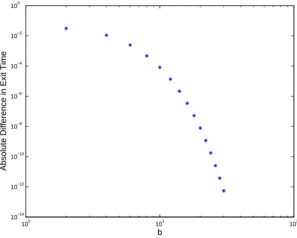
Theorem 4.1 shows that in the LMCR the two hitting times, which grow linearly withb, have an absolute difference that converges exponentially fast. We illustrate this result in Figure 1. Here we took k = 5, a = 0, α = 1
2 and chose values of b
from 2 to 30 in steps of 2. The hitting time discrepancy on the left-hand side of (16) is seen to decay faster than linearly on a log-log scale.
5
Production
In the production reaction
X →c 2X, (17)
new individuals are created at a rate proportional to the current state.
5.1
Discrete Process
In the CME setting, an infinitesimal description for the reaction (17) is
100 101 102
10−14 10−12 10−10 10−8 10−6 10−4 10−2 100
Absolute Difference in Exit Time
[image:10.595.143.440.407.645.2]b
P(X(t+h) =s+ 1 | X(t) =s) =c s h+o(h),
P (X(t+h) =s−1 | X(t) =s) = 0,
P(X(t+h) =s | X(t) = s) = 1−c s h+o(h).
In population dynamics, this corresponds to a pure birth or Yule process [28]. The following result can be obtained from (3) or by simply observing that the times between entering and leaving state s are independently and exponentially distributed random variables with mean 1/(c s).
Lemma 5.1. Given integers b > a ≥ 0, for any integer x ∈ (a, b) the discrete state Markov process model for (17) with initial molecule countX(t) =x satisfies
ETa,bX(x)
= 1
c
b−1
X
s=x 1
s. (18)
5.2
Diffusion Process
The CLE for (17) has the form
dy(t) = c y(t)dt+pc y(t)dW(t). (19)
This is an example of a mean-reverting square root processes, and a unique non-negative solution is guaranteed [25]. The hitting time may be characterised as follows.
Lemma 5.2. For any 0 < a < x < b, the CLE (19) with initial condition
y(0) =x satisfies
E
Ta,by (x)
= 1
c
e−2x−e−2a
e−2b−e−2a
−e−2b
Z b
x
e2l
l dl+ lnb−lnx
+
1−e
−2x−e−2a
e−2b−e−2a lna−lnx+e
−2a
Z x
a
e2l
l dl
, (20)
and for a= 0 we may take the limit limց0 in this expression.
Proof. The scale function and speed measure have the form S(x) =−e−2x/2 and
m(x) =e2x/(cx). Hence,
Z b
x
[S(b)−S(l)]m(l)dl= 1 2c
−e−2b
Z b
x
e2l
and
Z x
a
[S(l)−S(a)]m(l)dl = 1 2c
lna−lnx+e−2a
Z x
a
e2l
l dl
,
and the result follows from (9).
We note that neither (18) nor (20) could be considered as closed form expressions. However, both characterizations are amenable to asymptotic analysis, and we may obtain an analogue of Theorem 4.1.
Theorem 5.1. In the LMCR the mean hitting times in (18) and (20) satisfy
E TX
0,b(αb)
−lim aց0E
Ta,by (αb) ≤
Cb−2, (21)
for a constant C independent of b.
Proof. First we note that the Harmonic series has the asymptotic expansion
n
X
s=1 1
s = lnn+γ+
1
2n +O(n
−2), asn
→ ∞, (22)
whereγ = 0.5772. . .is the Euler-Mascheroni constant [1].
For the CME we have, using (18) and (22)
ET0X,b(αb)
= 1
c "b−1
X
s=1 1
s −
αb−1
X s=1 1 s # = 1 c
ln(b−1) +γ+ 1
2(b−1)−ln(αb−1)−γ− 1
2(αb−1) +O(b
−2)
= 1
c
−lnα− 1
2b +
1
2αb +O(b
−2)
. (23)
Next we introduce the exponential integral
Ei(x) =
Z x
−∞
et
t dt, forx >0,
and note the asymptotic result
Ei(x) =γ+ lnx+o(1), as x→0, (24)
see for example, [1]. At the largex extreme, the expansion
Ei(x) =
ex
x
1 + 1
x +O(x
−2)
follows via integration by parts; see, for example, [20, Chapter 1]. We also have the straightforward identity
Z x
a
e2l
l dl =Ei(2x)−Ei(2a). (26)
Then, using (25) and (26), for any fixed 0< a≤a⋆ we have
e−2αb−e−2a
e−2b−e−2a
−e−2b
Z b
αb
e2l
l dl+ lnb−lnαb
= 1 +O(e−2αb)
×
− 1
2b + lnb−lnαb+O(b
−2)
= −lnα− 1
2b +O(b
−2). (27)
Similarly, we find that
1−e
−2αb−e−2a
e−2b−e−2a lna−lnαb+e
−2a
Z αb
a
e2l
l dl
= e−2αb+O(e−2b)
×
lna−lnαb−e−2a(E
i(2αb)−Ei(2a))
.
Now it follows from (24) that lna−e−2aE
i(2a) is bounded for all small a, and hence we find that
1− e
−2αb−e−2a
e−2b −e−2a lna−lnαb+e
−2a
Z αb
a
e2l
l dl
= e−2αbE
i(2αb) +O(b−2)
= 1
2αb +O(b
−2). (28)
Combining (20), (23), (27) and (28) gives the required result.
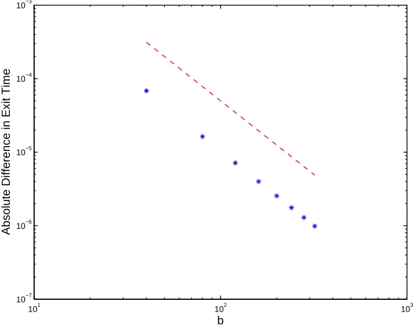
In Figure 2 we illustrate Theorem 5.1 in the case where c = 5, a = 10−3 and
α = 1
2 and the upper limit b ranges from 40 to 320 in steps of 40. The hitting
time discrepancy on the left-hand side of (21), plotted with asterisks, appears to behave linearly on this log-log scale. A reference line of slope−2 is superimposed. A least squares fit to a power law gave a slope of −2.04 with 2-norm residual of 0.02. This suggests that the O(b−2) rate derived in Theorem 5.1 is sharp.
6
Degradation
The degradation reaction may be written
Here a species is undergoing a natural decay process, with a rate that is linearly proportional to the current population size. Intuitively, because of the inherent monotone decrease in the molecule count over time, we would not expect to obtain upper bounds as small as those in Theorems 5.1 and 6.1.
6.1
Discrete Process
In the CME setting, the reaction (29) may be regarded as a pure death process with propensity proportional toX(t). An infinitesimal description is
P(X(t+h) =s+ 1 | X(t) =s) = 0,
P (X(t+h) =s−1 | X(t) =s) =c s h+o(h),
P(X(t+h) =s | X(t) = s) = 1−c s h+o(h).
As for the case of production, the time between entering and leaving states is an exponentially distributed random variable with mean 1/(cs), and all such times
101 102 103
10−7 10−6 10−5 10−4 10−3
Absolute Difference in Exit Time
[image:14.595.143.440.435.670.2]b
are independent. This leads to the following consequence, which could also be derived from (3).
Lemma 6.1. Given integers b > a ≥ 0, for any integer x ∈ (a, b) the discrete state Markov process model for (29) with initial molecule countX(t) =x satisfies
ETX a,b(x)
= 1
c
x
X
s=a+1 1
s. (30)
6.2
Diffusion Process
The CLE for (29) has the form
dy(t) =−cy(t)dt−pc y(t)dW(t). (31)
This is another special case from the class of mean-reverting square root processes, and a unique non-negative solution is guaranteed [25]. The hitting time may be characterised as follows.
Lemma 6.2. For any 0 < a < x < b, the CLE (31) with initial condition
y(0) =x satisfies
ETa,by (x)
= e
2x−e2a
e2b−e2a
1
c
e2b Z b
x
e−2l
l dl−lnb+ lnx
+ [1− e
2x−e2a
e2b −e2a]
1
c
lnx−lna−e2a
Z x
a
e−2l
l dl
. (32)
Proof. The scale function and speed measure have the form S(x) = e2x/2 and
m(x) =e−2x/(cx). We find that
Z b
x
[S(b)−S(l)]m(l)dl = 1 2c
e2b
Z b
x
e−2l
l dl−lnb+ lnx
and
Z x
a
[S(l)−S(a)]m(l)dl = 1 2c
lnx−lna−e2a
Z x
a
e−2l
l dl
,
and the result follows from (9).
We also have
Σ(0) = lim aց0
1 2c
lnx−lna−e2a
Z x
a
e−2l
l dl
and
M(0, x] = lim aց0
Z x
a
m(s)ds =∞,
confirming that zero is an attainable, absorbing boundary.
As in the previous two sections, it is possible to compare mean exit times (30) and (32) in the LMCR to obtain analogues of Theorems 4.1 and 5.1.
Theorem 6.1. In the LMCR the mean hitting times in (30) and (32) satisfy
lim
aց0blim→∞ E
T0X,b(αb)
−ETa,by (αb)
= −ln 2
c . (33)
Proof. From (30), for the CME as b→ ∞ the expansion (22) gives
E
TX
0,b(αb)
= 1 c αb X s=1 1 s = 1
c(ln(αb) +γ) +o(1). (34)
For the CLE, we first consider any fixed value ofa∈(0, a⋆), and look at the limit
b→ ∞. Letting
E1(x) =
Z ∞
x
e−t
t dt, x >0,
denote an alternative type of exponential integral, we may use the asymptotic results
E1(x) =−lnx−γ+o(1), as xց0 (35) and
E1(x) =
e−x
x +o
e−x
x
, as x→ ∞, (36)
see, for example, [1, 20]. We also have the identities
Z b
x
e−2l
l dl=E1(2x)−E1(2b) and Z x
a
e−2l
l dl =E1(2a)−E1(2x). (37)
Then using (36) and (37) in the first term on the right-hand side of (32), we have
e2αb−e2a
e2b−e2a
e2b
Z b
αb
e−2l
l dl−lnb+ lnαb
= e
2αb−e2a
1−e2(a−b) (E1(2αb)−E1(2b))
−e
2αb−e2a
e2b−e2a lnα
= o(1), (38)
For the second term on the right-hand side of (32),
[1− e
2αb−e2a
e2b −e2a ]
lnαb−lna−e2a Z αb
a
e−2l
l dl
= 1 +O(e−2b(1−α)
(lnαb−lna
−e2a(E
1(2a)−E1(2αb))
= 1 +O(e−2b(1−α)
(lnαb−lna
−e2aE1(2a)
. (39)
It follows from (32), (34), (38) and (39) that uniformly ina and for large b,
ETX
0,b(αb)
−ETa,by (αb)
= 1
c γ + lna+e
2aE
1(2a) +o(1)
.
[image:17.595.144.442.436.671.2]Taking the limitaց0 and using (35), we obtain the required result.
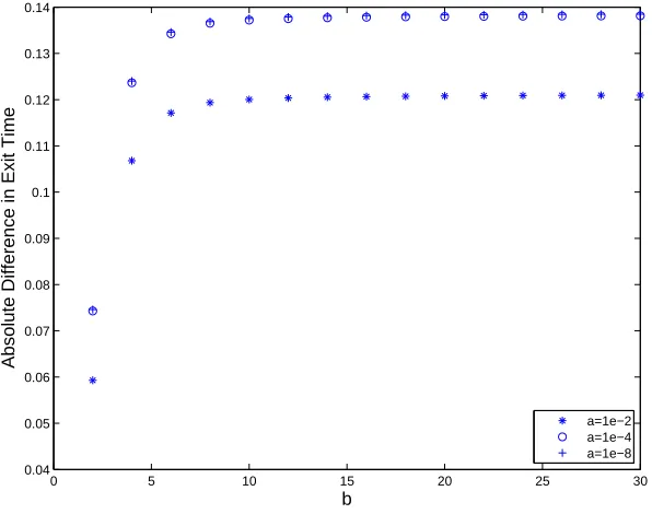
Figure 3 illustrates Theorem 6.1. As for Figure 1 we usedc= 5, α= 1
2 and chose
values ofbfrom 2 to 30 in steps of 2. For the CLE hitting time (32) we took lower limits of a = 10−2, 10−4 and 10−8. We see that as b increases and a decreases, the absolute value of the hitting time discrepancy on the left-hand side of (33) approaches the limiting value ln(2)/5≈0.1386 predicted by the theorem.
0 5 10 15 20 25 30
0.04 0.05 0.06 0.07 0.08 0.09 0.1 0.11 0.12 0.13 0.14
Absolute Difference in Exit Time
b
a=1e−2 a=1e−4 a=1e−8
There is a stark contrast between the results in Theorems 4.1, 5.1 and 6.1. In the first case, the two mean hitting times converge exponentially quickly in the large molecule count limit, in the second case they converge only at a polynomial rate, and in the third case there is a fixed, nonzero limiting absolute error. Since the two hitting times in Theorem 6.1 grow like ln(b) as b → ∞, this lack of convergence in an absolute sense translates into convergence in arelative sense— the ratio of the mean hitting time discrepancy to the actual mean hitting time tends to zero; albeit at a rate of only 1/lnb.
7
Two-way Reactions and General Issues
We begin this final section by briefly discussing difficulties arising with the dif-fusion regime in the case where pairs of reactions are combined. For production from a source (12) and degradation (29), we obtain the system
∅→k X → ∅c (40)
Here, the birth and death rates for the CME areP(X(t+h) =s+ 1| X(t) =s) =
k h+o(h) and P(X(t+h) =s−1 | X(t) =s) = c s h+o(h), respectively, and the corresponding CLE has the form
dy(t) = (k−c y(t))dt+√k dW1−
p
c y(t)dW2, (41)
whereW1(t) and W2(t) are independent scalar Brownian motions.
In this case, where there are two noise sources, the theory in section 3.2 carries through when we interpret σ2(x) in the scale function (4) and speed measure (5) as the sum of the squares of the two diffusion coefficients.
We then find that
s(x) = e2x(k+cx)−4k
c ,
m(x) = exp(−2x) (k+cx)1−4ck
,
S(x) = 24ck−1e−
2k
c (k+cx)−
4k
c (−k+cx
c )
4k c Γ
1−4k
c ,−
2 (k+cx)
c
,
Applying Definition 3.2, we find that zero is an attainable boundary for the SDE (41). Because the first noise term √k dW1 in (41) does not vanish at y = 0, the process may then break down, no longer producing a real solution. Hence, a solution to the CLE only makes sense up to a stopping time defined by the solution reaching zero, and any analysis must acknowledge this fact. The hitting time framework deals with this difficulty in a natural manner.
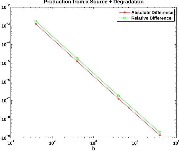
Because direct analysis does not seem possible for (40), Figure 4 reports on a computational test. Here, we took rate constants k = 1 and c = 1. We used a lower limit ofa =b/4 for the exit time, and started withx=b/2 molecules. Val-ues ofb= 4×101,4×102,4×103,4×104, were used. Asbincreases, we are taking a larger system size and, sincea scales likeb, avoiding the case of small molecule counts. The CME and CLE exit times were computed by solving numerically the sparse linear system (3) and the boundary value ODE (7), respectively. We show the absolute and relative difference between CME and CLE exit times on a log-log scale. In this favourable large molecule regime, we observe convergence of the two hitting times—a least squares fit gives a power of −1.99 with a residual of 0.06, suggesting the same rate of b−2 that was rigorously derived in section 5 for a production reaction.
101 102 103 104 105
10−9 10−8 10−7 10−6 10−5 10−4 10−3 10−2
b
Production from a Source + Degradation
[image:19.595.144.434.406.650.2]Absolute Difference Relative Difference
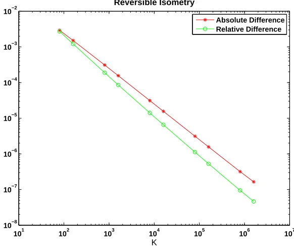
The failure of the CLE (41) to stay nonnegative is not simply a consequence of the additive noise term. To see this, we may consider the reversible isometry
X1 c1X1
⇋
c2X2
X2 (42)
Here, a molecule of species X1 may convert into a molecule of species X2, with propensity proportional to the number ofX1 molecules, and, similarly, a molecule of species X2 may convert into a molecule of species X1, with propensity pro-portional to the number of X2 molecules. In this system, the total number of molecules remains constant. Hence, if we assume that there is a deterministic total of K molecules at time zero then we may write a CLE for X1 alone in the form
dy(t) = (−c1y(t) +c2(K−y(t)))dt−
p
c1y(t)dW1+
p
c2(K−y(t))dW2. (43)
Gillespie [12] uses this example as the basis for comparing steady state distri-butions for the CME and CLE. In the CLE case, Gillespie claims to solve the steady Fokker-Planck equation, and displays analytical solutions for the resulting distribution. Numerical plots are given to show that the steady CME and CLE distributions are close. However, that CLE analysis is done under the implicit assumption that the stochastic process is well behaved for all time and has a well defined steady distribution. Looking at (43) we see that the noise terms do not both switch off at the ‘endpoints’: if y(t) = 0 then the diffusion coefficient
p
c2(K−y(t)) is active and if y(t) =K then the diffusion coefficient −
p c1y(t) is active. Hence, there is no reason to believe that the SDE will remain in the range [0, K]. In fact Gillespie’s conclusion [12, Eq(15)] that forc1 =c2 the steady distribution is normal, contains an inherent contradiction—a normal distribution allows a nonzero probability of molecule counts outside the range [0, K], in which case the process is not well behaved. So, while fully agreeing with the comments in [12] that the CLE is inaccurate in the far tails because this is precisely where the modelling assumptions used to derive the CLE become invalid, we wish to make the further point that this invalidity manifests itself even more seriously through a breakdown in the fundamental existence/uniqueness of the stochastic process. Of course, it is possible to ‘fix up’ the definition of the CLE by introduc-ing reflectintroduc-ing boundary conditions or by takintroduc-ing absolute values inside the square root function, but neither alteration would respect the integrity and elegance of the first principles modelling approach in [11].
104,16×104,8×105,16×105. As in Figure 4, by letting the system size increase and avoiding small numbers of molecules, we observe convergence. In this case a least squares fit for the absolute difference gives a power of −0.99 with residual 0.04, suggesting a rate of K−1.
Our tenet here is that a systematic comparison of the CME and CLE regimes must take account of the fact that the square roots in the diffusion coefficients, which arise perfectly naturally through modelling arguments, cause genuine analytical difficulties. These difficulties can be traced back to the modelling assumptions, and they arise when a species becomes scarce. The approach that we take here of comparing the two regimes in terms of hitting times has the benefit of allowing us to focus on the diffusion process before it breaks down, and it gives a realistic way to address the ‘thermodynamic limit’.
References
[1] M. Abramowitz and I. A. Stegun,Handbook of Mathematical Functions
101 102 103 104 105 106 107
10−8 10−7 10−6 10−5 10−4 10−3 10−2
K
Reversible Isometry
[image:21.595.143.434.403.646.2]Absolute Difference Relative Difference
with Formulas, Graphs, and Mathematical Tables, Dover, New York, 1964.
[2] D. Adalsteinsson, D. McMillen, and T. C. Elston, Biochemical network stochastic simulator (BioNetS): software for stochastic modeling of biochemical networks, BMC Bioinformatics, 5:24 (2004).
[3] K. Ball, T. G. Kurtz, L. Popovic, and G. Rempala, Asymptotic analysis of multiscale approximations to reaction networks, The Annals of Applied Probability, 16 (2006), pp. 1925–1961.
[4] Y. Cao, D. T. Gillespie, and L. Petzold, The slow-scale stochastic simulation algorithm, J. Chem. Phys., 122 (2005), p. 014116.
[5] W. E, D. Liu, and E. Vanden-Eijnden, Nested stochastic simulation algorithms for chemical kinetic systems with multiple time scales, J. Chem. Phys., 123 (2005), p. 194107.
[6] C. Gadgil, C. H. Lee, and H. G. Othmer, A stochastic analysis of first-order reaction networks, Bulletin of Mathematical Biology, 67 (2005), pp. 901–946.
[7] C. W. Gardiner,Handbook of Stochastic Methods for Physics, Chemistry and the Natural Sciences, Springer, Berlin, 3rd ed., 2004.
[8] D. T. Gillespie,A general method for numerically simulating the stochas-tic time evolution of coupled chemical reactions, J. Comp. Phys., 22 (1976), pp. 403—434.
[9] , Exact stochastic simulation of coupled chemical reactions, J. Phys. Chem., 81 (1977), pp. 2340–2361.
[10] , Markov Processes: An Introduction for Physical Scientists, Academic Press, San Diego, 1991.
[11] ,The chemical Langevin equation, J. Chem. Phys., 113 (2000), pp. 297– 306.
[12] ,The chemical Langevin and Fokker-Planck equations for the reversible isomerization reaction, J. Phys. Chem. A, 106 (2002), pp. 5063–5071.
[13] , Deterministic limit of stochastic chemical kinetics, J. Phys. Chem. B, 113 (2009), pp. 1640–1644.
[14] J. Glaz, Probabilities and moments for absorption in finite homogeneous birth-death processes, Biometrics, 35 (1979), pp. 813–816.
[16] , A matrix perturbation view of the small world phenomenon, SIAM Review, 49 (2007), pp. 91–108.
[17] ,Modeling and simulating chemical reactions, SIAM Review, 50 (2008), pp. 347–368.
[18] D. J. Higham and R. Khanin,Chemical master versus chemical Langevin for first-order reaction networks, The Open Applied Mathematics Journal, (2008), pp. 59–79.
[19] S. Intep, D. J. Higham, and X. Mao, Switching and diffusion models for gene regulation networks, Multiscale Model. Simul., 8 (2009), pp. 30–45.
[20] D. S. Jones, Introduction to Asymptotics, World Scientific, Singapore, 1997.
[21] S. Karlin and H. M. Taylor, A Second Course in Stochastic Processes, Academic Press, San Diego, 1981.
[22] R. Khanin and D. J. Higham,Chemical Master Equation and Langevin regimes for a gene transcription model, Theoretical Computer Science, 408 (2008), pp. 31–40.
[23] T. G. Kurtz, Approximation of Population Processes, SIAM, 1981.
[24] T. Li, Analysis of explicit tau-leaping schemes for simulating chemically reacting systems, Multiscale Model. Simul., 6 (2007), pp. 417–436.
[25] X. Mao, Stochastic Differential Equations and Applications, Horwood, Chichester, 2007.
[26] J. M. Ortega,Numerical Analysis: A Second Course, SIAM, Philadelphia, 1990.
[27] H. E. Plesser,Noise in integrate-and-fire neurons: From stochastic input to escape rates, Neural Computation, 12 (2000), pp. 367–384.
[28] E. Renshaw, Modelling Biological Populations in Space and Time, Cam-bridge University Press, 1991.
[29] A. Saarinen, M.-L. Linne, and O. Yli-Harja, Stochastic differential equation model for cerebellar granule cell excitability, PLoS Comput Biol, 4 (2008), p. e1000004.
[31] H. M. Taylor and S. Karlin, An Introduction to Stochastic Modeling, Academic Press, San Diego, 3rd ed., 1998.
[32] D. J. Wilkinson, Stochastic Modelling for Systems Biology, Chapman & Hall/CRC, 2006.