S
TRATHCLYDE
D
ISCUSSION
P
APERS IN
E
CONOMICS
D
EPARTMENT OF
E
CONOMICS
U
NIVERSITY OF
S
TRATHCLYDE
G
LASGOW
UNDERSTANDING LIQUIDITY AND CREDIT RISKS IN THE
FINANCIAL CRISIS*
B
Y
DEBORAH
GEFANG,
GARY
KOOP
AND
SIMON
M.
POTTER
Understanding Liquidity and Credit Risks in
the Financial Crisis
Deborah Gefang
Department of Economics University of Lancaster email: d.gefang@lancaster.ac.uk
Gary Koop
Department of Economics University of Strathclyde email: Gary.Koop@strath.ac.uk
Simon M. Potter
Research and Statistics Group Federal Reserve Bank of New York
email: simon.potter@ny.frb.org
October 2010
Abstract
This paper develops a structured dynamic factor model for the spreads between London Interbank O¤ered Rate (LIBOR) and overnight index swap (OIS) rates for a panel of banks. Our model involves latent factors which relect liquidity and credit risk. Our empirical results show that surges in the short term LIBOR-OIS spreads dur-ing the 2007-2009 …nancial crisis were largely driven by liquidity risk. However, credit risk played a more signi…cant role in the longer term (twelve-month) LIBOR-OIS spread. The liquidity risk factors are more volatile than the credit risk factor. Most of the familiar events in the …nancial crisis are linked more to movements in liquidity risk than credit risk.
1
Introduction
One of the most obvious signs of the …nancial crisis was a jump in the rates on uncollateralized loans across banks in Europe and the US. A standard measure of the rates on these uncollateralized loans is the daily submission of borrowing rates by major banks to the British Bankers Association used to form the standard set of London Interbank O¤er Rates (LIBOR). LIBOR rates are referenced in a large number of …nancial contracts in the global economy. There are three main reasons why LIBOR rates can change: i) central banks can change expectations of their policy rate, thereby repricing most short-term loans between banks; ii) banks can require a higher com-pensation for default risk on loans and iii) liquidity in the inter-bank loan market can change in ways unrelated to the open market operations of cen-tral banks. The last two of these reasons are called credit risk and liquidity risk. In order to focus on the roles of credit and liquidity risks, it is common to take out market expectations of future central bank policy rates by sub-tracting the overnight index swap (OIS)1 rate from the LIBOR rate, leading to the OIS spread. A number of studies emphasize that the LIBOR-OIS spread contains credit risk and liquidity risk premia (e.g., McAndrews et al, 2008, Michaud and Upper, 2008, Sengupta and Tam, 2008 and Hui et al, 2010).2 Detailed chronicles of the sharp increases in LIBOR-OIS spread
along with the unfolding of …nancial turmoil can be found in Sengupta and Tam (2008), Brunnermeier (2009), Thornton (2009) and many other papers. The LIBOR-OIS spread has attracted a lot of attention in the literature on the …nancial crisis. For instance, McAndrews et al (2008), Taylor and Williams (2008a, 2008b) and Wu (2008) investigate whether the Federal Re-serve’s Term Auction Facility (TAF) has helped to reduce the liquidity risk component embodied in the LIBOR-OIS spread. However, the credit risk and liquidity risk components are rarely explicitly disentangled in the liter-ature. For example, researchers testing the TAF e¤ect on liquidity premium
1The OIS rate is a commonly-used measure of investor expectations of the e¤ective federal funds rate and should not re‡ect credit or liquidity risk (see, e.g., Sengupta and Tam, 2008).
typically look into the impact of TAF on the LIBOR-OIS spread after in-cluding an observed measure, such as the credit default swap (CDS) rate, to control for the credit premium. As noted in McAndrews et al (2008), this practice risks underestimating the TAF e¤ect if liquidity and credit risk pre-miums is positively correlated. Furthermore, most of the literature has used a single aggregate LIBOR-OIS time series, not exploiting the cross-bank, cross-term and cross-currency variation in LIBOR rates. In the present pa-per, we develop an econometric model which exploits these extra dimensions of variation in LIBOR and CDS rates and explicitly includes separate latent variables to model credit and liquidity risks. The main goal is to obtain a better understanding of the evolution of credit and liquidity risks during the …nancial crisis and investigate the importance of “Good” and “Bad” states for these risks.
Our data includes LIBOR-OIS spreads in the USD (US Dollar), EUR (Euro) and GBP (UK Pound Sterling) markets at di¤erent terms for a large panel of banks. Note that the British Bankers Association (BBA) published LIBOR rate (which is used in much of the literature), is calculated based on the trimmed average of the submission rates of all banks listed in the LIBOR panel. In contrast to this, we focus on individual banks’ quoted rates.3 Submission rates of a bank on a certain LIBOR currency panel are the lowest perceived rates for that bank to get unsecured interbank loans in that currency. Our assumption is that an individual bank’s submitted LIBOR rates re‡ect the bank’s own exposure to the latent credit and liquidity risk factors which operate in the market as a whole.
Our empirical results suggest that the widened short term (one-month and three-month) LIBOR-OIS spreads in the …nancial crisis were largely due to sharp increases in liquidity risks, but the surges in the longer term (twelve-month) spread were associated with both credit and liquidity risk. Furthermore, the latent liquidity risk factors are found to be much more variable than the credit risk factors and their variation is associated with familiar events in the …nancial crisis.
The rest of the paper is organized as following. Section 2 presents our modelling framework which section 3 discusses the econometrics. Our Bayesian econometric methods for estimating our models combine standard algorithms, such as Gibbs sampling methods for the dynamic factor and Markov
ing models. Accordingly, we do not provide all econometric details in this paper. Instead a Technical Appendix, available on the website
http://personal.strath.ac.uk/gary.koop/, provides complete details of the posterior simulation algorithm along with details of the prior. This appendix also includes additional empirical results including a prior sensitivity analysis (see Section 4.4 for details). Section 4 describes the empirical results and section 5 concludes.
2
The Modelling Framework
LetSijkt be the spread between an individual bank’s (j = 1; :::; J will denote
banks) quoted LIBOR rate at term i (for i = 1; :::; I) and the OIS rate of the same term in currency k (for k = 1; :::; K) at date t (for t = 1; :::; T). This spread is assumed to depend on latent variables measuring liquidity and credit risks which re‡ect the state of the market as a whole. Liquidity risk is allowed to vary across currencies (since liquidity risk in di¤erent curren-cies will be in‡uenced by country-speci…c e¤ects and actions of local central banks), but credit risk does not. Thus, let Lkt denote liquidity risk in
cur-rencyk andCt denote the counterparty credit risk amongst banks. Lkt and
Ct are unobserved factors that we are seeking to estimate. To try and
disen-tangle liquidity and credit risk, we model the LIBOR-OIS spread jointly with a second dependent variable which is the CDS rate of an individual bank,
Djt. The main part of our model can be written as:
Sijkt = SijkLkt+ SijCt+
0
ikXt+"Sijkt (1)
Djt = CjCt+
0
Zt+"Djt (2)
where "S
ijkt IIDN(0; 2ijkS), "Djt IIDN(0; 2jD) and these errors are
in-dependent of each other. Note that (2) also allows for observed explanatory variables, Xt and Zt, which can in‡uenceSijkt and Djt, respectively.
banks. However, the credit risk factor has an impact of the LIBOR-OIS spread which is the same across currencies. Given our previous interpreta-tion of the credit risk factor as it impacts upon global banks, we argue the latter assumption is sensible.
Dynamic factor models such as ours require identi…cation restrictions. In this paper, we impose the following restrictions on factor loadings in order to uniquely identify and interpret the factors:
S ijk >0;
S 11k = 1
C j >0;
C
1 = 1
S ij >0;
S 11 = 1
Note that the inequality restrictions above ensure that increases in Lkt and
Ct increase the LIBOR-OIS spread and the CDS rate (i.e. high values of
these latent variables indicate a bad liquidity/credit risk situations). Setting
S 11k =
C
1 =
S
11 = 1 is a standard was of ensuring identi…cation in dynamic
factor models such as ours.4 We also require an identi…cation restriction on
ik which is done by setting I1 = 0.
To complete the dynamic factor model, we have to specify equations describing the evolution of Lkt and Ct. We assume they evolve over time
according to Markov-switching AR(1) processes. The AR choice allows for us to model persistence in the states, but the Markov-switching allows for the abrupt switches which may have occurred in the …nancial crisis. Formally, we allow the latent factors, Ct and Lkt, to depend on Markov-switching states,
sC
t 2 fGC; BCg and sLt 2 fGL; BLg, where our G and B notation indicates
“good” and “bad” states for credit and liquidity risks:
Lkt = Lk0(s
L t) +
L k1(s
L
t)Lk;t 1+ kL(sLt)v L
kt; (3)
Ct= C0(sCt ) +
C
1(sCt )Ct 1+ C(sCt )vCt ; (4)
where vL
kt and vtC are independent standard Normal (i.e. independent over
time and of each other). To ensure stationarity of the dynamics of the linear factors, we impose the restrictions:
0 C1(sCt )<1
0 L1(sLt)<1:
With regards to the Markov switching part of the model, note that there are four possible combinations of the good and bad credit and liquidity states. Thus, we can de…ne st as
st2 f(GL; GC);(BL; GC);(GL; BC);(BL; BC)g:
For instance,(BL; BC)is when the bad state rules in both credit and liquidity
markets which can be interpreted as the …nancial crisis state. The transition probabilities for the four-state Markov-switching process can be expressed through the 4 4matrix M:
8 > > < > > :
m11 m12 m13 m14
m21 m22 m23 m24
m31 m32 m33 m34
m41 m42 m43 m44
9 > > = > > ;
where 04M =
0
4, with 4 = [1;1;1;1]
0
ensures that probabilities sum to one. To ensure that G and B represent good and bad states we restrict the unconditional means ofCtand Lktto be lower in the good states than in the
bad:
C 0(GC)
1 C1(GC)
<
C 0(BC)
1 C1(BC)
L 0(GL)
1 L1(GL)
<
L 0(BL)
1 L1(BL)
E[ C(GC)]< E[ C(BC)]
E[ kL(GL)]< E[ kL(BL)]
That is, spreads and credit risk are higher and more volatile on average in the bad states.
Note that the liquidity factors across currencies are linked through this Markov state, since we assume the same st holds for all currencies. Thus,
it captures the inter-linked nature of liquidity. However, by having di¤erent coe¢ cients for di¤erent currencies (e.g. Lk1(sL
t) and other parameters di¤er
3
Bayesian Estimation Methods
Bayesian estimation of our model can be done using a Markov Chain Monte Carlo (MCMC) algorithm which combines familiar algorithms for dynamic factor and Markov switching models. Accordingly, we do not provide details here, but provide only a sketch of how the algorithm proceeds. A Technical Appendix containing full details of our MCMC algorithm is available on http://personal.strath.ac.uk/gary.koop/. Our model depends on the latent credit and liquidity risk factors (LktandCt), and the Markov switching states
(sL
t and sCt ). Conditional on all these latent variables, the model de…ned by
(1), (2), (3) and (4) is a multivariate Normal linear regression model and our MCMC algorithm can draw on standard methods to draw the factor loadings and other parameters of the model. Conditional on draws of these parameters and draws of sLt and sCt , standard methods for drawing factors can be used to drawLkt andCt. We use the algorithm described in Kim and
Nelson (1999, chapter 8).
Conditional on draws ofLktandCtand the parameters in (1), (2), (3) and
(4), we use methods for drawing from Markov switching models described in Kim and Nelson (1999, chapter 9).
Our prior imposes the inequality and equality restrictions on the parame-ters described in the previous section, but is otherwise relatively noninforma-tive. Precise details are provided in the Technical Appendix to this paper. We have carried out an extensive prior sensitivity analysis which shows our results are robust, even to reasonably large changes in the prior. Results of this prior sensitivity analysis are also available in the Technical Appendix.
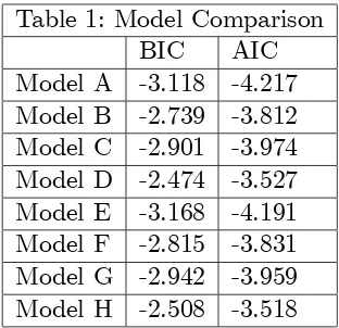
We use the posterior expectation of the Bayesian information criterion (BIC) and Akaike’s information criterion (AIC) to compare models.
4
Empirical Results
4.1
Data
(lloyds), Rabobank (rabobank), Royal Bank of Scotland (rboscotland), UBS (ubs), and WestLB (westlb). For each bank, we consider three term rates: one-month, three-month and twelve-month.
With regards to the explanatory variables in (1) and (2), for Zt we use
the implied volatility of overall stock prices (VIX). Djt is a measure of
bank-speci…c credit risk and inclusion of the VIX controls for volatility in the market as a whole (e.g. Hakkio and Keeton, 2009). In the equations with the LIBOR-OIS spreads as dependent variables, we set Xt to be the
commonly-used Term Auction Facility (TAF) dummy variable (which equals one for auction dates) when the Fed was injecting liquidity into the markets. We include Xt only in the equations involving the USD.
Both LIBOR-OIS spread and CDS rate are measured in basis points, while VIX is a percentage. To have all the data of approximately the same magnitude, we divide both CDS and VIX data by 100 and demean all the variables. Excluding common holidays and weekends,5 we have 727
observa-tions for each variable.
4.2
Model Comparison
In addition to the very ‡exible unrestricted model described in Section 2, we estimate several restricted models which reduce the number of latent liquidity factors and/or remove the Markov switching part of the model. Altogether, we estimated eight models:
Model A (the Full Model): One latent credit risk factor, three latent liquidity risk factors in USD, GBP and EUR, respectively.
Model B: One latent credit risk factor, one common latent liquidity risk factor in USD and GBP, one unique latent liquidity risk factor in EUR.
Model C: One latent credit risk factor, one unique latent liquidity risk factor in USD, one common latent liquidity risk factor in GBP and EUR.
Model D: One latent credit risk factor, one common latent liquidity risk factor in USD, GBP and EUR.
Model E: Same as Model A but without Markov switching.
Model F: Same as Model B but without Markov switching.
Model G: Same as Model C but without Markov switching.
Model H: Same as Model D but without Markov switching.
Before presenting empirical results relating to …nancially-relevant features of interest, it is important to present statistical information on which models are supported by the data. Table 1 reports AIC and BIC for these eight models. The …rst point that stands out is that neither of the information criteria vary by a large amount across models. If we were to do a Bayesian model averaging exercise using the information criteria to construct model weights, then all of the models would receive appreciable probability. Sec-ondly, Models A (the full unrestricted model) and E (which is the same as Model A except removes the Markov switching component of the model) are the two models which perform best according to both information criteria. AIC chooses the Model A as being best whereas the more parsimonious BIC chooses Model E.
Table 1: Model Comparison BIC AIC Model A -3.118 -4.217 Model B -2.739 -3.812 Model C -2.901 -3.974 Model D -2.474 -3.527 Model E -3.168 -4.191 Model F -2.815 -3.831 Model G -2.942 -3.959 Model H -2.508 -3.518
4.3
Financial Features of Interest
4.3.1 The Factors
In light of the …ndings of the preceding sub-section, in our discussion of …nancial features of interest, we will restrict our attention to the Full Model (Model A) and the Best Model (Model E) selected by BIC.
There are many …nancially-interesting features of interest in our modelling framework. In addition to the parameters in the model, we can present the latent factors, Lkt and Ct, which shed light on liquidity and credit risk. For
the Full Model, we can also present the probabilities of our four states (i.e.
f(GL; GC);(BL; GC);(GL; BC);(BL; BC)g) relating to the Markov switching
aspect of the model
Furthermore, to investigate the relative roles of credit and liquidity risks in the …nancial crisis, we also present a variance decomposition based on the LIBOR-OIS equations. As explained in McAndrews et al (2008), credit and liquidity risks might be correlated. Additionally, the latent risk factors might not be orthogonal to Xk. The existence of possibly correlated components
renders variance decomposition a less straightforward exercise. From (1), we have the following:
var(Sijkt) = Sijk
2
var(Lkt) + Sij
2
var(Ct) +
0
ik 2
var(Xt) +var "Sijkt(5)
+2 Sijk Sijcov(Lkt; Ct) + 2 Sijk ijcov(Lkt; Xt) + 2 Sij
0
ikcov(Ct; Xt):
decomposition will allow us to see the the relevant importance of the di¤erent terms on the right hand side of (1).
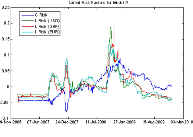
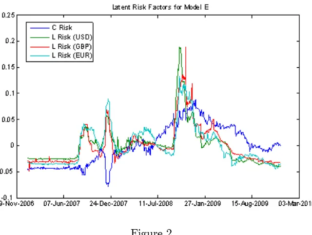
The posterior mean of the latent credit and liquidity risks are presented in Figure 1 (for the Full Model) and Figure 2 (for the Best Model).6 Figure
1 and Figure 2 exhibit almost identical patterns, indicating that the addition of Markov switching states adds little to our understanding of credit and liquidity risk. The three liquidity risk factors tend to move together (although there are some important di¤erences between them which we will note below) in a manner that is quite di¤erent from the credit risk factor.
First let us consider credit risk. This tended to grow gradually from August 2007 to a peak in December 2008, before gradually decreasing. By the end of 2009, credit risk was still at a level higher than in August 2007, the time when the …nancial turmoil …rst emerged. However, it is interesting to note the two clear dips in credit risk before December 2008. The …rst happened in December 2007. This was around the time when many banks were forced to take additional large write downs. Furthermore, the Fed’s term auction facility (TAF) …rst opened on December 17, 2007 (although the dip in Figures 1 and 2 began well before December 17). It seems that immediate response in the market to these events was that the perceived credit risk dropped, though this drop only lasted for the month of December 2007 and by January 2008 credit risk returned to where it had been before the dip began. The second smaller drop (or a plateau in the gradual increase) in credit risk happened in the summer of 2008. However, by late summer of 2008, the gradual increase in credit risk resumed (even before Lehman Brothers …nally went bankrupt in September 2008 and AIG disclosed that it faced serious liquidity shortage). It worth mentioning that credit risk remained at a high level throughout 2009, only slightly lower than its December 2008 peak. But it is worth stressing that the movements in the latent credit risk tend to be gradual and there is no huge spike in credit risk in autumn 2008.
In contrast to the credit risk, liquidity risks rose and dropped more abruptly. Figures 1 and 2 show that there were three major upsurges in liquidity risk, with by far the largest being at the time when the …nancial crisis was at its worst (i.e. in autumn 2008). The other two peaks in liquidity risk occurs in August 2007 and December 2007. August 2007 is often cited as the beginning of the …nancial crisis when Northern Rock’s problems became clear. Also in August, central banks implemented a wide range of
dented liquidity easing approaches. For instance, European Central Bank (ECB) injected 95 billion Euros in overnight credit and the Fed injected $24 billion. Our methodology is …nding all liquidity risks to have dropped after an August 2007 peak, although this drop was much more rapid in the USD than the EUR market. The second peak, in early to mid-December 2007 is just before the time that the Fed’s term auction facility, TAF, began. It …rst opened on December 17, 2007 and our methodology is …nding liquidity risk to have fallen shortly after this.
During all of these upsurges, liquidity risks in the three di¤erent currencies behaved broadly similarly to one another. However, there are many minor di¤erences in their behavior (which presumably accounts for why models with fewer than three liquidity factors performed poorly in Table 1). One notable di¤erence is that the EUR liquidity risk exhibited a fourth upsurge in May and June 2008 which does not appear in the USD and GBP liquidity risks. Furthermore, as noted above, after the August 2007 increase in liquidity risk (common to all currencies), liquidity risk remained high in the EUR market well after it declined in the other currencies.
Another interesting di¤erence between currencies can be noted at the time that the credit crunch was at its worst. In October 2008, when all the three liquidity risks skyrocketed, liquidity risk in USD led those of the other currencies (and especially the GBP). Furthermore, the USD liquidity risk reached a higher level than the EUR liquidity risk. Interestingly, after reaching the peak, liquidity risks in USD and EUR dropped much more rapidly than those in the GBP currency market.
Figure 2
4.3.2 The Markov Switching States
Table 1 and the similarity of results in Figures 1 and 2 suggest that Markov switching is not an empirically vital aspect of our model. It seems that al-lowing for the gradual evolution of factors, as state equations such as (3) and (4) would allow for (even if we removed the Markov switching state variable), is adequate to capture the main empirical features of the data. Nevertheless, our Full Model which includes the Markov switching does receive apprecia-ble support in Taapprecia-ble 1, so it is worthwhile to brie‡y present empirical results relating to this aspect of the model.
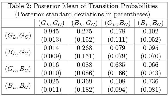
Table 2 presents information about the posterior of the matrix of tran-sition probabilities. We …nd that 90% of the time the model is either in the (GL; GC) or (BL; BC) state. This accounts for why the probabilities for
[image:15.612.150.470.142.383.2]estimate tells us the probability of remaining there is 74%).
Table 2: Posterior Mean of Transition Probabilities (Posterior standard deviations in parentheses)
(GL; GC) (BL; GC) (GL; BC) (BL; BC)
(GL; GC)
0:945 (0:013)
0:275 (0:152)
0:178 (0:111)
0:102 (0:052)
(BL; GC)
0:014 (0:009)
0:268 (0:151)
0:079 (0:079)
0:095 (0:070)
(GL; BC)
0:016 (0:010)
0:088 (0:086)
0:635 (0:166)
0:066 (0:043)
(BL; BC)
0:025 (0:011)
0:369 (0:182)
0:108 (0:094)
0:736 (0:081)
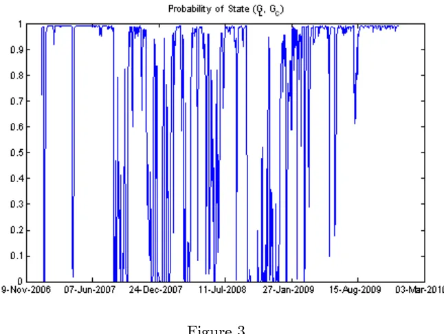
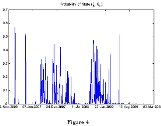
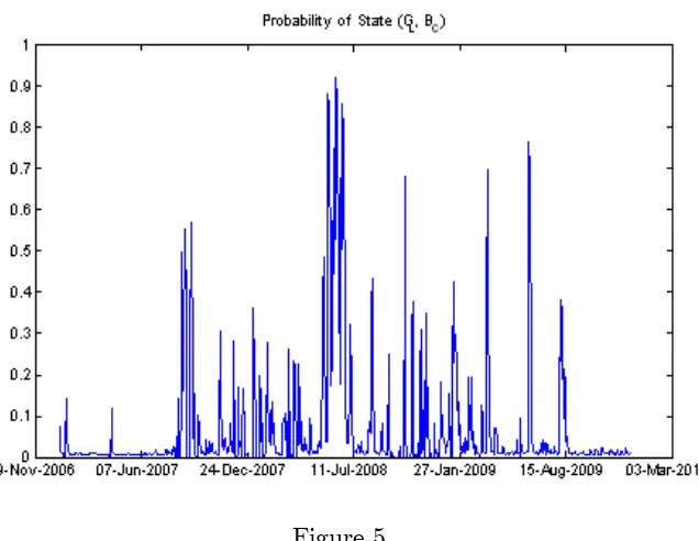
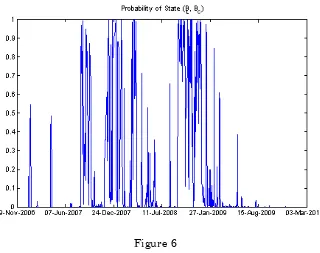
Figures 3 through 6 plot posterior means of the states themselves for the four states. Figures 3 and 6 are of most interest since, as just discussed, the states plotted in Figures 4 and 5 (i.e. (BL; GC) and (GL; BC)) rarely occur
in our data set. Given this fact, Figures 3 and 6 can be seen (approximately) to be mirror images of each other. Our main …ndings are that, at the heart of the credit crunch (from mid-September through mid-November 2008), the bad liquidity and bad credit state holds (with a few exceptions). The other periods when the bad liquidity and credit state often has high probability are similar to periods discussed previously and associated with the liquidity risk upsurges noted in Figures 1 and 2. These are late August through mid-September, 2007 and December 2007.
Figure 6
4.3.3 Variance Decompositions
Our results thus far suggest that both liquidity and credit risk played a role in the …nancial crisis, although perhaps the former played a more important role than the latter. The variance decomposition of (5) can be used to formalize these …ndings. Noting that this decomposition relates tovar(Sijkt), it follows
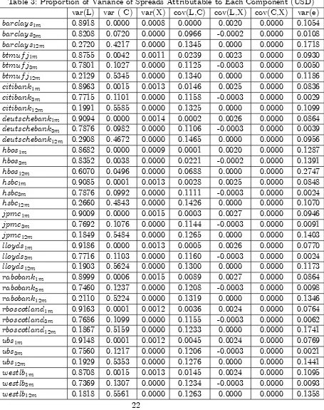
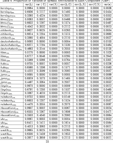
that we will have a variance decomposition for each bank, term and currency (i.e. each i; j and k). These are presented in Tables 3, 4 and 5 for the Full Model. Results using the Best Model are similar and will not reported here for the sake of brevity.
[image:20.612.150.470.138.391.2]LIBOR-OIS spreads, we have strong evidence that liquidity risk has been the major driver. For the GBP, the proportion of the variability in one month spreads attributable to the liquidity risk factor is typically very near to one (e.g. numbers like 0.99 or 0.98 are common) and never less than 0.80. For the USD and EUR markets the role of liquidity risk, although still high, is somewhat lower (e.g. numbers like 0.83 and 0.85 are common).
At the three month term, a similar pattern holds but the role of liquidity risk is somewhat less than at the one month term. But there are important di¤erences across currencies. That is, in the USD markets, liquidity risk typically accounts for 75 or 80% of the variability in spreads. But in the GBP market these numbers tend to be around 65% and in the EUR markets even lower than this.
At the 12 month term, however, a di¤erent picture emerges. At this longer term, credit risk assumes a much more important role. Although there is some variation across currencies and over banks, we are tending to …nd credit risk to account for about 50% of the variability in spreads in the USD markets (results for the GBP are slightly lower and EUR slightly higher than this). Liquidity risk is still important, tending to account for 20 or 30% of the variability in spreads in the USD markets (with results for the GBP being slightly higher and EUR slightly lower than this). However, credit risk is clearly the more important factor at this longer term in the vast majority of cases.
The role of the covariance between the liquidity and credit risk factors tends to be fairly small, accounting for typically around 10% of the variability in spreads. The other covariance terms in the variance decomposition play a negligible role. The dummy explanatory variable containing the TAF auction dates also explains little of the variation in spreads.
Note that the main dependent variable in our study isSijkt, as opposed to
most of the related literature which works withSt. The preceding discussion
risk factor for HBOS, at all terms and in all currencies, consistently is very low. Especially at longer horizons they are much lower than the other banks in the sample.
4.4
Robustness to Modelling Assumptions
In this paper, we have presented results using a very ‡exible model and compared the full model to several restricted versions of it. We have used a proper, but relatively noninformative prior and a sensible identi…cation scheme. We have investigated other modelling assumptions and have found our results to be very robust. Since these investigations do not substan-tively alter the empirical conclusions of this paper (and for the sake of brevity), we do not present these additional empirical results here. In-stead they are included in the Technical Appendix to this paper available at http://personal.strath.ac.uk/gary.koop/.
Table 3: Proportion of Variance of Spreads Attributable to Each Component (USD) var(L) var ( C) var(X) cov(L,C) cov(L,X) cov(C,X) var(e)
barclays1m 0.8918 0.0000 0.0008 0.0000 0.0020 0.0000 0.1054
barclays3m 0.8208 0.0720 0.0000 0.0966 -0.0002 0.0000 0.0108
barclays12m 0.2720 0.4217 0.0000 0.1345 0.0000 0.0000 0.1718
btmuf j1m 0.8755 0.0042 0.0011 0.0239 0.0023 0.0000 0.0930
btmuf j3m 0.7801 0.1027 0.0000 0.1125 -0.0003 0.0000 0.0050
btmuf j12m 0.2129 0.5345 0.0000 0.1340 0.0000 0.0000 0.1186
citibank1m 0.8963 0.0015 0.0013 0.0146 0.0025 0.0000 0.0836
citibank3m 0.7715 0.1101 0.0000 0.1158 -0.0003 0.0000 0.0029
citibank12m 0.1991 0.5585 0.0000 0.1325 0.0000 0.0000 0.1099
deutschebank1m 0.9094 0.0000 0.0014 0.0002 0.0026 0.0000 0.0864
deutschebank3m 0.7876 0.0982 0.0000 0.1106 -0.0003 0.0000 0.0039
deutschebank12m 0.2908 0.4672 0.0000 0.1465 0.0000 0.0000 0.0956
hbos1m 0.8682 0.0000 0.0009 0.0001 0.0020 0.0000 0.1287
hbos3m 0.8352 0.0038 0.0000 0.0221 -0.0002 0.0000 0.1391
hbos12m 0.6070 0.0496 0.0000 0.0688 0.0000 0.0000 0.2747
hsbc1m 0.9085 0.0001 0.0013 0.0028 0.0025 0.0000 0.0848
hsbc3m 0.7876 0.0992 0.0000 0.1111 -0.0003 0.0000 0.0024
hsbc12m 0.2660 0.4843 0.0000 0.1426 0.0000 0.0000 0.1070
jpmc1m 0.9009 0.0000 0.0015 0.0003 0.0027 0.0000 0.0946
jpmc3m 0.7692 0.1076 0.0000 0.1144 -0.0003 0.0000 0.0091
jpmc12m 0.1849 0.5484 0.0000 0.1265 0.0000 0.0000 0.1403
lloyds1m 0.9186 0.0000 0.0013 0.0005 0.0026 0.0000 0.0770
lloyds3m 0.7716 0.1103 0.0000 0.1160 -0.0003 0.0000 0.0024
lloyds12m 0.1903 0.5624 0.0000 0.1300 0.0000 0.0000 0.1173
rabobank1m 0.8999 0.0006 0.0015 0.0089 0.0027 0.0000 0.0864
rabobank3m 0.7460 0.1237 0.0000 0.1208 -0.0003 0.0000 0.0098
rabobank12m 0.2110 0.5224 0.0000 0.1319 0.0000 0.0000 0.1346
rboscotland1m 0.9163 0.0001 0.0012 0.0036 0.0024 0.0000 0.0764
rboscotland3m 0.7686 0.1099 0.0000 0.1155 -0.0003 0.0000 0.0062
rboscotland12m 0.1867 0.5159 0.0000 0.1233 0.0000 0.0000 0.1741
ubs1m 0.9148 0.0001 0.0012 0.0045 0.0024 0.0000 0.0769
ubs3m 0.7560 0.1217 0.0000 0.1206 -0.0003 0.0000 0.0021
ubs12m 0.1929 0.5353 0.0000 0.1276 0.0000 0.0000 0.1441
westlb1m 0.8708 0.0015 0.0013 0.0145 0.0024 0.0000 0.1095
westlb3m 0.7369 0.1307 0.0000 0.1234 -0.0003 0.0000 0.0093
Table 4: Proportion of Variance of Spreads Attributable to Each Component (GBP) var(L) var ( C) var(X) cov(L,C) cov(L,X) cov(C,X) var(e)
barclays1m 0.9964 0.0000 0.0000 0.0000 0.0000 0.0000 0.0036
barclays3m 0.6936 0.1117 0.0000 0.1493 0.0000 0.0000 0.0454
barclays12m 0.3393 0.4224 0.0000 0.2031 0.0000 0.0000 0.0352
btmuf j1m 0.9363 0.0081 0.0000 0.0466 0.0000 0.0000 0.0091
btmuf j3m 0.6632 0.1297 0.0000 0.1574 0.0000 0.0000 0.0497
btmuf j12m 0.4042 0.3832 0.0000 0.2112 0.0000 0.0000 0.0013
citibank1m 0.9627 0.0025 0.0000 0.0263 0.0000 0.0000 0.0084
citibank3m 0.6614 0.1204 0.0000 0.1515 0.0000 0.0000 0.0668
citibank12m 0.3860 0.4004 0.0000 0.2110 0.0000 0.0000 0.0027
deutschebank1m 0.9893 0.0000 0.0000 0.0004 0.0000 0.0000 0.0103
deutschebank3m 0.6811 0.1194 0.0000 0.1530 0.0000 0.0000 0.0464
deutschebank12m 0.4663 0.3144 0.0000 0.2055 0.0000 0.0000 0.0138
hbos1m 0.8170 0.0000 0.0000 0.0003 0.0000 0.0000 0.1828
hbos3m 0.6717 0.0046 0.0000 0.0295 0.0000 0.0000 0.2943
hbos12m 0.5569 0.0366 0.0000 0.0764 0.0000 0.0000 0.3301
hsbc1m 0.9705 0.0001 0.0000 0.0057 0.0000 0.0000 0.0236
hsbc3m 0.6560 0.1306 0.0000 0.1571 0.0000 0.0000 0.0563
hsbc12m 0.4222 0.3599 0.0000 0.2092 0.0000 0.0000 0.0087
jpmc1m 0.9895 0.0000 0.0000 0.0005 0.0000 0.0000 0.0099
jpmc3m 0.6919 0.1078 0.0000 0.1465 0.0000 0.0000 0.0538
jpmc12m 0.4497 0.3364 0.0000 0.2087 0.0000 0.0000 0.0052
lloyds1m 0.9978 0.0000 0.0000 0.0009 0.0000 0.0000 0.0012
lloyds3m 0.6791 0.1208 0.0000 0.1537 0.0000 0.0000 0.0465
lloyds12m 0.3867 0.4010 0.0000 0.2113 0.0000 0.0000 0.0010
rabobank1m 0.9702 0.0008 0.0000 0.0149 0.0000 0.0000 0.0141
rabobank3m 0.6683 0.1207 0.0000 0.1524 0.0000 0.0000 0.0587
rabobank12m 0.4470 0.3355 0.0000 0.2078 0.0000 0.0000 0.0097
rboscotland1m 0.9907 0.0002 0.0000 0.0067 0.0000 0.0000 0.0024
rboscotland3m 0.6555 0.1367 0.0000 0.1606 0.0000 0.0000 0.0471
rboscotland12m 0.3503 0.4340 0.0000 0.2093 0.0000 0.0000 0.0064
ubs1m 0.9861 0.0003 0.0000 0.0084 0.0000 0.0000 0.0052
ubs3m 0.6411 0.1411 0.0000 0.1614 0.0000 0.0000 0.0564
ubs12m 0.4013 0.3863 0.0000 0.2113 0.0000 0.0000 0.0011
westlb1m 0.9665 0.0025 0.0000 0.0265 0.0000 0.0000 0.0045
westlb3m 0.6500 0.1459 0.0000 0.1653 0.0000 0.0000 0.0388
Table 5: Proportion of Variance of Spreads Attributable to Each Component (EUR) var(L) var ( C) var(X) cov(L,C) cov(L,X) cov(C,X) var(e)
barclays1m 0.8953 0.0000 0.0000 0.0000 0.0000 0.0000 0.1047
barclays3m 0.6521 0.1986 0.0000 0.1391 0.0000 0.0000 0.0101
barclays12m 0.2183 0.5940 0.0000 0.1392 0.0000 0.0000 0.0485
btmuf j1m 0.8509 0.0154 0.0000 0.0441 0.0000 0.0000 0.0896
btmuf j3m 0.6115 0.2391 0.0000 0.1478 0.0000 0.0000 0.0015
btmuf j12m 0.2308 0.5804 0.0000 0.1415 0.0000 0.0000 0.0474
citibank1m 0.8573 0.0045 0.0000 0.0240 0.0000 0.0000 0.1142
citibank3m 0.6327 0.2208 0.0000 0.1445 0.0000 0.0000 0.0020
citibank12m 0.2288 0.5784 0.0000 0.1406 0.0000 0.0000 0.0522
deutschebank1m 0.8600 0.0000 0.0000 0.0004 0.0000 0.0000 0.1396
deutschebank3m 0.5914 0.2377 0.0000 0.1449 0.0000 0.0000 0.0260
deutschebank12m 0.2786 0.5370 0.0000 0.1495 0.0000 0.0000 0.0348
hbos1m 0.8276 0.0000 0.0000 0.0003 0.0000 0.0000 0.1721
hbos3m 0.7510 0.0077 0.0000 0.0290 0.0000 0.0000 0.2123
hbos12m 0.5575 0.0610 0.0000 0.0711 0.0000 0.0000 0.3104
hsbc1m 0.8616 0.0003 0.0000 0.0051 0.0000 0.0000 0.1330
hsbc3m 0.6458 0.2079 0.0000 0.1416 0.0000 0.0000 0.0047
hsbc12m 0.2908 0.5170 0.0000 0.1499 0.0000 0.0000 0.0423
jpmc1m 0.9018 0.0000 0.0000 0.0005 0.0000 0.0000 0.0977
jpmc3m 0.6562 0.2013 0.0000 0.1405 0.0000 0.0000 0.0020
jpmc12m 0.2787 0.5280 0.0000 0.1483 0.0000 0.0000 0.0450
lloyds1m 0.8918 0.0000 0.0000 0.0009 0.0000 0.0000 0.1073
lloyds3m 0.6309 0.2220 0.0000 0.1447 0.0000 0.0000 0.0024
lloyds12m 0.2037 0.6015 0.0000 0.1353 0.0000 0.0000 0.0595
rabobank1m 0.8816 0.0015 0.0000 0.0137 0.0000 0.0000 0.1032
rabobank3m 0.6043 0.2301 0.0000 0.1442 0.0000 0.0000 0.0214
rabobank12m 0.2736 0.5323 0.0000 0.1475 0.0000 0.0000 0.0467
rboscotland1m 0.8773 0.0003 0.0000 0.0060 0.0000 0.0000 0.1164
rboscotland3m 0.6107 0.2350 0.0000 0.1465 0.0000 0.0000 0.0078
rboscotland12m 0.1847 0.6213 0.0000 0.1309 0.0000 0.0000 0.0630
ubs1m 0.8353 0.0005 0.0000 0.0078 0.0000 0.0000 0.1564
ubs3m 0.5832 0.2578 0.0000 0.1499 0.0000 0.0000 0.0091
ubs12m 0.2277 0.5860 0.0000 0.1412 0.0000 0.0000 0.0451
westlb1m 0.8539 0.0043 0.0000 0.0234 0.0000 0.0000 0.1184
westlb3m 0.5929 0.2518 0.0000 0.1494 0.0000 0.0000 0.0059
5
Conclusion
In this paper, we have motivated and developed a statistical model which uses a panel of LIBOR-OIS spreads and bank CDS rates to disentangle liq-uidity and credit risk. The panel dimensions of the spreads include variation across banks, currencies and terms. The existing literature almost always ignores these panel dimensions and simply works with one average LIBOR-OIS spread. From a statistical point of view, our empirical results show that there are bene…ts from exploiting these panel dimensions in terms of increasing our understanding of liquidity and credit risk.
References
Basel Committee on Banking Supervision, 2000, Sound practices for man-aging liquidity in banking organisations, consultative document available at http://www.bis.org/publ/bcbs69.pdf.
Basel Committee on Banking Supervision, 2001, The new Basel capital accord, consultative document available at http://www.bis.org/publ/bcbsca03.pdf.
Brunnermeier, M., 2009. Deciphering the liquidity and credit crunch 2007–2008. Journal of Economic Perspectives. 23, 77-100.
Campbell, J., Ammer, J., 1993. What moves the stock and bond markets? A variance decomposition for long-term asset returns. Journal of Finance. 48, 3-37.
Hakkio, C., Keeton, W., 2009. Financial stress: What is it, how can it be measured, and why does it matter? Federal Reserve Bank of Kansas City Economic Review. Third Quarter, 5-50.
Hui, C., Chang, T., Lo, C., 2010. Using interest rate derivative prices to estimate LIBOR-OIS spread dynamics and systemic funding liquidity shock probabilities. Hong Kong Monetary Authority, working paper 04/2010.
Kim, C. and Nelson, C., 1999. State Space Models with Regime Switch-ing. MIT Press, Cambridge, MA.
McAndrews, J., Sarkar, A., Wang, Z., 2008. The e¤ect of the term auction facility on the London inter-bank o¤ered rate. Federal Reserve Bank of New York Sta¤ Report No. 335.
Michaud, F., Upper, C., 2008. What drives interest rates? Evidence from the Libor panel. BIS Quarterly Review, March, 47-58.
Sengupta, R., Tam Y., 2008. The LIBOR-OIS spread as a summary indicator. Monetary Trends, Federal Reserve Bank of St. Louis, Nov. 25.
Taylor, J., and Williams, J., 2008a. A black swan in the money market. Working Paper, Stanford University and the Federal Reserve Bank of San Francisco 2008-4.
Taylor, J., and Williams, J., 2008b. Further results on a black swan in the money market, Stanford Institute for Economic Policy Research Working Paper 07-046.
Thornton, D., 2009. What the Libor-OIS spread says, Economic Syn-opses, Federal Reserve Bank of St. Louis.