Computer Methods in Biomechanics and Biomedical Engineering Vol. 00, No. 00, November 2013, 1–24
Original Article
A numerical investigation of flow around octopus-like arms: near-wake vortex patterns and force development
A. Kazakidia, V. Vavourakisa†, D.P. Tsakirisa‡ and J.A. Ekaterinarisb,c
aInstitute of Computer Science, Foundation for Research & Technology - Hellas, Heraklion 70013, Greece;bInstitute of Applied & Computational Mathematics, Foundation for Research & Technology - Hellas, Heraklion 70013, Greece;cDepartment of
Mechanical and Aerospace Engineering, University of Patras, Patra 26500, Greece
(Received 00 Month 200x; final version received 00 Month 200x)
The fluid dynamics of cephalopods has so far received little attention in the literature, due to their complexity in structure and locomotion. The flow around octopuses, in particular, can be complicated due to their agile and dexterous arms, that frequently display some of the most diverse mechanisms of motion. Their recognized manipulative and locomotor skills could inspire the development of advanced robotic arms, able to operate in fluid environ-ments. Our primary aim was to study the hydrodynamic characteristics of such bio-inspired robotic models and to derive the hydrodynamic force coefficients as a concise description of the vortical flow effects. Utilizing computational fluid dynamic methods, the coefficients were computed on realistic morphologies of octopus-like arm models undergoing prescribed solid-body movements; such motions occur in nature for short durations in time, e.g. during reaching movements and exploratory behaviors. Numerical simulations were performed on translating, impulsively rotating, and maneuvering arms, around which the flow field struc-tures were investigated. The results reveal in detail the generation of complex vortical flow structures around the moving arms. Hydrodynamic forces acting on a translating arm depend on the angle of incidence; forces generated during impulsive rotations of the arms are inde-pendent of their exact morphology and the angle of rotation; periodic motions based on a slow recovery and a fast power stroke are able to produce considerable propulsive thrust, even leading to a maximum displacement of 0.39 arm-lengths per period of a self-propelling arm, while harmonic motions are not. Parts of these results have been employed in bio-inspired models of underwater robotic mechanisms. This investigation may further assist elucidating the hydrodynamics underlying aspects of octopus locomotion.
Keywords:computational fluid dynamics; hydrodynamics; biologically-inspired robots; biomimetics; aquatic locomotion; octopus
1. Introduction
Underwater robotic systems are increasingly being used for demanding real-world applications (e.g., search-and-rescue operations, industrial inspections, or shallow-and deep-water marine explorations; Yuh 2000), that point to an intensifying need for higher efficiency, maneuverability and controllability. Inspired by marine ani-mals with outstanding manipulative and locomotor skills—like the octopus—, un-derwater robot designs can employ dexterous robotic manipulators to improve their application scope. Current robotic models commonly simplify the effects of flow
†Present address: Centre for Medical Image Computing, University College London, WC1E 6BT, UK ‡Corresponding author. Email: [email protected]
ISSN: 1741-5977 print/ISSN 1741-5985 online c
2013 Taylor & Francis
(a) (b) (c) (d) (e) (f)
(g) (h) (i)
Figure 1. (a-f) Octopus reaching movement involving elongation and rotation of a single arm: a large part of the arm is stiffened and held almost straight during the motion (100ms lapse between frames; video sequence by Hanassy S, Botvinnik A, Flash T, Hochner B, unpublished results; personal communication). (g-i) Bi-pedal walking followed by head-up swimming during an exploratory behavior at which the octopus translates an extended arm towards a moving target: a portion of the arm is relatively straight and stiffened, while positioned at an angle with the direction of movement (Kazakidi et al. 2012b).
and, hence, the acting hydrodynamic forces (Ekeberg 1993; Ijspeert 2001; Yeku-tieli et al. 2005; Sfakiotakis and Tsakiris 2007). In fact, it has been pointed out that variations in the hydrodynamic forces may strongly affect the behavior and control of robotic models in a non-trivial manner, even leading to novel propulsion modal-ities (Zhu et al. 2002; Thomas et al. 2005; Boyer et al. 2008; Krieg and Mohseni 2010). A detailed characterization of the flow field around aquatic animal bodies and understanding of how the fluid dynamic forces are generated could, therefore, provide valuable information for the design and accuracy of robotic models; infor-mation that only recently started to emerge for the octopus and octopus-inspired robotic arm manipulators (Kang et al. 2011; Sfakiotakis et al. 2012; Kazakidi et al. 2012a,b), but is still largely unclear, and is the subject of the current paper. Within our group’s ongoing efforts to develop robotic artefacts inspired by the octopus, the purpose of this study is to derive hydrodynamic force characteristics applicable to their dynamical models.
The octopus arms are highly agile and dexterous, despite their lack of skeletal support, and, therefore, of a particular interest to the design of robotic manipula-tors (octopus arms are muscular hydrostats according to Kier and Smith (1985); other examples of muscular hydrostats include squid tentacles, elephant trunks, and mammalian tongues). They can perform a variety of highly complex move-ments, like reaching and fetching, by shortening, elongating, bending, and twisting the arm muscles (Sumbre et al. 2001; Yekutieli et al. 2005; Huffard 2006). Oc-topuses exhibit unique cognitive skills and show a predilection of arm usage for executing specific tasks (Zullo and Hochner 2011; Gutnick et al. 2011). They may swim or crawl along the seabed, use jet propulsion during burst swimming and exert large forces by varying their arm stiffness. Commonly, reaching movements are achieved by bend propagation along the arm, during which a large portion of the arm is stiffened and held straight (Yekutieli et al. 2005). In addition, reach-ing motions may often involve rotation of the arm around its base, as is shown in figures 1a-f. In these figures, the arm appears to be rigidly stiffened and rotate in a more or less planar configuration. During the exploratory behavior of figures 1g-i, the octopus translates a rigidly extended arm towards a moving target. Such solid-body-like motions do occur in nature, even though only for short durations in time (see Section 4.1 for further discussion on these figures).
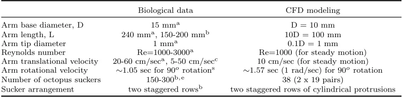
[image:2.595.90.470.47.188.2]Table 1. From biological organisms (Octopus vulgarisandOctopus bimaculoides) to Computational Fluid Dynamic (CFD) modeling (D is the arm base diameter).
Biological data CFD modeling
Arm base diameter, D 15 mma D = 10 mm
Arm length, L 240 mma, 150-200 mmb 10D = 100 mm
Arm tip diameter 1 mma 0.1D = 1 mm
Reynolds number Re=1000-3000a Re=1000 (for steady motion) Arm translational velocity 20-60 cm/seca, 5-50 cm/secc 10 cm/sec (for steady motion) Arm rotational velocity ∼1.05 sec for 90o rotations ∼1.57 sec (1 rad/sec) for 90o rotation
Number of octopus suckers 150-300b,e 38 (2 x 19 pairs)
Sucker arrangement two staggered rowsb two staggered rows of cylindrical protrusions aYekutieli et al. (2005).bGrasso (2008).cGutfreund et al. (1996).
dEstimation from video sequence of figure 1a-f.eIncluding those<1 mm in diameter.
organisms differ from their aerial counterparts in that the medium (water) in which they move has a much higher density than air, and is always incompressible. For animals with a body density comparable to that of water, gravity is nearly balanced out and the animal can remain suspended at a stationary depth, with little or no energy consumption (neutral buoyancy). Nevertheless, many marine organisms— including species of cephalopods—are slightly denser than seawater and sinking is avoided by regulating their buoyancy; for example, by swimming continuously or hovering actively, or by using other buoyancy mechanisms (swimbladders, vacuum systems, body fluids, etc.) (Alexander 1990; Webber et al. 2000). In doing so, they may expend a considerable amount of metabolic energy to generate hydrodynamic lift (buoyancy augmentation). For swimming at a steady speed, marine animals must produce enough directional thrust to balance vertical and lateral forces and overcome the induced hydrodynamic drag (Sfakiotakis et al. 1999; Lauder and Drucker 2002; Borazjani and Sotiropoulos 2008).
There is accumulating evidence, emerging primarily from studies of fish swim-ming (but also of bird flight), that some fish and other marine animals (as well as birds) have developed control mechanisms to exploit perturbations and unsteady flow features (e.g., vortices and vortex sheets), considerably reducing, as a result, the cost of locomotion and remarkably increasing their swimming (or flying) perfor-mance (Lauder 2010). For example, common fish species, of the orderPerciformes, appear to shed vortex rings in the wake of their body during locomotion, which, ac-cording to interspecies variations, could be paired or single, linked or discrete, and could reorient downstream or laterally with increasing speed to enhance or reduce, respectively, the hydrodynamic thrust (Lauder and Drucker 2002). Species of trout (of the order Salmoniformes) are able to further adapt their locomotion mecha-nism behind vortical structures that pre-exist in the flow stream (generated either artificially or as part of a schooling formation), by extracting energy from the vor-tices (K´arm´an gait) (Liao et al. 2003a,b) and reducing, therefore, their locomotion cost. Eels (of the order Anguilliformes), which have a more elongated and slender body shape than other fish, and have no separated caudal fin (caudal peduncle), generate jets of fluid directed only laterally, with no substantial downstream flow, when swimming steadily (Tytell and Lauder 2004; Tytell 2004). Furthermore, hy-dromedusan jellyfish (of the orderFilifera) generate, during jet propulsion, a single vortex per jet pulse, the size of which could be exploited by the animal via velar diameter changes to augment thrust and reduce locomotion costs (Dabiri et al. 2006). Finally, squid (of the order Teuthida) produce several vortical structures as a result of both jet propulsion and fin undulations; the latter showing a notable contribution to increased thrust and propulsive efficiency (Anderson and Demont 2000; Bartol et al. 2008).
the-oretical, or numerical methods, is not trivial, primarily due to their flexibility and agility. Furthermore, the estimation of the relationship between thrust and veloc-ity for use in robotic models can be ambiguous due to its dependence on multiple factors, such as the shape, the texture and the velocity of the arm. Hydrody-namic loads can also be naturally unsteady in time, due to fluctuations in the flow field, even if the arm is assumed to move at a constant velocity. A first at-tempt in developing mathematical models of octopus arm motions was made by Yekutieli et al. (2005); they performed force measurements on free-falling ampu-tated arms, reinforced with various gravitational loads in order to maintain a fixed shape, and demonstrated the strong influence of hydrodynamic forces on a planar arm-reaching movement. A theoretical approach could assume each of the eight arms as a right circular cone or tapered circular cylinder, due to the general shape of the arm, which is very long as compared to the lateral dimensions (the length to base-diameter ratio is estimated between 10 to 16, table 1) (Yekutieli et al. 2005; Grasso 2008). There are indeed numerous previous works on flows around circular and tapered cylinders which could provide some insight into this direction (e.g., Taylor 1952; Vall`es et al. 2002; Parnaudeau et al. 2007; Narasimhamurthy et al. 2009). However, about one third of the lateral sides of the arm is covered by suckers of various sizes and numbers (about 150-300, table 1; Grasso 2008), and although in general they are arranged in a structured way (in two staggered rows along the length of the arm), the suckers make the surface rough. It is particularly hard to suggest a theory of hydrodynamics for rough tapered geometries, since the generated loads would depend on the precise geometrical features of the roughness. In an approach to address these issues, we used computational fluid dynamics (CFD) simulations to study and quantify the flow over realistic morphologies of octopus-like arms undergoing prescribed solid-body movements. Examples of such type of movements are displayed in Figure 1, involving straight-arm tasks. Our aim was to derive hydrodynamic loads related to such movements that could be useful in robotic arm models and therefore, at first approximation, the octopus-like arms were assumed to be rigid in our numerical simulations. The study considers various distinct arm geometries and movements. It was divided into three parts: the hydrodynamic forces were calculated, firstly, for an arm positioned at various angles of incidence to a steady flow stream (this case corresponds to an arm mov-ing steadily at various inclined positions through a quiescent fluid); secondly, for impulsively rotating arm movements; and lastly, for periodic arm movements to examine thrust generation. For the second part, different arm morphologies were also compared. This study is a continuation of a preliminary work focusing on the effects of octopus-like suckers in straight-arm configurations and multi-segmented models (Kazakidi et al. 2012a). The results within the present work show how the hydrodynamic forces acting on moving octopus-like arms depend on the different types of prescribed motions, applicable to robotic arm models.
(a)
(b-i)
(b) (c)
(d) (c-i)
(b-i)
(c-i)
z y y
z
(d-i)
(d-i)
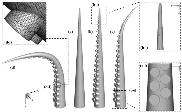
Figure 2. (a) Simplified octopus-like arm. (b-d) Octopus-like arm models, including pairs of cylindrical protrusions at the upstream face, positioned in a staggered configuration (oblique projection); (b) straight arm, (c) partially bent (convex) arm, (d) fully bent (concave) arm. Insets (b-i,c-i) show a close-up view of the three top- and bottom-most pairs of protrusions (frontal view). The inset (d-i) shows a detail of the surface mesh around an octopus sucker.
2. Methods
2.1 Octopus-like arm geometries
Four octopus-like arm geometries were considered in this study: a simplified arm (figure 2a); a straight arm with a staggered array of cylindrical protrusions repre-senting octopus suckers (figure 2b); an arm with a partial bend at the tip (convex configuration, figure 2c); and an arm with almost ninety degrees bend (concave configuration, figure 2d). The scope was not to replicate the exact anatomy of real octopus arms, as there are vast variations among octopus species (Huffard 2006), but to develop realistic arms, inspired primarily from the Octopus vulgaris and
Octopus bimaculoides (Table 1), for use in biomimetic robotic-arm models.
The straight arms were approximated as right circular conical frustums with a base diameter of D, tip diameter of 0.1D and length of 10D, which gave a taper ratio of approximately 11:1, defined as length/(base diameter – tip diameter), and an aspect ratio of approximately 18:1, defined as length/mean diameter. The rel-ative ratios of these dimensions are within the physiological scales of real octopus arm sizes (table 1; Yekutieli et al. 2005; Grasso 2008). The partially bent arm (convex configuration) was the same as the straight arm with protrusions near the base, but near the tip, approximately 33% of its length was made to follow a seg-ment of circle of 33.6D in radius (6 last pairs of protrusions, figure 2c). The fully bent arm (concave configuration) formed a smoothed ninety-degree bend with the longitudinal arm axis, near the middle.
[image:5.595.104.460.53.273.2]protrusions decreased by 0.01D, the first pair having a radius of 0.2D and the last 0.02D (insets in figure 2b-i, 2c-i). The first sucker had a height (in the negative x-direction) of 0.04D, while the height of each subsequent sucker decreased towards the arm tip by 0.01D. The center-to-center lateral separation of each sucker within a pair (in the y-direction) was equal to their respective diameter; that is, the inner lateral lips of all protrusions were aligned to the midline of the upstream face of the arm. The protrusions were staggered in the negative z-direction, with a center-to-center separation of 0.25D.
For all geometries, the computational domain was 46D long (in the x-direction), 31D wide (in the y-direction) and 20D high (in the z-direction). The upstream and lateral lips of the arm base were located 15D away from the upstream and lateral edges of the domain, respectively.
2.2 Governing equations and boundary conditions
The flow field induced by the arm motion in the water is governed by the incom-pressible Navier-Stokes equations (Batchelor 2000; Tritton 1988). A Newtonian fluid was considered (that is, its viscosity was assumed to be constant), described by the following formulation of the Navier-Stokes equations
∂u
∂t + (u· ∇)u=−
1
ρ∇p +ν∇
2u, (1)
∇ ·u=0, (2)
where u=[u, v, w] is the velocity vector, ρ is the fluid density, p is the pressure, and νis the kinematic viscosity. The flow is characterized by the Reynolds number (ReD), a non-dimensional parameter, defined as
ReD =
U D
ν , (3)
where U is the free stream velocity of the fluid, and D is the characteristic length (here, D is the base diameter of the octopus arm). The Reynolds number is a measure of the ratio of inertial forces (ρU2) to viscous forces (µU/D). At high Reynolds numbers, inertial forces dominate, whereas viscous forces prevail at very low Reynolds numbers. Octopus arm movements in seawater are performed with a Reynolds number of the order of 1000 (Gutfreund et al. 1996; Yekutieli et al. 2005), and therefore, inertial forces dominate (ReD >>1).
For the first part of the study, we considered an arm positioned at various angles of incidence to a steady flow stream, where ReD was taken equal to 1000 (based on
the base diameter) and the upstream, bottom and side faces of the computational domain were assigned as inflow boundary conditions, using a uniform inlet velocity profile. The top and downstream faces were considered as pressure-outlets, while the no-slip condition was applied on the arm surface.
2.3 Hydrodynamic forces
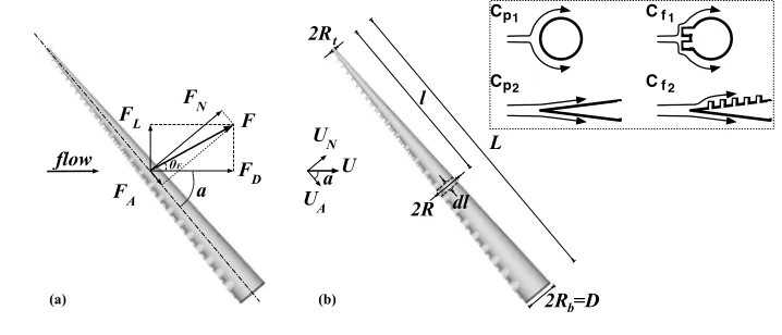
The total hydrodynamic force (F) acting on the arm, when positioned at an angle with respect to the direction of the oncoming flow (figure 3a), can be decomposed into components parallel and perpendicular to either the flow direction (drag, FD
U
L UN
2R =Db
UA
(b) a 2Rt
2R dl
l
Cp1
Cp2
Cf1
Cf2
F FN FL
a
flow F
D
FA
(a)
θF
Figure 3. Hydrodynamic loads acting on: (a) an octopus-like arm with protrusions and (b) an arm in-cluding an infinitesimal segment. In (a) the total hydrodynamic force (F) is decomposed into components parallel and perpendicular to either the flow direction (drag, FDand lift, FL, respectively) or the arm axis
(axial force, FAand normal force, FN, respectively). The inset illustrates decomposition into components
ascribable to pressure drag and skin friction drag, in the direction normal to the axis of the arm (top row, with coefficients Cp1, Cf1, respectively) and parallel to the axis of the arm (lower row, with coefficients Cp2, Cf2, respectively).
respectively). These are defined as
F =pFD2+FL2 =
p
FN2+FT2 (4)
FD =
1 2ρU
2C
DA, FL=
1 2ρU
2C
LA (5)
FN = 1
2ρU 2A (C
D sinα+CL cosα) (6)
FA=
1 2ρU
2A (C
D cosα−CLsinα) (7)
where CD and CL are the drag and lift coefficients, respectively, A is the reference
area, which here is taken as the projected frontal area of the straight arm, andαis the angle between the axis of the arm and the direction of the flow stream (angle of incidence).
When the arm includes a complicated array of protrusions representing octopus suckers, a more detailed description of the force development could be as follows (equivalent models for smooth and rough circular cylinders can be found in the literature, e.g., Taylor 1952): Consider an infinitesimal segment of diameter 2R and length dl on the arm (figure 3b), where R = Rt+ (Rb −Rt)l/L, and where
Rb, Rt are the base and tip radii of the arm, respectively, and l the position of
the segment along the arm of length L. Due to the roughness of the arm with the protrusions, the acting forces could be divided into components ascribable to pressure drag and skin friction drag. Therefore, the normal force acting on the arm segment, can be expressed as:
dFN =
1 2 ρU
2
N Cp1 dAp +
1 2 ρU
2 C
f1 sinα dAs (8)
where dAp= 2R dl is the projected area of the arm segment in the normal direction
and dAf = 2πR dl is the lateral surface area of the infinitesimal segment; UN is
[image:7.595.103.462.49.203.2]the arm, the above equation becomes:
FN = 1
2 ρU 2 (R
b+Rt) L(Cp1 sin2α+π Cf1 sinα) (9) Similarly, the axial force acting on the arm, can be expressed as:
FA=
1 2 πρU
2 [R2
b Cp2 cos2α+ (Rb+Rt) L Cf2 cosα] (10) whereπR2
b is the projected area of the segment in the axial direction. Cp2and Cf2
are the pressure drag and skin friction coefficients, respectively, in the direction parallel to the axis of the arm (inset of figure 3b, lower row).
In the previous description, the coefficient values could possibly be approximated by empirically known values (c.f., e.g., Taylor 1952; Potter and Wiggert 2002) for flow around circular cylinders and cones, respectively, and for the appropriate Reynolds number. Instead, for a steadily-moving straight octopus-like arm (see Section 3.1), we used the theoretical formulae of Eqs. 9, 10 to fit the CFD-obtained data, and find those values of the Cp1, Cp2 and Cf1, Cf2 coefficients that give the minimum root-mean-square (RMS) error with the CFD results. This approach is likely to give rise to a prediction model for the hydrodynamic forces generated also under other characteristics of the movement, e.g. for all intermediate angles of incidence, or for other aspect and taper ratios of the arm, and/or velocity values, which are useful for robotic arm models.
2.4 Computational tools
The ANSA (BETA CAE Systems S.A., http://www.beta-cae.gr) grid generation software package, which offers high accuracy and flexibility in generating user-specified element sizes, was used for the generation of hybrid-type meshes and body-fitted elements on the octopus-like arms. The bent arms were constructed with the use of a morphing technique available in ANSA.
The number of triangular elements used for the surface discretization of the cylin-drical protrusions ranged between 1054 and 3155, depending on their individual size, in diameter and height, and their location along the arm (cf. Section 2.1). Figure 2d-i illustrates an example of the triangular surface mesh used for one of the cylindrical protrusions, at approximately one quarter away from the arm base. The number of discretization points was found more than sufficient to numerically capture the geometrical details of the protrusions. Having ensured a well-defined surface mesh, a mesh consisting only from prismatic elements was constructed at the near wall region of each octopus arm. This prismatic volume mesh was extended outwards of the arm, up to a distance that encapsulates the boundary layer growth during the arm movement, enableing accurate capturing of viscous flow effects. The near wall region was composed of 10 layers of non-uniform thickness. The first ele-ment height was approximately 0.001D, where D is the arm base diameter, and a growth rate of 1.1 was used for the extra layers.
a first mesh of 0.63x10⁶ prismatic and 2.18x10⁶ unstructured tetrahedral elements was generated, in addition to a much finer one of a total of 24x106 elements. For the arm geometry with protrusions (figure 2b) three meshes were tested, one with 4.85x10⁶ unstructured tetrahedral elements, another with 6.46x10⁶ hybrid elements and a much finer one with 18.76x10⁶ tetrahedral elements, to capture vortex generation during periodic motions. The partially bent arm geometry (figure 2c) was solved with a mesh of 6.17x10⁶ hybrid elements, whereas the fully bent arm geometry (figure 2d) had a mesh including a total of 17.55x10⁶ elements.
Numerical simulations were carried out in Fluent (ANSYS, Canonsburg, PA), which implements the finite-volume method to solve the governing equations (Eqs. 1,2). Solution was obtained by utilizing the SIMPLE algorithm for pressure-velocity coupling, a second-order pressure discretization scheme and a second-order upwind discretization scheme for momentum. For the simulations of impulsively rotating and periodic arm movements, a moving mesh strategy was adopted, available in the flow solver. The computational mesh was made to follow exactly the arm for the entire duration of a movement, thus ensuring that the high-resolution volume mesh constructed around the arm was maintained at all instances. The meshes used for all cases examined in this paper are, therefore, considered to provide high resolution in the near-wall region, sufficient in capturing the viscous flow effects. The mesh quality and density in the near-wake field, guarantees good preservation of the generated vortex patterns, with little diffusion, thus ensuring accuracy and high fidelity in our computations.
2.5 Sensitivity analysis
Sensitivity analysis for the straight-arm geometry with cylindrical protrusions was carried out, by comparing results between a coarser and a finer mesh, as well as a double-sized arm. In the former case, an insignificant mesh dependency of about 0.6% for the drag coefficient was measured for the calculation of the flow at an angle of incidence 20o.
A validation study was also performed for viscous flow past a two-dimensional circular cylinder, to determine the mesh requirements for adequate vortex captur-ing, the accuracy in obtaining shedding frequency and unsteady loads, and the boundary conditions. The two-dimensional mesh for the validation study consisted of 65554 elements and the computational domain was 46 cylinder-diameters long (in the stream-wise direction) and 31 cylinder-diameters wide (in the cross-flow direction), which is identical to the xy-plane of the three-dimensional domain of the cases presented in this paerer, i.e. identical to a plane that is perpendicular to the longitudinal axis of the straight arm. The numerically evaluated lift and drag coefficients for a Reynolds number of 100 (which corresponds to the Reynolds number at the tip of the 3D octopus-like arm, from where flow separation primar-ily originates) were found in very close agreement with previous published results (Braza et al. 1986; Williamson and Brown 1998).
2.6 Data analysis
For visualization purposes, the results of the next section are presented using con-tours of vorticity magnitude, streamtraces of velocity colored by helicity, and iso-contours of theλ2 criterion (see definition below) showing the existence of vortices. The vorticity, ωv, is a vector quantity, representing the local rotation of a fluid
el-ement, and is defined as ωv = ∇ ×u. The helicity, H, is a measure of the angle
between the velocity and vorticity vectors, defined asH =R
u·(∇×u)d3r(Moffatt
and Tsinober 1992), and describes the topological linking and direction of rotation of vortex lines.
Wake vortex topology was determined with theλ2criterion, as proposed by Jeong and Hussain (1995), according to which, a vortex core is located at regions where the second eigenvalue λ2 of the S2+ Ω2 tensor is negative (S and Ω correspond, respectively, to the symmetric and antisymmetric parts of the velocity gradient). Vortex breakdown, according to Leibovich (1983), was identified by substantial perturbations in the structure of the generated vortices and transition to turbulence (Robinson et al. 1994; Ekaterinaris and Schifft 1993).
In our analysis, we also consider the integrated (unsteady) forces acting on dif-ferent arm morphologies, during various motions. Variation of these forces along a specific direction can yield a further insight into the different flow effects on each arm morphology and motion profile. Unless specified otherwise, force coefficients presented in this work were based on the projected frontal area of the straight arm (A = 5.5D2), using the reference values ofρ=1022 kg/m3 and U= 10 cm/sec.
3. Results
The results of our study are presented in the following order: near-wake vortex patterns and force development are analyzed, initially, for an octopus-like arm po-sitioned at angles spanning from zero to 90o, at intervals of 10o, with the oncoming
flow (figures 4-7; this case corresponds to an arm moving steadily at inclined posi-tions through a quiescent fluid); then, different geometries of the arms are consid-ered and examined under impulsively rotating movements (figures 8-9); and finally, the effects of periodic movements on thrust generation are presented (figures 10-13). In the first two cases, the arms moved in the ventral direction (protrusions facing the flow), reflecting realistic octopus arm reaching movements, during which the ventral face of the arm with the protrusions is exposed in order to reach an object (figure 1a-f).
3.1 Arm translation at constant speed
Figure 4 displays the arm of figure 2b positioned at various angles of incidence
α, with respect to the oncoming flow (from 10o to 90o, at intervals of 10o), and demonstrates how the characteristics of the flow and the pattern of the generated near-wake vortices depend on α. In general, although at small angles of incidence the flow was steady in the downstream region, at a critical angle (of about 50o) the flow exhibited natural fluctuations in time, above which full separation occurred and the flow remained unsteady.
For angles of incidence up to 30o (figures 4a-c), two counter-rotating vortices
Vorticity Magnitude
(h) (i)
70o 80o 90 o
8 6 4 2 (d)
Vorticity Magnitude
Vorticity Magnitude
40o 50o 60o
(e) (f)
8 6 4 2 (a)
Vorticity Magnitude
10o Flow 20o 30o
direction
(b) (c)
Vorticity Magnitude 8 6 4 2
(g)
Figure 4. Near-wake flow patterns for an octopus-like arm performing steady translational motions, at various angles of incidence. Contours of instantaneous vorticity magnitude, normalized by U/D, at five horizontal slices along the straight octopus-like arm with protrusions, overlaid by instantaneous velocity streamtraces (colored by helicity). Angles of incidenceα: (a) 10o, (b) 20o, (c) 30o, (d) 40o, (e) 50o, (f)
60o, (g) 70o, (h) 80o, (i) 90o(ν=µ/ρ= 10−6m2/sec, U= 10 cm/sec, Re
D=1000).
Helicity Helicity 40o Flow
direction
Flow direction
(a) (b)
50o
e)
50o
Flow direction
(c) (d)
d)
40o
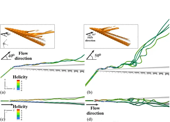
Figure 5. Details of instantaneous velocity streamtraces, colored by helicity, showing pairs of counter-rotating vortices on the lee side of steadily translating arms (only a part of the arm close to the tip is shown). (a-b) xz-plane. (c-d) yz-plane. (a,c)α=40o. (b,d)α=50o. The insets display iso-contours of λ
2, showing wake vortex topology (λ2= -50, Re=1000).
(figure 4b), they were strengthened and more extended; at α=30o (figure 4c), they further enlarged within a distinct separated region in the downstream area. In this range of angles, the vortices remained attached to the lee surface, for the entire length of the arm.
For mid-range values of the angle of incidence (40o-60o, figures 4d-f), the sepa-rated region downstream of the arm progressively enlarged with increasing α. At
[image:11.595.100.461.49.299.2] [image:11.595.135.424.364.572.2]Cd
tU/D
400 500 600 800 900 1000 0.1
700
(b)
0.101
0.099
Cd
tU/D
100 150 200 250
(a)
0.0845
0.084
Figure 6. Time evolution of the drag coefficient for (a)α=40o and (b)α=50o, respectively, for the last
stages of the simulations.
the base, an abrupt change in the structure of the vortices led to vortex breakdown. At α=50o (figure 4e), drastic variations in the vortices structure and detachment occurred even near the middle of the arm; whereas, atα=60o (figure 4f), the flow
detached almost near the tip. These features are more visible in figures 5a-d, which display close-up views of the instantaneous velocity streamtraces, colored by helic-ity, that strike the arm almost at the tip, forα=40o and 50o. According to figure 4, these streamtraces pass approximately through the centers of the vortices (vortex cores). They helped evaluate the angular displacement of the vortex cores with respect to the arm axis (z-axis of the computational domain), as well as estimate the location along the arm where vortex breakdown occurred, as presented in Table 2. Forα=50o, the vortex cores up to the detachment point were found at about 8o with the arm axis (in the xz-plane, figure 5b) and ±2o with the arm axis (in the
yz-plane, figure 5d); vortex breakdown occurred at a distance of about 66% of the arm length (measured from the base).
For large angles of incidence (70o-90o, figures 4g-i), flow perturbations were ex-tended further towards the tip of the arm, where complete detachment occurred. For these angles of incidence, an extended noncanonical structure of vortices was seen at the downstream region of the arm.
3.1.1 Hydrodynamic loads
The forces generated by the flow on the octopus-like arm were calculated by means of CFD methods for each of the cases described in the previous paragraphs. For α=10o-30o, the forces were steady in all directions. For α=40o, they reached a steady-state solution, although initially they were unsteady (figure 6a shows the time evolution of the drag coefficient). At the critical value of α=50o, the forces exhibited an oscillatory behavior (self-excited unsteadiness); however, the amplitudes of the oscillations were very small (figure 6b). The forces maintained their unsteady nature also for larger angles.
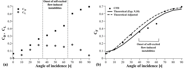
For each case of α, both the drag and lift coefficients showed similar temporal behavior. Across all cases, however, the coefficients differed substantially with α
(figure 7a). There was approximately a 15-fold difference between CD and CL, for
[image:12.595.133.422.50.149.2]α=0o and 90o. However, for most of the other angles, the coefficients had compa-rable values (1.5- to 2.8-fold difference), indicating the importance of both forces. Overall, the drag force coefficient increased with increasing angle of incidence. The
Table 2. Approximate vortex core angular displacements and vortex breakdown locations for angles of incidence
α=40o, 50o, and 60o, with respect to the arm axis (z
−axis of the computational domain), for steadily moving arms in thex−direction (figure 4).
α= 40o α= 50o α= 60o
Angular displacement with respect to the arm axis (in thexz-plane) 6.5o 8o 9o
Angular displacement with respect to the arm axis (in theyz-plane) ±1.7o
±2o
±2o
[image:12.595.82.476.675.724.2](
Onset of self-excited flow-induced
instabilities
(b)
Onset of self-excited flow-induced
instabilities
Angle of incidence [ ]o
Angle of incidence [ ]o
0.3
0 0.4 0.5 0.6 0.7
0.2
0.1
CL
C ,D 0.3
0 0.4 0.5 0.6 0.7
0.2
0.1
CF
0 10 20 30 40 50 60 70 80 90 0 10 20 30 40 50 60 70 80 90
CFD
Theoretical (Eqs. 9,10) Theoretical Adjusted C
C D L
Figure 7. Mean values of (a) the drag (CD) and lift (CF), and (b) the total force (CF) coefficients at ten
angles of incidence (0o-90o), for the steadily moving straight arm at inclined positions (the coefficients are
based on the projected frontal area of the arm).
lift coefficient, on the other hand, increased almost linearly withαfor angles up to 30o, dropped slightly for mid-range values of α, and then, after a small increase,
it decreased to almost zero. The reduction in the lift coefficient for angles between 40o and 60o is concomitant with the onset of natural fluctuations in the flow that
led to vortex breakdown. This also explains the delay in the growth of the drag co-efficient withα, at the same range of angles. It further explains the lowered values in the total force coefficient, CF, for the same angles of incidence, as displayed in
figure 7b.
In the same figure, the theoretical formulae suggested in Eqs. 9, 10 were used to find the best fit to the CFD-calculated values (solid line in figure 7b), as described in the Methods section (see Section 2). This model can fit sufficiently well with the CFD results for Cp1=0.27, Cp2=-0.39, Cf1=0.12, Cf2=-0.01 (the RMS error was 1.1x10⁻⁴; Table 3). However, the three lowered values of C
F between 40o and 60o,
at which self-excited flow-induced instabilities initiated, made the model to slightly underestimate the values of CF for the other angles of incidence. Recalculating the
RMS error after exclusion of these three lowered values (between 40o and 60o),
gave a better estimate for angles between 0o-30o and 70o-90o (dashed line in figure 7b), for which the RMS error was then 2.4x10⁻⁵ (C
[image:13.595.98.458.50.186.2]p1=0.07, Cp2=-0.15, Cf1=0.20, Cf2=0.03; table 3). With these models, the total force coefficient can, hence, be predicted also for all other intermediate angles of incidence, or for different aspect and taper ratios of the arm.
Table 3. Total force generated on a steadily translating octopus-like arm at various angles of incidence in a quies-cent fluid: value ofCF (column II) and direction of the
to-tal force vector (col. III), where tanθF=FL/FD=CL/CD.
CF was fitted by Eqs. 9, 10 (col. IV; RMS=1.1x10−
4
: Cp1=0.27, Cp2=-0.39,Cf1=0.12,Cf2=-0.01). Column V
gives the adjusted theoretical formulae after excluding three CF values at which flow-induced instabilities
initi-ated (RMS=2.4x10⁻⁵: C
p1=0.07, Cp2=-0.15, Cf1=0.20,
Cf2=0.03)
αo CCF D
F tanθF CF(Eqs.9,10) CFadjusted
[image:13.595.179.379.609.723.2]50o 30o
(a)
10o
50o 30o
(b)
10o
(c) 50o
30o 10o
50o 30o
(d)
10o
Vorticity Magnitude
8 6 4 2
ω ω
ω ω
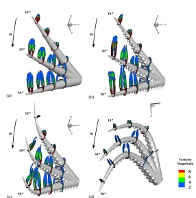
Figure 8. Impulsive rotations of octopus-like arms around the y-axis, at ω=1 rad/sec. Each subfigure depicts three distinct instances in time, at different angles of rotation. The near-wake flow is illustrated with contours of instantaneous vorticity magnitude, normalized by ωL/D, at four slices along (a) the simplified arm, (b) the straight arm with protrusions, (c) the partially bent arm (convex configuration), and (d) the fully bent arm (concave configuration), for 10o, 30o and 50o angles of rotation.
3.2 Impulsive rotation of the arm
The transient rotational movements of four distinct arm morphologies within an incompressible fluid, which is initially at rest, are shown in figure 8; all arms ro-tated around the y-axis with a constant angular speed of 1 rad/sec, which was estimated from the video sequence of figure 1a-f (Table 1). The arms moved in the ventral direction (protrusions facing the flow) from an initial position at zero angle of rotation between the longitudinal axis of the arm and the z-axis of the com-putational domain. Impulsive rotation of the simplified arm from rest produced a separated region on the lee side of the arm, which enlarged with increasing angle (figure 8a). Rotation of the straight arm with protrusions resulted in more extended and asymmetric counter-rotating vortices, generated within the separated region (figure 8b). Movement of the partially bent (convex) arm led to the diffusion of the vortices near and around the bent (figure 8c), with the development of a stronger shear layer that produced thinner and more elongated vortices. Finally, impulsively starting, rotational movement of the fully bent (concave) arm produced near-wake vortices that were substantially different from those of the other arm morphologies performing the same motion. The normalized magnitude of vorticity had lower val-ues at the corresponding slices along the arm, and the vortices were less extended (figure 8d).
To account for the different arm morphologies, the total force coefficients CF
[image:14.595.137.423.48.338.2]Angle of incidence [ ]o
0 10 20 30 40 50 60 70 80 90 0.3
0.4
0.2
C F
Average
Fully bent (concave) arm Partially bent (convex) arm Straight arm
Simplified arm
Figure 9. Total force coefficient during impulsive rotations of four arm morphologies around the y-axis, at 1 rad/sec, scaled with the ratio of total length to projected length of each arm morphology. Dashed line indicates the average curve.
35o-45o angle of rotation, then moderately increased up to about 70o, after which it faintly rose (up to 90o). In addition, the variation in the values of C
F with
increas-ing angle of rotation was quantitatively small, for each case. Hence, it could be postulated that CF is nearly independent of the angular position of the individual
arm. It is also apparent that the values of CF were almost independent of the exact
arm morphology, for all angular positions. It is, therefore, reasonable to calculate an average of the angular evolution of the total force coefficient, as representative for impulsively rotating arms (dashed line in figure 9), that could be applied to robotic models. This averaging can further be seen as a derived curve of CF for
this type of movement. For the values of the average curve of CF between 10o and
90o, the mean C
F was approximately 0.225.
3.3 Periodic motion of the arm
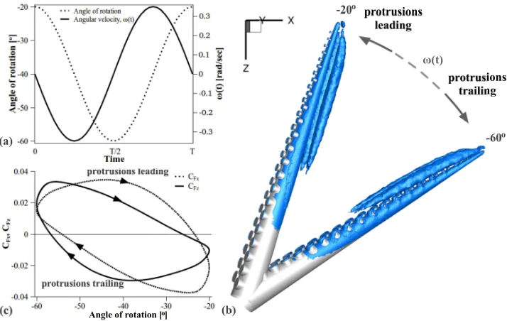
Inspired by the octopus arm swimming patterns (Huffard 2006), which in general involve movements of the arms in synchrony with a power (closing) and a recovery (opening) stroke of the arms (Kazakidi et al. 2012b; Sfakiotakis et al. 2012), we examined two different periodic profiles: a harmonic oscillation (figure 10a, solid line) and a “sculling” movement (figure 11, solid line). In both cases, the arm was prescribed to move periodically around the -40o angular position, in the xz-plane, with an angular span of ±20o. These values were rather arbitrary, but served as
a pattern of motion for a one-arm system, in which we wished to investigate the possible generation of forward thrust (in the positive z-direction). A third motion was achieved by allowing the arm to slide freely along the z-axis as a result of the propulsive force generated by the sculling motion (self-propelling arm).
1) A harmonic oscillatory motion was examined first, at which the straight arm with protrusions was made to rotate with a time-varying angular velocity ofω(t) =
−0.35 sin(t) rad/sec (figure 10a, solid line). For half of the period, the arm moved in the dorsal direction (from -20o to -60o) with the protrusions trailing and, for the other half, the arm moved from -60o to -20o in the ventral direction (with the
[image:15.595.154.404.51.239.2]protrusions leading
protrusions trailing
protrusions trailing protrusions
leading
-20o
-60o
(c) (b)
(a)
ω(t)
Angle of rotation [ ]o
Figure 10. Straight octopus-like arm performing harmonic oscillatory motion around the -40o angular
position (in the xz-plane). (a) Motion profile. (b) Instantaneous iso-contours of theλ2 criterion showing vortex topology for the two extreme angular positions (λ2= -5): movement in the ventral direction (protru-sions leading) is performed from -60oto -20o, while movement in the dorsal direction (protrusions trailing)
is from -20o to -60o. (c) C
F xand CF zforce coefficients.
stroke. For both extreme angular positions, the appearance of well-formed vortices was apparent (figure 10b displays instantaneous vortical structures at the end of the two strokes).
The CF x and CF z force coefficients are displayed in figure 10c, as a function of
the angle of rotation. Time-periodicity was achieved after about 1.5 periods. The results show that the force components varied with the angle of rotation and with the orientation of the oscillation (leading versus trailing faces): for CF z, the motion
produced positive thrust during most of the protrusions-leading stroke and negative thrust during most of the protrusions-trailing stroke, resulting in an effectively almost zero forward thrust in the positive z-direction (integral of the CF z curve
with respect to the angle of rotation for one complete period).
2) The second periodic motion was a “sculling” movement (Sfakiotakis et al. 2012), composed of a fast power and a slow recovery strokes. It involved a constant angular velocity ofωrecovery= 0.87 rad/sec for the recovery stroke, and a five-times
larger maximum velocity of ωpower = 4.36 rad/sec for the power stroke, at a ratio
between recovery-stroke duration and power-stroke duration of approximately 3.6. This sculling motion was prescribed in the CFD code by a polynomial expression forω(t) (solid line in figure 11), that was C2 continuous at all points and the area integral over the entire time period was zero. Like in the previous case, the arm rotated around the -40o angular position, in the xz-plane, with an angular span of ±20o. This motion profile was tested on both the simplified arm (see figures
12a,d) and the straight arm with protrusions (see figures 12b,e), in order to further examine the effects of protrusions on the generated forces and vortex evolution.
[image:16.595.101.458.48.274.2]even though they are captured at the end of the second period and beginning of the third period of the simulations, respectively. Regions of similar vortical structures are indicated with latin numerals, using the subscripts of p and r to mark the power and recovery strokes, respectively.
Concentrating first on the arm with protrusions and observing figures 12b and 12e together, it appears that vortical structures in regionsIp andIrwere remnants
of a previous transition between power and recovery strokes; flow structures in re-gions IIp andIIr were formed during the (slow) recovery stroke; and structures in
regions IIIp and IIIr were generated during the (fast) power stroke. Overall,
dur-ing the transition from the recovery to the early stages of the power stroke (until the maximum value ofωpowerwas reached), a concentrated region of separated flow
was generated on the protrusions-free side of the arm (figure 12b, region IIIp). In
the short duration of the power stroke, the arm moved at a very large angular veloc-ity with the protrusions-face leading the movement, resulting in large separation of the flow past the staggered protrusions (figure 12e, regionIIIr). At the end of the
power stroke and the transition to the recovery stroke, the arm decelerated heav-ily, resulting in the development of complex three-dimensional, counter-rotating vortical structures as flow separated in the opposite direction past the protrusions (figure 12e, regions Ir and IIr, and figure 12b, region Ip).
Comparing these regions of vortical structures with those obtained at the same instances in time for the smooth, simplified conical arm (figures 12a,d), it is clear that the protrusions have a notable impact on the fine details of the vortex evolu-tion around the sculling arm. For example, a large part of fluid structures in region
IIIr of figure 12e is undoubtedly a result of the protrusions, since they are absent
in the equivalent region of figure 12d. Nevertheless, the gross characteristics of the observed structures exist for both the simplified arm and the arm with protrusions (see, for example, regionIIIp), and are therefore ascribable to the sculling motion
profile. This is also evident from the resulting hydrodynamic forces, which appear to be almost identical between the simplified arm and the arm with protrusions (figures 13a,b). It is, hence, the particular sculling motion profile that has a much higher impact on the evolution of the near-wake vortex patterns and force develop-ment, than the existence or not of protrusions, although undeniably they contribute to a more realistic flow simulation around an octopus-like arm by highlighting the fine details of the flow structures.
The hydrodynamic force coefficients CF z along the z-axis (figure 13a), and CF x
along the x-axis (figure 13b), generated under this periodic motion, were both
recovery stroke
power stroke
0 Tr
0.84T
0.08T T
-1 0 1 2 3 4
-60 -50 -40 -30 -20
Time
ω(t) [rad/sec]
Angle of r
otation [ ]
o
Angle of rotation Angular velocity, ω(t)
Figure 11. Motion profile of straight octopus-like arm performing sculling motion around the -40oangular
position. The recovery stroke is performed with constant angular velocity ωrecovery(from -20o to -60o),
while the power stroke is performed with a five-times larger maximum angular velocityωpower(from -60o
[image:17.595.174.386.529.685.2]X
Z Sz
v (t)z -20o
-40o
-60o IIIr IIr Ir
X
Z
ω(t)
IIIp IIp Ip
IIIr IIr
Ir
(a) (b) (c)
(d) (e)
(f)
Early power
str
oke
(t = 1.84T)
Early r
ecovery str
oke
(t = 2.08T) IIIr
IIr Ir
Fixed-axis sculling simplified arm
Fixed-axis sculling arm with protrusions
Sliding-axis sculling arm with protrusions
IIIp IIp Ip
-20o
-40o
-60o
IIIp IIp Ip
X
Z ω(t)
X
Z ω(t)
Sz
v (t)z X
Z ω(t)
X
Z
ω(t)
ω(t)
Figure 12. Composite figure depicting instantaneous near-wake vortex patterns at (a-c) the early power stroke (t = 1.84T) and (d-f) the early recovery stroke (t = 2.08T), for three separate cases of sculling motion: (a), (d) Simplified arm performing sculling motion around a fixed axis. (b), (e) Straight arm with protrusions performing the same fixed-axis sculling motion as, respectively, in (a) and (d). (c), (f) Arm being free to propel forward, along the z-axis, due to the propulsive thrust (Fz) generated by the sculling
motion (self-propelling arm). Although the time-instances shown correspond to the early power or recovery strokes, the images essentially depict vortices produced during the previous strokes (recovery or power, respectively). Vortex topology in all subfigures is illustrated with instantaneous iso-contours of the λ2 criterion, for λ2= -5. Regions of similar vortical structures are indicated with latin numerals, using the subscripts ofp andrto mark the power and recovery strokes, respectively. Dashed lines in (a) and (d) indicate the angular span of the sculling motion, which is the same for all subfigures. The profile ofω(t) is shown in Fig. 11.vz(t) andSz(t) in (c) and (f) are, respectively, the propulsive speed and the resulting
displacement due to the thrust generated by the sculling motion.
slightly negative during the recovery stroke, however they acquired large positive values during the power stroke. The integral of the CF z curve with respect to the
angle of rotation (expressed in rads/sec) was clearly positive (with a value of 1.366 for the arm with protrusions—and 1.377 for the simplified arm without protru-sions, accounting for a negligible increase of 0.8%—), suggesting the generation of considerable forward thrust for this one-arm system (in the positive z-direction). The CF x curve (figure 13b) indicates the generation of a significant force also in
[image:18.595.84.477.39.458.2]power stroke recovery stroke (a) (b) power stroke recovery stroke
T 2T 3T 4T 5T
(d) (c) 0 1 Time 3.00T 3.26T 3.52T 3.78T 3.90T 4.00T 1 2 3 4 5 6
v [L/sec] 0.76 0.25 -0.01 0.34 1.43 0.92
z S [L]
0.82 0.95 0.97 0.96 1.08 1.22 z 5 6 4 3 2 1
2 3 4 5 6 Time -0.5 0 0.5 1 1.5 2
v (t) [L/sec], S (t) [L]
z
z
X
Z ω(t)
v (t)z
Angle of rotation [ ]o
Angle of rotation [ ]o
-60 -50 -40 -30 -20
-60 -50 -40 -30 -20
-2 0 2 4 -2 0 2 4 C x F C z F
Fixed-axis sculling simplified arm Fixed-axis sculling arm with protrusions Sliding-axis sculling arm with protrusions
Fixed-axis sculling simplified arm Fixed-axis sculling arm with protrusions Sliding-axis sculling arm with protrusions
Sz6
Propulsive speed, v (t) Displacement, S (t)
Speed at arm locations of Figure 13c Displacement at arm locations of Figure 13c
z z
Figure 13. (a) CF zand (b) CF xforce coefficients for the three sculling cases of Figure 12. (c) Arm
posi-tioning and displacement during the sliding-axis sculling motion (self-propulsion). The numerals correspond to successive time-instances during the 4thperiod of the simulation, as also shown also in (d). Shading
was used to facilitate visualization. (d) Time evolution of the propulsive speedvz(t) due to the propulsive
thrustFz generated by the sculling motion. The plot also presents the resulting arm displacementSz(t).
figure 14a), would cancel the lateral forces, whereas the forward driving forces of each arm would be added.
3) The forward driving force Fz calculated in the previous paragraph for a
fixed-axis sculling arm can, in principle, lead to the propulsion of the arm along the z-axis (this can also be stated for the lateral force Fx along the x-axis but, based
on the previous speculation for a two-arm system, this force is of less interest as regards propulsion in the z direction). To investigate this aspect, in addition to the prescribed sculling motion, the arm with protrusions was allowed to slide freely along the z-axis under the influence of the propulsive force Fz(t) generated
by the sculling motion (self-propelling arm). The resulting propulsive speed vz(t)
and displacement Sz(t) were calculated at each time-step during the simulation as
follows:
vz(t) =
Z t
0
Fz(t)
m dt, Sz(t) =
Z t
0
vz(t)dt, (11)
[image:19.595.84.472.46.341.2]Specifically, regionsIp and Ir, although diminished in extent, continued to appear
in the field. Furthermore, regionsIIp,IIIpandIIrwere sufficiently similar to those
of the fixed-axis arm. The largest discrepancies were found in region IIIr where
the flow separated during the previous recovery-to-power stroke transition (region
IIIp) remained in the field (as opposed to the corresponding region of figure 12e
where this structure is absent). In the same region IIIr, the large separation of
flow, produced during the fast power stroke past the staggered protrusions in the fixed-axis arm, was absent in the sliding-axis arm.
Both angular evolutions of the CF z and CF x force coefficients calculated for the
sliding-axis arm had similar trends with the fixed-axis arm (figures 13a,b), but the positive values during the power stroke were reduced, which is expected since part of the produced force was consumed in the displacement of the arm. The integral of CF z with the respect to the angle of rotation was reduced by about 2.5 times,
to the value of 0.556. It is evident that the z-component of the propulsive force generated by the sculling motion resulted in substantial displacements of the arm along the z-axis (Szwasequalto0.264 and 0.489, respectively, for the cases shown
in figures 12c,f, expressed in arm-lengths, L). Figure 13c illustrates the positioning and displacement of the arm at six instances throughout a complete period of the simulation. Figure 13d shows the time evolution of the resulting propulsive speed vz(t) and displacementSz(t) of the self-propelling arm, for which periodicity was
reached after 1.5 periods. The average velocity at the steady-state part (three last periods of figure 13d) was found to be approximately 0.37 L/sec, with an average maximum displacement per period of 0.39L.
4. Discussion
4.1 Biological implications
The fluid mechanics of cephalopod movements is an intriguing subject, that has not received adequate attention, although it may offer some of the most innovative mechanisms for locomotion. It is recognized that marine organisms, in general, ex-perience vortices in the surrounding flow or produce them to achieve specific tasks (Vogel 1996), as described in the introduction. The present work focused on study-ing the flow around octopus-likearms, inspired by real octopus arms (primarily by
Octopus vulgarisandOctopus bimaculoidesspecies) that commonly display a large
octopus itself. Assuming no surrounding flow current (e.g., within the aquarium environment), such instances, although short, are equivalent to translational arm motions, as examined in this paper.
The results of this study indicate that real octopus arms experience hydrody-namic forces that support or hinder a smooth motion, which in turn promotes the dexterity of the animal’s arms in performing particular underwater tasks. An ex-ample case is shown in figures 1a-f. For the overall duration of the almost-planar, rotational movement, the arm must experience a relatively moderate total hydro-dynamic force, independently of the instantaneous arm morphology and angular position (cf. figures 8, 9 of Section 3.2); here, fluid forces appear to advocate a smooth motion. Another example is found in the exploratory behavior of figures 1g-i, in which the octopus translates an arm towards a moving target: While the angle of incidence between the longitudinal axis of the translating arm and the di-rection of movement is below a critical value (found around 50o in the simulations, cf. Section 3.1), the acting fluid forces are steady and, hence, support a smooth translational movement of the extended arm, during the relatively slow bi-pedal motion (figures 1g,h). Once the angle of incidence grows larger than the critical value (figure 1i), the generated hydrodynamic loads become unsteady, interrupting the smooth motion of the arm and forcing it to oscillate. Such induced fluctuations impair the animal’s control on its arms and trigger it to switch its locomotion mode. Indeed, at the time-instance immediately following that of figure 1i (not shown), the octopus lowered the arm and swam swiftly away. Such interactions of the octo-pus arms with the surrounding fluid are possible and can be partly explained via CFD calculations, such as those presented in this paper. They require, however, further rigorous investigations which are not straightforward, primarily due to the inherent difficulty of working with this animal for flow visualization purposes. The siphon, the mantle, the head and the web between the arms must also play an important role in the characteristics of the flow field surrounding the octopus, as well as in the animal’s ability to exploit and manipulate this flow field to enable propulsion or increase its efficiency.
4.2 Bio-inspired robotic applications
Much like the real octopus, an underwater, multi-arm robotic device (such as the two- and eight-arm robotic swimmers shown in figure 14) encounters hydrody-namic drag forces induced by the flow field on the arms. For a robotic arm that comprises part of such a multi-arm propulsive device, the fundamental motions of translation, rotation and sculling, as studied here, are, therefore, of a particular importance that relates to the investigation of the propulsive capabilities of the device. Further evidence was provided by the self-propelling arm presented. Addi-tionally, the use of simplified tasks can be employed to validate primitive control strategies of the robotic device, before dealing with more sophisticated ones. For these reasons, we calculated computationally the drag coefficients of the funda-mental motions and, where possible, found prediction models for forces generated under several characteristics of the arm movements (e.g. by using the equations 9 and 10). Knowing the induced drag for a single arm, we can then estimate the total drag for the multi-arm robotic system.
(b) (a)
Figure 14. (a) Two-arm and (b) eight-arm biomimetic robotic systems based on the arm geometry of figure 2b (Sfakiotakis et al. 2012).
development of the multi-arm robotic swimmers presented in figure 14 (Sfakio-takis et al. 2012). The CFD-computed coefficients of Sections 3.2 and 3.3 were employed in the dynamic models of these systems. The geometrical characteristics of the robotic arms used in the two- and eight-arm robotic swimmers are identi-cal to the straight arm of figure 2b. Incorporation of the computed hydrodynamic drag coefficients resulted in a more accurate description of the robot movement. The CFD results provided, also, an assessment tool, for the validity of existing fluid drag models that are common in the robotic literature (Taylor 1952; Ekeberg 1993; Ijspeert 2001). Furthermore, the results of Section 3.3, showed that with the motion profile of figure 11, it is possible to generate considerable forward thrust for the one-arm system. The simulations also revealed in detail a complex vortical flow structure around the moving arm, which would otherwise be difficult to ob-serve. Similar swimming gaits were tested in the multi-arm robotic prototypes and produced forward movements with substantial propulsive efficiency (Sfakiotakis et al. 2012).
This work is part of a larger research effort to develop octopus-inspired robotic arm artefacts that are able to perform various underwater tasks (Kang et al. 2011; Margheri et al. 2012; Sfakiotakis et al. 2012; Serchi et al. 2012; Vavourakis et al. 2012a). Such combined efforts could be extended to other variants of aquatic locomotion that may lead to novel propulsion mechanisms for robotic applications.
5. Conclusions and future work
This study considered flow around octopus-like arm models undergoing prescribed solid-body movements. A steadily moving octopus-like arm at various inclined po-sitions was investigated, first, in detail; different arm morphologies were considered, next, under impulsively rotating movements; and, lastly, an arm performing peri-odic movements was presented. This range of cases was chosen in order to derive hydrodynamic loads that could be useful for robotic applications, such as those of figure 14. The CFD simulations revealed in detail the generation of complex vortical flow structures around the moving arms. It was displayed that the hydro-dynamic forces acting on a steadily moving arm depend on the angle of incidence. Furthermore, forces generated during impulsive rotations of the arms were shown to be independent of the exact arm morphology and the angle of rotation. Fi-nally, it was demonstrated that periodic motions based on a slow recovery and a fast power stroke are able to produce considerable forward thrust for a one-arm system, while harmonic motions are not. The results provide an insight into the mechanisms underlying some simplified movements of the arms within a fluid envi-ronment and identify models that could be transferred into the design and control of octopus-inspired robotic analogues.
[image:22.595.95.462.47.156.2]de-form under prescribed motions. For this purpose, a new computational framework to address grid deformations is under development. Such investigations will also be enhanced by ongoing studies focusing on the kinematics of the octopus arm swim-ming patterns (Kazakidi et al. 2012b) and on the elastodynamics of octopus-like arms (Vavourakis et al. 2012b), in order to collectively provide better prediction models for robotic analogues (Sfakiotakis et al. 2012). In a greater perspective, the fluid mechanics of cephalopods appears to be quite complicated and a detailed analysis of their interaction with the aquatic environment, significantly challeng-ing. This study aims to contribute towards this effort, and demonstrate directions where further investigation may be required.
Acknowledgements
The authors gratefully acknowledge partial funding by the EC via the ICT FET OCTOPUS Integrated Project [FP7-231608] and ESF-GSRT HYDRO-ROB Project [PE7 (281)]. They would also like to thank M. Kuba, M. Sfakiotakis, N. Pateromichelakis, and J. Oikonomidis for for their insightful comments and as-sistance. Finally, the authors thank B. Hochner, T. Flash, A. Botvinnik and S. Hanassy for granting permission to use their unpublished results that appear in figure 1a-f.
References
Alexander RM. 1990. Size, speed and buoyancy adaptations in aquatic animals. Amer Zool 30:189–196. Anderson EJ, Demont ME. 2000. The mechanics of locomotion in the squid Loligo pealei: locomotory
function and unsteady hydrodynamics of the jet and intramantle pressure. J Exp Biol 203:2851– 2863.
Bartol IK, Krueger PS, Thompson JT, Stewart WJ. 2008. Swimming dynamics and propulsive efficiency of squids throughout ontogeny. Integr Comp Biol 48(6):720–733.
Batchelor GK. 2000. An introduction to fluid dynamics. Cambridge University Press.
Borazjani I, Sotiropoulos F. 2008. Numerical investigation of the hydrodynamics of carangiform swimming in the transitional and inertial flow regimes. J Exp Biol 211:1541–1558.
Bouard R, Coutanceau M. 1980. The early stage of development of the wake behind an impulsively started cylinder for 40<Re<104. J Fluid Mech 101(3):583–607.
Boyer F, Porez M, Leroyer A, Visonneau M. 2008. Fast dynamics of an eel-like robot—comparisons with Navier–Stokes simulations. IEEE Trans Rob 24(6):1274–1288.
Braza M, Chassaing P, Ha Minh H. 1986. Numerical study and physical analysis of the pressure and velocity fields in the near wake of a circular cylinder. J Fluid Mech 165:79–130.
Dabiri JO, Colin SP, Costello JH. 2006. Fast-swimming hydromedusae exploit velar kinematics to form an optimal vortex wake. J Exp Biol 209:2025–2033.
Ekaterinaris JA, Schifft LB. 1993. Numerical prediction of vortical flow over slender delta wings. J Aircraft 30:935–942.
Ekeberg ¨O. 1993. A combined neuronal and mechanical model of fish swimming. Biol Cybern 69(5–6):363– 374.
Grasso FW. 2008. Octopus sucker-arm coordination in grasping and manipulation. Amer Malac Bull 24(1):13–23.
Gutfreund Y, Flash T, Yarom Y, Fiorito G, Segev I, Hochner B. 1996. Organization of octopus arm movements: A model system for studying the control of flexible arms. J Neurosc 16:7297–7307. Gutnick T, Byrne R, Hochner B, Kuba M. 2011. Octopus vulgaris uses visual information to determine
the location of its arm. Curr Biol 21(6):460–462.
Huffard CL. 2006. Locomotion by Abdopus aculeatus (Cephalopoda: Octopodidae): Walking the line be-tween primary and secondary defenses. J Exp Biol 209:3697–3707.
Huffard CL, Boneka F, Full RJ. 2005. Underwater bipedal locomotion by octopuses in disguise. Science 307:1927.
Ijspeert AJ. 2001. A connectionist central pattern generator for the aquatic and terrestrial gaits of a simulated salamander. Biol Cybern 85(5):331–348.
Jeong J, Hussain F. 1995. On the identification of a vortex. J Fluid Mech 285:69–94.
Kang R, Kazakidi A, Guglielmino E, Branson DT, Tsakiris DP, Ekaterinaris JA, Caldwell DG. 2011. Dynamic model of a hyper-redundant, octopus-like manipulator for underwater applicationsIn: IEEE/RSJ Int Conf Int Rob Sys. 25–30 September 2011. IROS 2011, San Francisco, CA, USA. pp. 4054–4059.