Influence of the number of dynamic analyses on the accuracy of structural response estimates

Influence of the number of dynamic analyses on

the accuracy of structural response estimates

Pierre Gehl

John Douglas

and Darius Seyedi

Non-linear dynamic analysis is often used to develop fragility curves in the framework of seismic risk assessment and performance-based earthquake engineering. In the present article fragility curves are derived from randomly-generated clouds of structural-response results using: least-squares and sum-of-squares regression and maximum-likelihood estimation. Different statistical measures are used to estimate the quality of fragility functions derived by considering varying numbers of ground motions. Graphs are proposed that can be used as guidance on how many calculations are required for the three approaches. The effectiveness of the results is demonstrated by their application to a structural model. The results show that the least-squares method for deriving fragility functions converges much faster than the maximum-likelihood and sum-of-squares approaches. With the least-sum-of-squares approach a few dozen records might be sufficient to obtain satisfactory estimates, while using the maximum-likelihood approach may require several times more calculations to reach the same accuracy.

INTRODUCTION

Fragility curves provide the probability that a considered structural system suffers a certain damage level given an assumed level of earthquake shaking, characterized by an intensity measure (IM), such as peak ground acceleration or spectral acceleration at a period of interest. In providing the link between the seismic hazard and the structure’s damage state (DS), through the study of the structural response represented by an engineering demand parameter (EDP), they are a basis of the majority of modern earthquake risk assessments, as well as performance-based earthquake engineering. Consequently many such curves have been proposed for various structural types and for different IMs. The various methods of fragility evaluation can be divided in two main categories (e.g. Calvi et al., 2006): empirical, based on the damage observed after earthquakes, and analytical. In analytical methods,

damage distributions are simulated through the analysis of structural models, generally using the static push-over method (ATC-40, 1996) or dynamic non-linear analysis.

The paucity of accelerograms for all earthquake scenarios of interest and the relatively high cost of non-linear dynamic calculations encourage the use of a minimum but sufficient number of ground motions for deriving fragility curves. Incremental Dynamic Analysis (IDA) (Vamvatsikos and Cornell, 2002) intends to overcome the first problem. In IDA a structural model is subjected to a series of ground motion records, each scaled to various levels of intensity. In this way, several records are produced by progressively increasing the ground-motion amplitude, without modifying their spectral shape, to obtain a sufficient number of records. The main issue concerns whether the damage states obtained from scaled records accurately estimate those obtained from unscaled ones. It has been shown that the scatter of structural response depends on the selected IM, which in turn depends on the studied structure (e.g., Bommer et al., 2004; Gehl et al., 2013). The accuracy of IDA will thus depend on the chosen IM, the type of the structure and the scaling approach (Vamvatsikos and Cornell, 2002; PEER, 2009).

matrix is then used to measure the ability of the data, i.e. the used accelerograms, to estimate the parameters of the curves. It is worth noting that the use of the Fisher information matrix is restricted to when the maximum-likelihood method is employed.

Following an introduction to the derivation of fragility curves, this article provides guidance on the statistical confidence of fragility curves by randomly generating dozens of sets of structural response data from known fragility curves and then applying three commonly-used approaches [regression techniques based on least-squares (LS), maximum-likelihood (MLE) and sum-of–squared errors (SSE) formulations] to derive fragility curves from these data, which can then be compared to the original curves. This procedure leads to graphs that can be used as guidance concerning how many calculations are required to obtain a certain accuracy level in the fragility curve. This guidance is then verified against simulated damage computed using a single-degree-of-freedom model of nonlinear structural response. The article ends with some brief conclusions.

STRUCTURAL RESPONSE ESTIMATION FOR THE DERIVATION OF FRAGILITY CURVES

Using the PEER equation (Cornell and Krawinkler, 2000) of the mean annual probability of exceeding a given DS=ds, the fragility of a structural system can be written as:

and the resulting DS, which can only be filled through extensive experimentation and measurement campaigns (Moehle and Deierlein, 2004). Therefore, most common approaches rely on the definition of a certain EDP threshold (i.e. the structural capacity, denoted Cds) that

will imply the occurrence of a DS. Some studies propose a probabilistic relation between EDP and DS (e.g. a lognormal distribution) and its associated standard-deviation; for instance, βds = 0.4 as suggested in the HAZUS framework (NIBS, 2004). This approach has

been adopted here. It is represented by the following equation:

(2)

where Φ represents the normal cumulative distribution function and βds is set equal to 0.4.

Based on this assumption, the combination of Equations 1 and 2 yields the following expression of fragility:

(3)

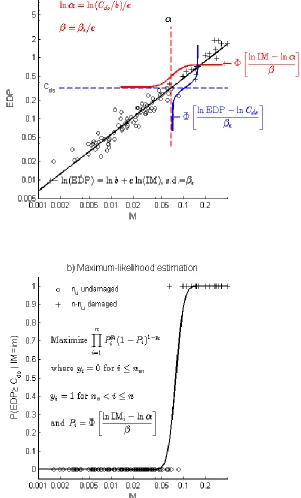
One widely-used method to estimate the probabilistic relation between the parameters EDP and IM is to perform a LS regression on the results of dynamic analyses (e.g. Cornell et al., 2002; Ellingwood and Kinali, 2009), assuming a lognormal distribution (Shome and Cornell, 1999). The predicted demand parameter is represented by a power law, with βε

being the standard-deviation of the error term of the logarithm of the predicted demand parameter (see Figure 1). Parallel developments have been made in the estimation of the parameters of fragility curves, based on MLE (e.g. Shinozuka et al., 2000), for which, like the LS approach, a lognormal distribution is usually assumed. The median and standard-deviation (respectively α and β) of the lognormal distribution are then estimated through the maximization of a likelihood function (see Figure 1b). Finally, similarly to MLE, an approach based on SSE has been investigated by Baker (2013), where the function to minimize is defined as follows, using the same notations as in Figure 1:

(4)

(5)

MLE was originally used to develop fragility curves from empirical data, like post-earthquake observations of bridge damage (Shinozuka et al., 2000), as it requires only binary information (damage / no damage) and no drift calculations or estimates, which cannot be accurately obtained from post-earthquake field surveys (from which only residual drifts can be observed). Several studies have also used MLE to post-process the results of non-linear time-history analyses (e.g. Kim and Shinozuka, 2004; Zentner, 2010), directly switching from drift values to the corresponding binary outcomes in terms of damage states. The use of MLE in the latter context may seem counter-productive, as it results in the loss of information (i.e. the actual value of the computed drifts). This drawback, however, may turn into an advantage when the development of near-collapse or collapse fragility curves is considered (Baker, 2013) since in this case most computation codes may return unreliable results or may not even converge, thus making LS regression difficult to apply (e.g. Shome and Cornell, 2000). In addition, MLE does not assume a predefined relation between IM and EDP (e.g. a power law) unlike the LS approach, which may be useful in the case of poorly correlated or constrained dynamic results.

LS regression is an efficient way to establish a robust relation between EDP and IM with only a few data points, as it makes use of all the information contained in the simulation results. It is also possible to extrapolate the regression line to higher or lower IM values, when such levels are not covered by the time-history analyses, although extrapolation is generally not recommended since structural behavior may alter beyond the range covered by the available analyses. A drawback of this method is that the standard-deviation βε of the

Figure 1. (a) Schematic representation of the derivation of fragility curves using the considered approaches: (a) least-squares regression and (b) maximum-likelihood estimation when the damage threshold Cds is assumed to be exactly known (i.e. βds=0). b and c are coefficients of the power law connecting the EDP and the IM and n is the number of calculations.

techniques covered by Baker (2007) may be seen as more elaborate variants and they rely mostly on the scaling of ground-motion records, which is out of the scope of the present paper. Porter et al. (2007) also comprehensively review various techniques to derive fragility curves focusing on those used for experimental results, among which the closest one to the LS regression evaluated here is called “method A”. Other approaches reviewed by Porter et al. (2007) imply the use of expert judgment or the combination of both empirical and analytical data, which makes them difficult to apply in the present study.

TRIAL INVERSION PROCEDURE

To assess the reliability of fragility curves derived from a limited number of time-history analysis we undertake a series of inversions on simulated data. This procedure enables comparison between the computed estimates with the true fragility parameters; thus constituting an efficient means to evaluate the robustness of the three regression techniques as a function of the number of data points (i.e. dynamic analyses). This inversion procedure is broken down into the following steps.

(1) The initial fragility parameters α0 and β0 are set, along with the corresponding

relation: ( ) and a probabilistic damage threshold Cds is assumed. Therefore, the global standard deviation of the relation between

the IM and the damage state can be written as: .

(2) A set of n IM values are defined and the corresponding EDP values sampled based on the relation in step 1 and the corresponding error term ε. The n data points represent the n dynamic analyses that would yield the pairs (IM, EDP). The IMs are assumed to be applicable for all magnitude (M) and distance (R) and consequently for which all possible earthquakes scenarios and associated ground motions should be considered. Assuming uniform distributions of M and R and lognormal ground-motion variability leads to IMs that are lognormally distributed (this has been numerically verified using a large strong-motion database), which is what is assumed here with a sufficient standard deviation to cover the entire range of possible ground motions. The series of IMs are also chosen in a way that roughly half the points are below the damage threshold (Cds) and half above,

where the most use can made of the available data samples, as stressed by Kato et al. (2008) via their study of information entropy.

(3) Using the n pairs of IM-EDP values, fragility curves as defined in Equation 5 are derived, using the three regression techniques described in the previous section. The estimated fragility parameters and can then be compared to the “true”

ones, α0 and β0,tot.

(4) The steps 2 and 3 are repeated k times (k>>1) in order to obtain stable estimates of the errors and confidence intervals of the estimated fragility parameters.

Using the set of k fragility estimates, several metrics are computed to obtain objective measures of the accuracy of the fragility functions with respect to the number of data points. Intuitive indicators are the standard deviations of both and , which can be computed for the k pairs using a bootstrap technique (e.g. Efron and Tibshirani, 1993).

Thanks to the inversion procedure, the fragility parameters obtained from the simulated data points can also be compared to the original parameters α0 and β0. This feature can,

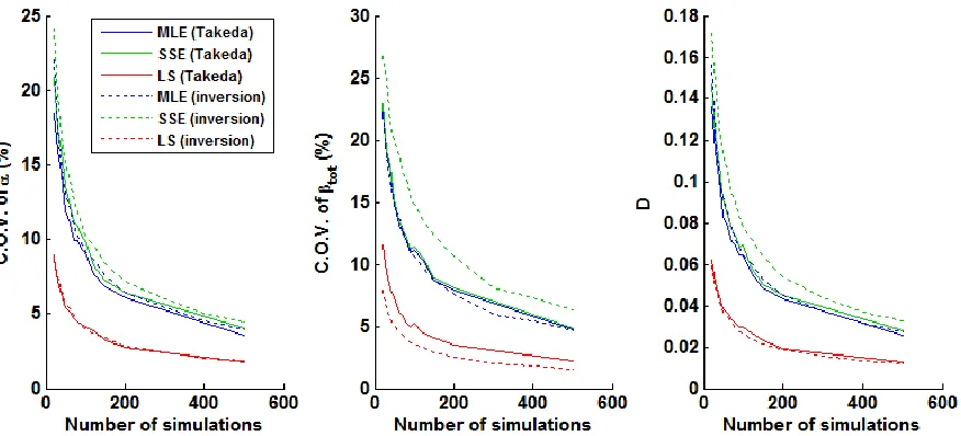
RESULTS AND IMPLICATIONS

The trial inversion procedure introduced above is carried out with k = 10 000 to obtain stable statistics. The following robustness indicators are computed for various numbers of data points (n ranging from 20 to 500) and for each of the three techniques (LS, MLE and SSE):

- Coefficients of variation (C.O.V., standard deviation divided by the mean) of the parameters and , to measure the precision of these terms;

- The mean of the Kolmogorov-Smirnov distance D over all k simulations, to compare the initial “true” distribution with the estimated one.

These results are presented in a series of graphs (see Figure 2) to show the evolution of each of the indicators with respect to the number of dynamic analyses. For the LS approach it is possible (e.g. Draper and Smith, 1981) to explicitly express the standard deviation of the terms ln b and c in the regression equation, based on the numbers of samples (i.e. n), the standard deviation of the regression and the distribution of the input variable (i.e. IM). Therefore an analytical estimation of the standard deviations of ln b and c has been performed and the C.O.V. of α and β have been evaluated using an error-propagation procedure (Ku, 1966). It is found that the analytical results are within 5% of the values obtained from the numerical approach, thus validating the results from the inversion procedure (See appendix A). These analytical estimations are valuable in checking the dispersion of the coefficients of the fragility curve (i.e. their precision) but they are not able to predict the accuracy of the curve, for which the Monte Carlo approach is required.

non-convergence of dynamic runs, when considering collapse or when analyzing post-earthquake observations).

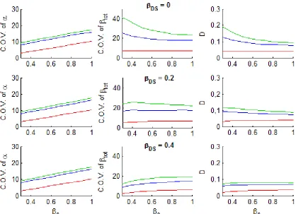
Figure 2. (Top left) Correspondence between the uncertainty on the fragility median α and the D metric. (Top right) Evolution of the uncertainty on α with the number of simulations. (Bottom left and right) Same construction for the fragility standard deviation βtot. The results from the three regression

techniques (respectively MLE, SSE and LS) are plotted in blue, green and red.

The introduction of an additional uncertainty in the definition of DS (i.e. βds) puts into

perspective the effect of the record-to-record variability, which is the focus here. Indeed, there is not much point in trying to obtain a perfect estimate of the structural response with respect to an IM, since other sources of variability, such as the damage state definition or modeling uncertainties, might be higher still and they would tend to dilute the effect of the variability due to the seismic input. It is worth noting that the uncertainties related to structural response calculation may be reduced by using more accurate structural models especially when dealing with a particular structure, while the record-to-record variability is related to the random nature of earthquake hazard.

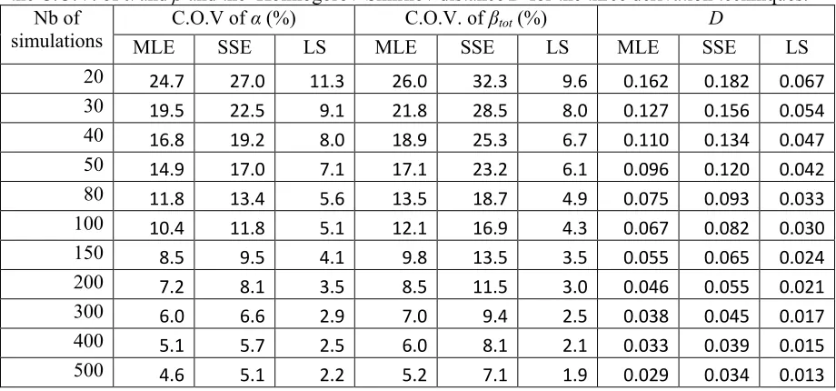
Table 1. Results from the inversion procedure, providing the link between the number of data points, the C.O.V. of α and β and the Kolmogorov-Smirnov distance D for the three derivation techniques.

Nb of simulations

C.O.V of α (%) C.O.V. of βtot (%) D

MLE SSE LS MLE SSE LS MLE SSE LS

20 _{24.7 27.0 11.3 26.0 32.3 9.6 0.162 0.182 0.067}

30 _{19.5 22.5 9.1 21.8 28.5 8.0 0.127 0.156 0.054}

40 _{16.8 19.2 8.0 18.9 25.3 6.7 0.110 0.134 0.047}

50 _{14.9 17.0 7.1 17.1 23.2 6.1 0.096 0.120 0.042}

80 _{11.8 13.4 5.6 13.5 18.7 4.9 0.075 0.093 0.033}

100 _{10.4 11.8 5.1 12.1 16.9 4.3 0.067 0.082 0.030}

150 _{8.5 9.5 4.1 9.8 13.5 3.5 0.055 0.065 0.024}

200 _{7.2 8.1 3.5 8.5 11.5 3.0 0.046 0.055 0.021}

300 _{6.0 6.6 2.9 7.0 9.4 2.5 0.038 0.045 0.017}

400 _{5.1 5.7 2.5 6.0 8.1 2.1 0.033 0.039 0.015}

500 _{4.6 5.1 2.2 5.2 7.1 1.9 0.029 0.034 0.013}

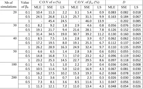
The results from Table 1 have been computed by selecting an initial standard deviation β0=0.5, which lies within the common range of dispersion for most fragility curves (e.g. standard deviations proposed within HAZUS; NIBS, 2004). A sensitivity study has also been conducted to check the effect of the standard deviation on the number of required simulations (see Table 2 and Figure 3). The calculations are performed for a range of β0 and three values

of βds. The following observations can be noted:

- For the three studied techniques, the value of βds has no effect on the precision of α,

- For the least-squares approach, the precision of βtot is roughly unchanged by β0 and

βds, although it decreases slightly (i.e. higher C.O.V.) as β0 increases for non-zero βds;

whereas for the other two approaches, the precision of βtot decreases (i.e. higher

C.O.V.) to a peak and then increases (i.e. lower C.O.V.) for non-zero βds whereas

when βds=0 the precision of βtot increases for increasing β0 (the reason for this

behavior is the interaction between the standard deviation of βtot and the value of βtot,

which equals );

- Because of the strong influence of the precision of βtot on the overall accuracy of the

fragility curve, the dependence of D on changes in β0 and βds is similar to the behavior

of the curves for C.O.V. of βtot, i.e. little impact of β0 and βds on the accuracy when

using least-squares, and generally increasing accuracy as β0 increases when using the

other two approaches.

Table 2. Evolution of the inversion results with the value of the initial standard deviation β0, for three sizes of datasets (50, 100 and 200 simulations)

Nb of simulations

Value of β0

C.O.V of α (%) C.O.V. of βtot (%) D

MLE SSE LS MLE SSE LS MLE SSE LS

20 0.1 10.4 11.3 2.2 3.1 5.4 0.9 0.083 0.082 0.018

0.5 24.5 26.8 11.3 25.7 31.5 9.9 0.163 0.184 0.067

1 - 45.4 24.5 - 46.0 13.9 - 0.202 0.085

30 0.1 8.2 9.2 1.8 2.9 4.6 0.8 0.056 0.076 0.014

0.5 19.1 21.7 9.4 21.6 28.1 7.8 0.126 0.152 0.055

1 31.4 34.5 19.0 30.7 39.2 11.2 0.130 0.160 0.069

40 0.1 8.5 7.5 1.6 2.8 3.9 0.7 0.062 0.062 0.013

0.5 17.2 19.5 8.0 19.1 25.3 6.7 0.112 0.137 0.047

1 26.2 28.9 16.3 24.9 32.4 9.7 0.110 0.135 0.059

50 0.1 6.6 6.5 1.4 2.8 3.8 0.6 0.051 0.055 0.011

0.5 14.8 16.8 7.1 17.0 23.2 6.2 0.096 0.119 0.042

1 23.2 25.3 14.5 22.7 29.5 8.6 0.097 0.118 0.052

100 0.1 4.5 5.1 1.0 2.2 2.9 0.4 0.036 0.041 0.008

0.5 10.5 11.6 5.0 12.0 16.9 4.3 0.067 0.081 0.030

1 16.2 17.5 10.2 15.3 19.3 6.2 0.068 0.078 0.037

200 0.1 3.2 3.6 0.7 1.6 2.3 0.3 0.026 0.030 0.006

0.5 7.3 8.1 3.6 8.5 11.6 3.1 0.047 0.056 0.021

Figure 3. (Left) Evolution of the C.O.V. of α with the value of β0, for the three regression techniques (i.e. MLE in blue, SSE in green and LS in red) and for a sample size of 100 simulations. (Middle) Evolution of the C.O.V. of βtot with the value of β0, for the three regression techniques and for a sample size of 100 simulations. (Right) Evolution of D with the value of β0, for the three regression techniques and for a sample size of 100 simulations.

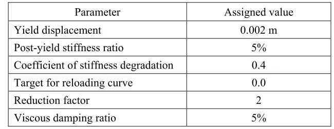
APPLICATION TO A SIMPLE STRUCTURAL MODEL

five-story (medium-rise) building. Standard values are assigned to the parameters describing the model (see Table 3).

To obtain a reference fragility curve – i.e. a “true” distribution – the first step consists in submitting the structure to a very large number of records. Since there are not enough natural ground motions in existing strong-motion databases, a set of synthetic ground motions was generated using the non-stationary stochastic procedure proposed by Pousse et al. (2006). These signals have been generated for magnitudes (Mw) between 5.5 and 7.5 and epicentral distances between 10 and 100 km. The five Eurocode-8 soil classes are also sampled to introduce additional variability in the ground-motion input. Around 100 000 of these records are generated and applied to the simplified model to obtain a well-constrained estimate of the structural response and its distribution. It is found that the IMs of the generated ground motions follow a lognormal distribution, as assumed earlier for the inversion. An arbitrary drift threshold is assumed so that approximately half the simulations are below and the other half above it (i.e. Cds = 0.16% for drift ratio – note that this does not necessarily correspond

to any particular damage state).

Table 3. Parameters of the modified Takeda model of the studied structure.

Parameter Assigned value

Yield displacement 0.002 m

Post-yield stiffness ratio 5%

Coefficient of stiffness degradation 0.4

Target for reloading curve 0.0

Reduction factor 2

Viscous damping ratio 5%

Using the LS regression approach, the high number of simulations gives us high confidence in the estimated fragility parameters (i.e. probability of exceeding the threshold Cds givenIM, taken as PSA at 0.5s): α0,LS =1.962 m/s² and β0,LS =0.400. However, it can be

using all simulation results; it is found α0,MLE =1.846 m/s² and β0,MLE =0.418, and α0,SSE =1.863 m/s² and β0,SSE =0.400 respectively. These are the parameters that are the basis of the comparisons to the successive fragility estimates, for both the MLE and SSE techniques.

Figure 4. Correlation between the 100 000 drift values from the Takeda model and the chosen IM [PSA (0.5s)].

The series of 100 000 simulation results is then used to randomly select subsets of IM-EDP couples, their sizes ranging from 100 to 1 000. For each subset size, 10 000 samplings with replacement are carried out (i.e. a bootstrapping technique) to obtain stable statistics on the estimates of fragility parameters. The different metrics described in the previous section are then computed to measure the performance of the different fragility derivation approaches (LS, MLE and SSE) for the different sample sizes and to check whether the results obtained with this structural model confirm the generic findings from the trial inversion procedure. In order to be consistent with the issue of dependence on the value of β0, the results are

compared with the ones of the inversion procedure carried out for β0=0.4 (see Figure 5).

Finally, the computed series of β, as well as the initial β0, are combined with βds = 0.4 to

Figure 5. Comparison of the evolution of the considered metrics with the number of simulations, between the theoretical inversion (solid line) and the Takeda model application (dotted line)

As it can be seen in Figure 5, all metrics vary with the number of simulations in accordance with the theoretical inversion. In the case of the LS regression approach, a good agreement with the theoretical findings is found and the metrics estimated through the inversion procedure are still slightly better than the ones obtained from the numerical model. This observation is in line with the assumption that the inversion procedure is based on a true power law with a constant dispersion, thus representing the ideal case. On the other hand, for the SSE method, the application results are a little less consistent with the theoretical ones, even though there are still quite close. The reason for this slight discrepancy is thought to be because of the nonlinear relation between the IM and drift and also the non-uniform dispersion (Figure 4) in contrast to the assumptions made when developing the theoretical results. Moreover, the assumed threshold for the drift does not split all results into exactly two equivalent sets (above and below the threshold), which is the ideal case for MLE and SSE techniques.

huge number of runs that is needed to get an estimate of the “true” distribution (i.e. around 100 000, as explained above) prevents the use of a MDOF model for this validation example.

CONCLUSIONS

ACKNOWLEDGEMENTS

The work presented here was performed in the framework of the ‘Multi-risks and Vulnerability’ research program of BRGM, including the EDF/BRGM-funded MARS project, the ANR-funded EVSIM project and the FP7-funded PERPETUATE project. We thank Jack Baker for sending us his recent paper on fitting fragility curves. The authors are very grateful to Prof. Peter Stafford for his constructive comments on an earlier version of this work and three anonymous reviewers for their detailed reviews of this article, which significantly improved the study.

REFERENCES

Applied Technology Council (ATC), 1996. Seismic evaluation and retrofit of concrete buildings. Report No. ATC-40, Redwood City, CA.

Applied Technology Council (ATC), 2011. Seismic performance assessment of buildings. Report No. ATC-58, Redwood City, CA.

Baker, J., 2007. Probabilistic structural response assessment using vector-valued intensity measures. Earthquake Engineering and Structural Dynamics36, 1861-83.

Baker, J., 2013, Efficient analytical fragility function fitting using dynamic structural analysis, Earthquake Spectra, submitted.

Bommer J.J., Magenes G., Hancock J., and Penazzo P., 2004. The influence of strong-motion duration on the seismic response of masonry structures. Bulletin of Earthquake Engineering

2(1):1–26

Buratti, N., Stafford, P. J., and Bommer, J. J., 2011, Earthquake accelerogram selection and scaling procedures for estimating the distribution of drift response. Journal of Structural Engineering (ASCE), 137(3), 345-357. doi: 10.1061/(ASCE)ST.1943-541X.0000217

Calvi, G.M., Pinho, R., Magenes, G., Bommer, J.J., Restrepo-Velez, L.F., and Crowley, H., 2006. Development of seismic vulnerability assessment methodologies over the past 30 years. ISET Journal of Earthquake Technology43, 75–104.

Carausu, A., and Vulpe, A., 1996. Fragility estimation for seismically isolated nuclear structures by high confidence low probability of failure values and bilinear regression. Nuclear Engineering and Design160, 287–297.

Cornell, C.A., Jalayer, F., Hamburger, R.O., and Foutch, D.A., 2002. Probabilistic basis for 2000 SAC Federal Emergency Management Agency steel moment frame guidelines. Journal of Structural Engineering 128(4), 526–533.

Draper, N. R., and Smith, H., 1981. Applied Regression Analysis, Second Ed., Wiley, New York.

Eads, L., Miranda, E., Krawinkler, H., and Lignos, D. G., 2013, An efficient method for estimating the collapse risk of structures in seismic regions, Earthquake Engineering and Structural Dynamics, 42(1), 25-41, DOI: 10.1002/eqe.2191.

Efron, B., and Tibshirani, R. J., 1993. An Introduction to the Bootstrap, Chapman & Hall/CRC Monographs on Statistics & Applied Probability.

Ellingwood, B.R., and Kinali, K., 2009. Quantifying and communicating uncertainty in seismic risk assessment. Structural Safety31, 179–187, doi:10.1016/j.strusafe.2008.06.001.

Hancock, J., Bommer, J.J., and Stafford, P.J., 2008. Numbers of scaled and matched accelerograms required for inelastic dynamic analyses. Earthquake Engineering and Structural Dynamics,

37(14), 1585-1607, doi: 10.1002/eqe.827.

Gehl, P., Seyedi, D.M., and Douglas, J., 2013. Vector-valued fragility functions for seismic risk evaluation. Bulletin of Earthquake Engineering, 11(2), 365-384. DOI 10.1007/s10518-012-9402-7.

Karim, K. R., and Yamazaki, F., 2003. A simplified method of constructing fragility curves for highway bridges, Earthquake Engineering and Structural Dynamics, 32(10), 1603-1626. doi: 10.1002/eqe.291.

Kato, M., Takata, T., and Yamaguchi, A., 2008. Effective updating process of seismic fragilities using Bayesian method and information entropy. Proceedings of the Japan-Korean Symposium on Nuclear Thermal Hydraulics and Safety, Okinawa, Japan, N6P1036.

Kennedy, R.P., Cornell, C.A., Campbell, R.D., Kaplan, S., and Perla, H.F., 1980. Probabilistic seismic safety study of an existing nuclear power plant. Nuclear Engineering and Design59, 315-338.

Kim, S.H., and Shinozuka, M., 2004. Development of fragility curves of bridges retrofitted by column jacketing. Probabilistic Engineering Mechanics19, 105–12.

Ku, H. H., 1966. Notes on the use of propagation of error formulas, Journal of Research of the National Bureau of Standards – C. Engineering and Instrumentation, 70C(4), 263-273.

Lestuzzi, P., Belmouden, Y., and Trueb, M., 2007. Non-linear seismic behavior of structures with limited hysteretic energy dissipation capacity. Bulletin of Earthquake Engineering5(4), 549-569.

Moehle, J., and Deierlein, G.G., 2004. A framework methodology for performance-based earthquake engineering. Proceedings of the 13th _{World Conference on Earthquake Engineering, Paper n°679,}

Vancouver, B.C., Canada.

NIBS. 2004. HAZUS-MH: Users’s Manual and Technical Manuals. Federal Emergency Management Agency, Washington, D.C.

Otani, A., 1974. Inelastic analysis of R/C frame structures. Journal of Structural Division, ASCE

100(ST7), 1433–1449.

Pacific Earthquake Engineering Research Center (PEER), 2009. Evaluation of Ground Motion Selection and Modification Methods: Predicting Median Interstory Drift Response of Buildings, Haselton, C. B. (editor), PEER Report 2009/01, PEER Ground Motion Selection and Modification Working Group, University of California, Berkeley.

Porter, K., Kennedy, R., and Bachman, R., 2007. Creating fragility functions for performance-based earthquake engineering. Earthquake Spectra23(2), 471-489.

Pousse, G., Bonilla, L.F., Cotton, F., and Margerin, L., 2006. Non stationary stochastic simulation of strong ground motion time histories including natural variability: Application to the K-net Japanese database. Bulletin of Seismological Society of America96(6), 2103-2117.

Saez, E., Lopez-Caballero, F., and Modaressi-Farahman-Razavi, A., 2011. Effect of the inelastic dynamics soil-structure interaction on the seismic vulnerability assessment. Structural Safety33, 51–63, doi: 10.1016/j.strusafe.2010.05.004.

Schwab, P., and Lestuzzi, P., 2007. Assessment of the seismic non-linear behaviour of ductile wall structures due to synthetics earthquakes. Bulletin of Earthquake Engineering5(1), 67-84.

Shinozuka, M., Feng, Q., Lee, J., and Naganuma, T., 2000. Statistical analysis of fragility curves. Journal of Engineering Mechanics126(12), 1224–31.

Shome, N., and Cornell, C.A., 1999. Probabilistic seismic demand analysis of nonlinear structures. Tech. Rep. RMS–35, RMS Program, Stanford University, CA.

Shome, N., and Cornell, C.A., 2000. Structural seismic demand analysis: Consideration of “Collapse”. Proceedings of the 8th ASCE Specialty Conference on Probabilistic Mechanics and Structural Reliability, Paper n°119.

Shome, N., Cornell, C. A., Bazzurro, P. and Carballo, J. E., 1998, Earthquakes, records, and nonlinear responses, Earthquake Spectra, 14(3), 469-500.

Vamvatsikos, D. and Cornell, C.A., 2002. Incremental dynamic analysis. Earthquake Engineering and Structural Dynamics31, 491–514. doi: 10.1002/eqe.141.

Appendix A – Analytical verification of error terms

The assumed relationship between EDP and IM is:

(A1)

The standard deviations of the coefficients in equation A1 are (Draper and Smith, 1981):

(A2)

(A3)

Considering the variable change for the LS regression we have (See Figure 1):

_(A4)

(A5)

In order to estimate error propagation in calculating lnα and ß using equations (A4) and (A5), the following equation is used (Ku, 1966):

(A6)

where sf is the standard deviation of the function f, si stands for the standard deviation of

variable i and ρi,j represents the covariance term between variables i and j. The standard

deviations of lnα and β are then estimated as:

(A7)

(A8)

Finally, σlnα is translated to σα through the following relation: . (A9)

A comparison between numerical standard deviations of lnα and β (obtained through the inversion procedure with the LS approach) and analytical ones (estimated by equations A8 and A9) is presented in table A1, considering the following parameters: βε = 0.5, b = 1, c = 1

and Cds = 0.02. It can be seen that the analytical results are within 6% of the values obtained from the numerical approach.

Nb of simulations

Inversion results Analytical results Difference on

σα σβ σα σβ σα σβ

50 0.00144 0.0503 0.001446 0.052618 0.4% 4.6%

100 0.00102 0.0349 0.001012 0.036851 -0.8% 5.6%

150 0.00082 0.0287 0.000824 0.030373 0.4% 5.8%

200 0.00071 0.0254 0.000712 0.026860 0.3% 5.7%

300 0.00058 0.0207 0.000580 0.021944 0.1% 6.0%