Inspection and crime prevention:
an evolutionary perspective
Vassili Kolokoltsov1, Hemant Passi2, Wei Yang3Abstract
In this paper, we analyse inspection games with an evolutionary perspective. In our evolutionary inspection game with a large pop-ulation, each individual is not a rational payoff maximiser, but pe-riodically updates his strategy if he perceives that other individuals’ strategies are more successful than his own, namely strategies are sub-ject to the evolutionary pressure. We develop this game into a few directions. Firstly, social norms are incorporated into the game and we analyse how social norms may influence individuals’ propensity to engage in criminal behaviour. Secondly, a forward-looking inspector is considered, namely, the inspector chooses the level of law enforcement whilst taking into account the effect that this choice will have on future crime rates. Finally, the game is extended to the one with continuous strategy spaces.
Key words: inspection game, social norms, crime rate, law enforcement
1
Introduction
An inspection game is a non-cooperative game whose players are often called an inspector and an inspectee. It models a situation where the inspectee, which may be an individual, an organisation, a state or a country, is obliged to follow certain regulations but has an incentive to violate them. The inspector tries to minimise the impact of such violations by means of in-spections that uncover them. Typically an inspection game has a mixed equilibrium.
Inspection games have a wide variety of applications including arms control [12, 10, 11, 39], auditing of accounts [41, 19, 20], tax inspection
1
Department of Statistics, University of Warwick, Coventry, CV4 7AL, UK, v.kolokoltsov@warwick.ac.uk
2
New Zealand Treasury Wellington, 6011, New Zealand, he-mant.passi@treasury.govt.nz
3
Department of Mathematics and Statistics, University of Strathclyde, Glasgow, G1 1XH, UK, w.yang@strath.ac.uk
[58, 54, 37, 51, 50, 1], environmental protection [56, 67, 38, 6], quality con-trol in supply chains [52, 61, 40], stockkeeping [27] and communication in-frastructures [34, 23]. Some of these are surveyed in e.g. [15, 7, 12, 16]. The research on inspection games can contribute to the construction of an effective inspection plan for the inspector when an illegal action is executed strategically.
This subject has been investigated quite extensively during the last five decades. Still, it continues to draw attention. Throughout the 1960s and the three decades that ensured, the underlying motivation was the cold war between the US and the Soviet Union and the desire to monitor the various arms control agreements that were signed by the two superpowers. Ana-lytically, these settings led quite naturally to two-person game formulations with various assumptions about the strategy sets that were feasible to each of the two parties. Since the early 1990s, attention has shifted to other di-rections and new circumstances require moving from two-person to n-person formulations, from zero-sum games to non-zero-sums.
In the initial work done by Dresher [26] and Kuhn [43], they considered sequential inspection games for the treaty of arms reduction where one player wishes to violate the treaty in secret while the other player makes a plan for inspection. In a sequential inspection game, an inspector has to distribute a given number of inspections over a larger number of inspection periods in order to detect an illegal act that an inspectee, who can count the inspector’s visits, performs in at most one of these periods. Maschler [46] generalized Dresher’s modelling. In Maschler’s model, the inspectee (violator) must pay a unit penalty if the violation is exposed by an inspection, but he can escape the exposure by a side payment of penalty γ. Dresher discusses special cases of γ = 1/2 and γ = 1, and Maschler considered the general case 0≤γ ≤1. Diamond [25] and Ruckle [55] also studied two-person zero-sum games between an inspector and an inspectee and a pair of equilibrium strategies was sought.
In the setting of inspections by the customs against smugglers, Thomas and Nisgav [63] extended Maschler’s model to a game in which customs keeps watch on illegal actions of a smuggler by using one or two patrol boats, and the number of boats affects the reward obtained on the capture of the smuggler. They formulated the problem as a multi-stage game, and adopted a numerical method where a one-stage matrix game is repeatedly solved.
inspectee (violators or smugglers) when both players meet. They assumed that the capture probability depends on the number of patrol boats. Ger-naev [33] extended Baston and Bostock’s work to a model with three patrol boats. Sakaguchi [60] and Von Stengel [65] studied inspection games with several smuggling opportunities in a perfect-capture model. Ferguson and Melolidakis [31] extended further this model by assuming that the smuggler can avoid capture by paying some cost γ ≤ 1. If he is captured on his smuggling, the smuggler must pay unit cost.
Since the inspection resources (inspection personnel, equipments or time) are usually limited and complete surveillance is not possible, it is natural to include the first kind error (probability of a false alarm) α given that the inspectee acts legally and the second kind error (probability of non-detection) β that no alarm is raised given that the inspectee acts illegally. This kind inspection game is referred to as an imperfect inspection game, see e.g. Rothenstein and Zamir [53], Canty, Rothenstein and Avenhaus [22]. Rothenstein and Zamir [53] extended Diamond’s model [25] by including fixed errors of the first and second kind for a single inspection. Canty, Rothenstein and Avenhaus [22] solved a non-sequential inspection game with first and second kind errors based on a fixed detection time goal and obtained some special solutions for the sequential case.
It is worth noting that the papers cited above study zero-sum inspection games. However under certain circumstances, one cannot justify the zero-sum aszero-sumption and non-zero-zero-sum formulations are presented, e.g. in Aven-haus and von Stengel [14], AvenAven-haus, Von Stengel and Zamir [16], AvenAven-haus [8], Avenhaus and Canty [9], Kolokoltsov and Malafeyev [42], Avenhaus and Kilgour [13], Hohzaki [39] and Deutsch, Golany and Rothblum [24].
Avenhaus [8], Kolokoltsov and Malafeyev [42] presented a one-inspector-one-inspectee non-zero-sum one-step imperfect inspection game, where the inspector has a non-detection probability β. Avenhaus and Canty [9] con-sidered a similar model in a sequential setting, and subject to both kind errors. In these works, they gave an explicit form of the unique Nash equi-librium of this game, i.e. a mixed strategy profile (p∗, q∗), where p∗ is the optimal probability with which the inspector inspects andq∗ is the optimal probability with which the inspectee acts illegally.
are solved separately and the solution of one game is a parameter of the sec-ond game. First, assuming that the inspectee acts illegally, they formulated a zero-sum game where the inspector faces a hypothesis testing problem δ and the inspectee chooses an optimal violation mechanismω. That is, for any test δ, the inspectee will choose a violation mechanismω∗ to maximise the non-detection probabilityβ(δ, ω). On the side of the inspector, first he chooses a fixed false alarm probability α and consider only those tests that result in this error probability. Then he will choose a testδ∗ that minimizes the worst-case non-detection probability β(δ∗, ω∗). Namely, in equilibrium, the non-detection probability is represented byβ(α) := minδmaxωβ(δ, ω).
Then they solved the original non-zero-sum game to get the optimal false alarmα∗for the inspector and optimal probabilityq∗for the inspectee acting illegally.
Avenhaus and Kilgour [13] studied a one-inspector-two-inspectees non-zero-sum inspection game with imperfect inspections. They found a Nash equilibrium where the inspector divides his inspection effort among two in-spectees. Further, they showed that when detection functions (probability of detecting), as functions of inspection effort, are convex, inspection effort should be concentrated on one inspectee chosen at random, but when de-tection functions are concave it should be spread deterministically over the inspectees.
Hohzaki [39] extended Avenhaus and Kilgour’s model [13] to a one-inspector-n-inspectees non-zero-sum inspection game, where the inspectee k,k∈[1, n], has lk facilities which are set as targets for the inspection and
the inspector has a budget constraintC >0. He decomposed this non-zero-sum inspection game into two optimisation problems: an optimal assignment problem of inspection staff and an optimal division problem of the budget. For an optimal assignment problem of inspection staff, he started with as-suming resource yk is assigned to the inspectee k, with
Pn
k=1yk =C. An
feasible assignment plan of the inspection staff xk = {xki ≥ 0, i = 1, .., lk}
must satisfy Plk
i=1ckixki =yk, then the inspector aims to minimise the
non-detection probability β(yk) over feasible assignment plans xk, k ∈ [1, n].
Further, knowing the minimum non-detection probability β∗(yk), he
ob-tained a Nash equilibrium (y∗ = {y∗1, . . . , y∗n}, q∗ = {q1∗, . . . , qn∗}) of pure strategies of the inspector and mixed strategies of the inspectees by solving an optimal division problem of the budget. Deutsch, Golany and Rothblum [24] considered a similar non-zero-sum game with single inspector multiple inspectees and provided closed-form expressions of Nash equilibria.
Avenhaus [8], Kolokoltsov and Malafeyev [42] tom-inspectors-n-inspectees one-step non-zero sum games. In this game, they assumed theminspectors are uncoordinated and theninspectees are non-interacting. Inspectors have probability p to perform the inspection. If an inspector decides for the in-spection, then the inspection will be performed on a single randomly chosen inspectee. Given the inspection, each inspectee will have probability 1/2 to be inspected. The inspectees have respectively probabilitiesq1, . . . , qnof
act-ing illegally. They provided explicit form of mixed strategies (p∗, q∗1, . . . , q∗n) for these games.
In the setting of production economics, inspection games are modified in the way that a third player, symbolizing a mediator and coordinating the inspector and the inspectee, is introduced to guarantee that the inspector and the inspectee behave in accordance with the objectives of the firm. For detailed discussion, see e.g. Borch [19], Anderson and Young [3], Avenhaus, Von Stengel and Zamir [16], Fandel/Trockel [28], Fandel/Trockel [29, 30]. Another direction of modification of inspection games is to consider the inspector as a Stackelberg leader of the game, see more e.g. in Andreozzi [5, 4]. McEneaney and Singh [47] studied inspections with spatially nontrivial distributions. A very much related model to the inspection game is the
patrolling game which involves the scheduling and deployment of patrols, for discussions on the patrolling game see e.g. [2] and references therein.
Inspection games are also applied to law enforcement. Tsebelis [64] first used inspection games to model phenomena in criminal justice. According to Tsebelis [64], modifying the size of the penalty does not affect the fre-quency of crime commitment at equilibrium, but rather the frefre-quency of law enforcement. Pradiptyo [48] refined the inspection game proposed by Tesbelis, by using empirical evidence from various studies, which primarily conducted in the UK, to re-construct the game. They found that an increase in the severity of punishment will reduce the likelihood of the enforcement of the law. Instead of increasing the severity of punishment, theoretically, the authority may reduce individuals’ offending behaviour by providing finan-cial compensation to those who do not have criminal records. This is widely known as crime prevention initiative. Interesting psychological analysis of the logic and rationale employed by the players in such game scenarios can be found in Rauhut [49]. Altruistic punishment in promoting cooperation in a large population can be found e.g. in [59] and [32] and many references therein.
full-time or does not work at all. Each individual chooses to work if and only if his choice results in higher utility than living off the transfer, i.e.
u[(1−a)w]> u(b) +µ−v(x),
where u : [0,∞) → [0,∞) is the utility function, a ∈ (0,1) is the tax rate, b ∈ R+ is the amount of government transfer, w ∈ [0,∞) is the wage, x ∈ [0,1] is the population share living on the transfer, v(x) is a decreasing function describing the disutility from accepting the transfer, µ is the utility difference between the leisure of living on the transfer and the intrinsic utility that one may derive from work life. They proved that for every tax rate a∈(0,1), transfer b∈[0,∞) and expected population share x∈[0,1] of the transfer recipients, there exists a unique critical wage ratew∗ such that all individuals with lower wages than w∗ choose not to work and those with higher wages than w∗ choose to work. Further, an equilibrium population sharex∗ ∈[0,1] of transfer recipients can be obtained by solving the equation
x= Φ
u−1[u(b) +µ−v(x)] 1−a
where Φ : [0,∞)→ [0,1] is a continuously differentiable cumulative proba-bility distribution function of wages for each individual andu−1denotes the inverse function of u. By considering the so-called government balance re-quirement, that is public transfer spending is equal to public revenues from the wage tax, they showed some interesting observations on the relation between the tax rateaand the transfer b.
2
A conventional inspection game
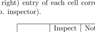
In its simplest form, an inspection game is a two-player game between an individual (i.e. inspected) and an inspector. The individual must choose whether to violate or comply with the wishes of the inspector, who himself must decide whether to inspect the individual or not. Each player makes his strategy choice without observing that of the other. This situation can be illustrated as the following 2x2 normal form game in Table 1, where the individual is the row player and the inspector is the column player, and the left (resp. right) entry of each cell corresponds to the payoffs for the individual (resp. inspector).
Inspect Not Inspect
Violate −1,1 2,−2
[image:7.612.172.338.252.308.2]Comply 0,−1 0,0
Table 1: The simplest two-player inspection game
The key feature of an inspection game is that the interests of the in-dividual clash with those of the inspector. The inspector would obviously prefer the individual to comply, but would rather not have to inspect. How-ever, if the inspector chooses not to inspect, the individual would always prefer to violate. As a result of this conflict, an inspection game contains no pure strategy Nash equilibria: whatever the outcome of the game, either the individual or the inspector would always want to switch their strategy to something that would upset their opponent, who in turn would wish to switch their strategy and so on...
This element of strategic indeterminacy is resolved by resorting to mixed strategies, whereby at least one player randomises over his pure strategies. In fact it is straightforward to show that the unique Nash equilibrium of an inspection game involves both players choosing to play mixed strategies, therefore implying that both inspection and non-compliance occur with pos-itive probabilities.
basic notations:
r=legal income received by the individual if he complies, r >0 l=crimial profit received by the individual if he violates without
being caught, l >0
f =fine paid by the individual if he violates and is caught, f >0
c=cost for the inspector to inspect, c >0
λ=the probability with which the individual is caught if the inspector inspects, λ∈(0,1)
In a general form of the inspection game between an individual and an inspector can be described as follows: if the individual abides by the law then he receives the legal incomer, whereas the payoff to the individual that violates depends on the strategy chosen by the inspector. If the inspector did not inspect, the individual escapes with his legal incomer plus criminal profitsl. However if the inspector did inspect, then the individual is either caught with a probability λ and has to pay the fine f, or escapes with a probability 1−λand the criminal profits l. The parameter λcan also be interpreted as the efficiency of inspection.
Meanwhile, the inspector must incur the fixed costcin order to inspect. If the individual played Comply, this expense is sunk, and the individual receives no further payoff. However, if the individual chose to violate, then the inspector may catch the individual with the probability λand earn the fine f, otherwise the individual escapes, causing the inspector lossesl. On the other hand, if the inspector chose not to inspect, he sustains losses l when the individual plays Violate, and 0 when the individual plays Comply.
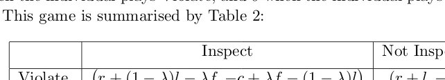
This game is summarised by Table 2:
Inspect Not Inspect
Violate r+ (1−λ)l−λf,−c+λf−(1−λ)l (r+l,−l)
[image:8.612.97.418.484.542.2]Comply (r,−c) (r,0)
Table 2: a general inspection game
In order to ensure that the game can be interpreted as a conventional inspection game, very often the following two additional restrictions on the payoffs are imposed:
and
λf >(1−λ)l. (2.2)
Restriction (2.1) states that, given that the individual is violating, the in-spector prefers to inspect since the expected benefit from inspecting exceeds the cost. Restriction (2.2) states that, given the inspector is inspecting, the individual prefers not to violate since the expected fine exceeds the expected criminal profit.
The following theorem gives the unique Nash equilibrium of this game and was proved in [42] .
Theorem 2.1. Let p ∈ [0,1] be the probability with which the individual violates and q ∈ [0,1] be the probability with which the inspector inspects. The unique Nash equilibrium of the two-player inspection game described in Table 2 is the mixed strategy profile (p∗, q∗) with
p∗ = c
λ(l+f) and q
∗ = l
λ(l+f).
3
An evolutionary inspection game
In this section, we consider an inspection game with a large population of interacting individuals and a single inspector. In this game, we do not assume that individuals know all relevant features of the game and maximise their payoffs accordingly. Instead, we will replace this conventional payoff maximisation with the idea that individuals modify their strategies after observing the experiences of others. The proportion of individuals who play a particular strategy is then subject to evolutionary pressure over time such that the population share of better performing strategies increases and that of strategies earning lower payoffs decreases. We refer to this model as an evolutionary inspection game. The key feature of this evolutionary inspection game is that the transmission process by which the strategies of Violate and Comply propagate is fundamentally social in nature.
3.1 Basic model of an evolutionary inspection game
The fraction of violators in the population is
p: [0,∞)→[0,1], t→pt.
The valuept, called thecrime rate at timet, can also be understood as the
probability with which each individual violates at timet.
The fraction of the population that is inspected by the inspector is
q : [0,∞)→[0,1], t→qt.
The value qt, called the level of law enforcement at time t, can also be
understood as the probability with which each individual is inspected. The cost function of law enforcement for the inspector is
F : [0,1]7→[0,∞), q→F(q),
withF(0) = 0 (that is, the cost of zero inspection is zero).
At any timet∈[0,∞), a complier always receives the legal incomerwith certainty, so for any given level of law enforcement qt, a complier expects
the payoff:
πC(t) =:E[UI(C, qt)] =r. (3.1)
where UI(C, q) denotes the utility of a complier with any level of law
en-forcementq ∈[0,1].
At any time t∈ [0,∞), if an individual violates, the infraction may go unnoticed with the probability 1−λqt and the violator escapes with the
criminal profitsl; otherwise the violator is caught with the probabilityλqt
and punished with a fine f. Therefore a violator expects the payoff:
πV(t) =:E[UI(V, qt)] =r+ (1−λqt)l−λqtf. (3.2)
where UI(V, q) denotes the utility of a violator with any law enforcement
q∈[0,1].
At any timet∈[0,∞), roughly speaking there will be N pt violators, of
which a fraction ofλqtis expected to be caught and 1−λqtto escape. Those
who are caught have to pay the fine f to the inspector whereas those who escape cause a loss l for the inspector. Formally, at time t, the inspector expects the payoff:
E[UA(qt, pt)] =−F(qt) +N ptλqtf −N pt(1−λpt)l (3.3)
where UA(q, p) denoted the utility of the inspector who has a law
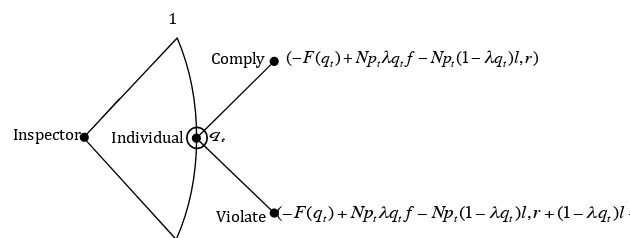
Inspector
0
Violate Comply
Individual 1
(−F(qt)+Nptλqtf−Npt(1−λqt)l,r)
qt
[image:11.612.97.412.98.217.2](−F(qt)+Nptλqtf−Npt(1−λqt)l,r+(1−λqt)l−λqtf)
Figure 1: The extensive form of the evolutionary inspection game
The above analysis can be summarised in Figure 1:
In order to ensure that the game does not degenerate, we impose the following restriction on the payoff of the individual: if the inspector inspects with certainty, the individual prefers not to violate, i.e.
Assumption(A1) (1−λ)l < λf. (3.4)
Inequality (3.4) is the same as the restriction (2.2) in the canonical setting. In an evolutionary setting, each individual playsV orC as a fixed strat-egy for a certain period, and then periodically updates his stratstrat-egy. At the beginning of each period, some exogenous and fixed fraction ω ∈ [0,1] of the population can update their behaviour upon meeting another randomly chosen individual in the population. If two individuals meet and have the same strategy, then that strategy is retained by the updating individual. If however, the two individuals have different strategies, the updating individ-ual may revise his behaviour on the basis of the payoffs enjoyed by the two in the previous period.
More specifically, at a given time t ∈ [0,∞), the fraction 1−pt of the
population are compliers andω of these are in an updating mode and called
compliant updaters. Among these compliant updaters, a fractionptof them
then meet violators. If the payoff from violating exceeds that from com-plying, i.e. πV(t) > πC(t), the compliant updater will switch his behaviour
with the switching probability
β(πV(t)−πC(t))
compliant updater does not switch. The coefficient β reflects the greater effect on switching of relatively large payoff differences.
The fraction of violators in the next period is equal to the fraction ptof
violators in the previous period, plus the fraction of compliers who convert to violators, and minus the fraction of violators who convert to compliers. Formally the population frequency of violators, at timet+ ∆t(∆t >0), can be written as
E[pt+∆t] =pt+ωpt(1−pt)IV >Cβ(πV(t)−πC(t))∆t
−ωpt(1−pt)IC>Vβ(πC(t)−πV(t))∆t
(3.5)
where IV >C (resp. IC>V) is an indicator function that equals to one if
πV(t) > πC(t) (resp. πC(t)> πV(t)) and zero otherwise. Since the
popula-tion is sufficiently large, we can replaceE[pt+∆t] by pt+∆t and get
pt+∆t=pt+ωβpt(πV(t)−π¯(t))∆t (3.6)
where
¯
π(t) =ptπV(t) + (1−pt)πC(t) (3.7)
is the average payoff at time t for the population as a whole. Subtracting pt from both sides of equation (3.6), dividing by ∆tand taking the limit as
∆t → 0, one gets the well-known replicator equation (cf. e.g. Taylor and Jonker [62] or Zeeman [68])
˙ pt=
dpt
dt =ωβpt(πV(t)−π¯(t)). (3.8) This equation states that the growth rate of the fraction of violators is proportional to the amount by which the payoff from violating exceeds that from complying.
By (3.2), (3.7) and (3.1), we can rewrite (3.8) and derive a replicator equation for the frequency of violators in the population, which is presented in the following.
Proposition 3.1. In an evolutionary inspection game with a large popula-tion of individuals, the replicator equapopula-tion for the frequency of violators is given by
˙
pt=ωβpt(1−pt)(l−λqt(l+f)). (3.9)
of crime pt and law-enforcement qt. In fact, individuals need not even be
aware of the overall levels of crime and law-enforcement. Instead, individ-uals periodically meet with other members of the population, observe their strategies, and consider updating their behaviour if they perceive that other individuals’ strategies are more successful than their own.
The implications of the replicator dynamic are that although no indi-vidual can be considered to be a rational payoff maximiser, strategies are subject to the evolutionary pressure. In other words, strategies that are successful in terms of yielding above-average payoffs will propagate through the population by imitation. Therefore the replicator equation is said to be a payoff-monotonic dynamic.
Next, we will analyse how the inspector responds dynamically to the evolving level of crimept, t≥0. In this basic model of an evolutionary
in-spection game, we assume that the crime ratesptare visible for the inspector
and that the inspector plays a straightforward best-response to the visible crime rates. More specifically, at each time t≥ 0, the inspector takes the crime-rateptas given and tries to find a level of law enforcementqt so as to
maximise his expected payoff. Specifically, at each time t≥0 and given a crime ratept, the inspector aims to maximise his payoff (3.3), i.e.
max
qt∈[0,1]
{−F(qt) +N ptλqtf−N pt(1−λqt)l}. (3.10)
Remark 3.1. One may think that this straightforward best-response strat-egy is somewhat naive as it assumes that the inspector does not choose pt
strategically so as to influence future levels of crime rate. However, one can also consider the situation that, perhaps due to political or resource issues, the inspector may not trade-off non-best response strategy in the short-run in the pursuit of some long-run objectives. At any case, this simplifying as-sumption provides an interesting benchmark from which other asas-sumptions can be compared, see e.g. subsection 3.3.
Assumption (A2): The cost function F is twice continuously differen-tiable and
0< F0(q)≤N λ(l+f) andF00(q)>0, for all q∈[0,1],
where F0 and F00 denote the first-order and the second-order derivatives of
F, respectively.
crime ratep∈[0,1] is denoted by
ˆ
q[p] := arg max
q∈[0,1]{−F(q) +N pλqf−N p(1−λq)l}. (3.11) Define
¯
p:= min{p∈[0,1] : ˆq[p] = 1}.
Clearly for p ∈ [¯p,1], we have ˆq(p) = 1. Essentially, the assumption(A2) requires that there exists a critical level of crime rate ¯p ∈ (0,1] such that if the prevailing crime rate is higher than ¯p, the inspector will inspect with certainty.
A very basic example of the cost function F in our setting is
F(q) =αq2 (3.12)
with a constant 0< α≤ N λ(2l+f). In this case, the unique best-response for the inspector to crime ratep∈[0,1] is given by
ˆ
q[p] = min
N λ(f +l) 2α p,1
which is a linear function inp. The critical level of crime rate ¯pis given by
¯
p= 2α N λ(f +l).
We will keep this example in mind in the following analysis.
Proposition 3.2. Let assumptions (A1) and (A2) hold. Then the best-response function for the inspector
ˆ
q : (0,p¯)7→(0,1), p7→qˆ(p),
defined in (3.11), is strictly increasing in p.
Proof. By the definition of the best response function ˆq(·) in (3.11), we have the following first order condition
−F0(ˆq(p)) +N pλ(l+f) = 0 (3.13)
and the second order condition
are satisfied. Differentiating (3.13) with respect to p, together with (3.14), yields
dqˆ dp(p) =
N λ(l+f) F00(ˆq(p)) >0
which completes the proof.
Proposition (3.2) says that the inspector’s optimal level of law enforce-ment is increasing in the crime rate.
After having discussed the dynamics for both individuals and the in-spector, we are now in a position to analyse the qualitative behaviour of the system. Substituting (3.11) into (3.9), one gets that the fixed points of the replicator equation (3.9) occur atp∗= 0, p∗ = 1, andp∗ such that
ˆ
q(p∗) = l
λ(l+f). (3.15)
Clearly, by the assumption(A1), ˆq(p∗) in (3.15) is within (0,1). Since we have proved that ˆq(p) is strictly increasing in p in Proposition 3.2 , the solutionp∗ ∈(0,1) of (3.15) is unique, we refer to this fixed pointp∗ ∈(0,1) as theinterior fixed point of (3.9).
Theorem 3.1. Let assumptions (A1) and(A2) hold. Then
(i) The fixed points p∗ = 0 and p∗ = 1 of (3.9)are unstable.
(ii) There exists an unique stable interior equilibrium of the evolutionary inspection game (p∗, q∗) with
p∗ = 1 N λ(l+f)F
0( l
λ(l+f)) and q
∗ = l
λ(l+f).
Proof. To analyse the stability of the fixed points of this system, we apply the method of linearizing around these fixed points (c.f. [60]). Specifically, define a functionj: [0,1]7→R by
j(p) =ωβp(1−p) l−λqˆ(p)(l+f)). (3.16)
Let p∗ denote the fixed point of the system and ht := pt−p∗ be a small
perturbation away fromp∗. The linear equation
˙ ht=ht
dj dp(p
∗)
if dpdj(p∗) < 0 and unstable if dpdj(p∗) > 0. Differentiating the function j(p) (3.16) with respect top gives us
dj
dp(p) =ωβ(1−2p) (l−λqˆ(p)(l+f))−ωβλ dqˆ(p)
dp p(1−p)(l+f).
At the point p∗ = 0, we obtain
dj
dp(0) =ωβ[l−λqˆ(0)(l+f)] =l >0.
Therefore the fixed pointp∗= 0 is unstable.
In order to check whether there exists an interior point p∗ ∈ (0,1) and to determine the its’ value, we substitute (3.15) into the authorities’ first order condition (3.13). Together with the assumption (A2) we get p∗ =
F0(q∗)
N λ(l+f) ∈(0,1) whereq
∗ = l
λ(l+f) ∈(0,1) . For the stability of this interior fixed point, we have
dj dp(p
∗) =−ωβλdqˆ(p∗)
dp p
∗(1−p∗)(l+f)<0
since ˆq is increasing in p, i.e. dqˆdp(p) > 0 for any p ∈(0,p¯). Therefore, this interior fixed point is stable.
At the fixed pointp∗ = 1, we have
dj
dp(1) =−ωβ[l−λqˆ(1)(l+f)].
Since there exists an interior fixed point p∗ ∈ (0,1) such that ˆq(p∗) =
l
λ(l+f) ∈ (0,1), we have ˆq(1) ∈ (
l
λ(l+f),1], by Proposition 3.2. Therefore
dj
dp(1)>0, which implies the fixed pointp
∗ = 1 is unstable.
equilibrium marginal costs are F0(q∗). Comparing the expressions for p∗
and q∗ in Theorem 2.1 and Theorem 3.1, we can therefore see that their interpretations are essentially the same.
3.2 Crime and social norms
The key feature of an evolutionary inspection game is that the process of individual behavioural change is fundamentally social in nature. Given this position, it is not difficult to imagine applications where other social factors may also exert an influence on individuals’ decisions.
Abiding by the law is a social norm but the strength of this norm depends on the size of the population share that adheres to the law. A very low overall crime rate helps to foster a culture of honesty in the population which serves to reinforce individuals’ sense of moral responsibility. Conversely if crime is rife, individuals may begin to feel that breaking the law is socially acceptable.
In this subsection, we will incorporate social norms into our model and analyse how social norms may influence individuals’ propensity to engage in criminal behaviour. Inspired by the work [44], we model social influence as the degree of disutility (or discomfort) experienced by an individual from choosing a dishonest action. The larger the share of the population that is law-abiding, the more intense is the social discomfort from crime. Therefore the intensity of the social norm is determined endogenously in the model and the degree of disutility is a function of the share of the population p. Formally, the disutility function is
g: [0,1]→[0,∞), p→g(p).
The model described in the subsection 3.1 should be modified in the way that the disutility g(pt) is subtracted from (3.2). Then the replicator
equation with social norm is given by
˙
pt=ωβpt(1−pt) l−λqt(l+f)−g(pt)
. (3.17)
As in subsection 3.1, we have the fixed points of (3.17) at the boundaries p∗ = 0 and p∗= 1. However, the fixed point equation for interior equilibria p∗ ∈(0,1) now is such that
l−λqˆ(p∗)(l+f) =g(p∗) (3.18)
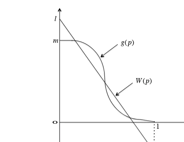
where ˆq(·) is given by (3.11). Define a functionW : [0,1]→R by
Assumption (A3) The disutility function g(p) is monotonically decreas-ing inp. It decreases rapidly from a high to a low value at some intermediate value ofp, namely it takes a sigmoid shape (as illustrated in Figure 2). Let
g(0) =m, with 0< m < l, and g(1) = 0.
l−
λ
qˆ(1)(l+ f)0
1 p
W(p)
g(p)
l
[image:18.612.105.401.161.390.2]m
Figure 2: The interior fixed points in the presence of social norms
The sigmoid shape of the disutility function g(·) captures the idea that aggregate behaviour can encourage both honest and dishonest behaviours at the individual level.
Proposition 3.3. Let assumptions (A1) and (A3) hold. Then the fixed points p∗ = 0 and p∗ = 1 of (3.17)are unstable.
As a direct consequence of Proposition 3.3, there exists at least one stable interior fixed point of (3.17).
Proof. Following the same procedure as in the proof of Theorem 3.1, the dynamics of the system are now governed by:
˙
pt= ˜h(pt) =ωβpt(1−pt) l−λqˆ(pt)(l+f)−g(pt)
. (3.20)
Differentiating the function ˜h with respect to p
d˜h
dp(p) =ωβ(1−2p)[l−λqˆ(p)(l+f)−g(p)]−ωβp(1−p)
λdqˆ(p)
dp (l+f) +g
0(p)
Then we evaluate this derivative at the boundary fixed point p∗ = 0 and obtain:
d˜h
dp(0) =ωβ(l−θ)>0. Therefore,p∗= 0 is an unstable fixed point.
The left-hand-side of (3.18) for interior fixed points is the function W defined in (3.19). The function W is decreasing in p, as it is simply a linear transformation of the authorities’ best-response function ˆq(·) which is increasing inp by Proposition 3.2. Consequently, the non-linearity of the disutility functiong allows for the possibility of multiple interior equilibria. Rewriting (3.18) yields
ˆ
q(p∗) = l−g(p
∗)
λ(l+f) = 1−
g(p∗) +λf−(1−λ)l λ(l+f) .
Sinceg(0) =m < l,g(1) = 0 andg(p) is decreasing, we have 0< g(p∗)< l. Together with the restriction (3.4), we have
0< g(p
∗) +λf−(1−λ)l
λ(l+f) <1,
namely, there exists an interior fixed point p∗∈(0,1) of (3.17) such that
0<qˆ(p∗)< l λ(l+f).
Therefore we have, at the boundary fixed pointp∗= 1
d˜h
dp(1) =−ωβ(l−λqˆ(1)(l+f))>0
that is p∗= 1 is an unstable fixed point.
Remark 3.3. The inclusion of social norms provides a mechanism for pos-itive feedback. When the initial rate of crime is low, the social disutility from crime is high (i.e. the social norm is strong), which encourages more individuals to behave honestly. This in turn acts to further reduce the rate of crime and strengthen the norm, and so on. Conversely, when the rate of crime is high, the social norm is weak and therefore the process acts in reverse.
To illustrate this point, we will take a specific example of the cost func-tion F and analysis how changes in the fine parameter f might affect the qualitative properties of these equilibria. Let F be of the form of (3.12) withα= 12N λ(l+f), i.e.
F(q) = 1
2N λ(l+f)q 2.
Then the best respond ˆq defined in (3.11) is
ˆ
p(p) =p, for all p∈[0,1]
and in turn the functionW in(3.19) is
W(p) =l−pλ(l+f). (3.21)
When p = 1, W(1) = l−λ(l+f) < 0 by the assumption (A1). In this example, the solutions of (3.18) are the intersection points of the linear function W(p) in (3.21) with the nonlinear disutility function g(p) with g(0) =m < l andg(1) = 0.
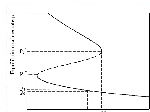
Let’s illustrate the effect of fine changes on the equilibrium with the help of Figure 3. We start with the situation that a society is initially at a low-crime equilibrium p0 when the fine is f0 (corresponding to the line W0). From this point, successive policy changes can allow the inspector to take a more lenient view on crime, namely to decrease the fine from f0 to f3 (i.e. move line W0 to line W3) without experiencing much increase in the equilibrium crime rate, i.e. the equilibrium crime rate increases slightly from p0 to p3. However, if the level of fine falls below the critical value f1∗ (i.e. the lineW0 is moved above the lineW1), there will be a drastic increase in the rate of crime (i.e. moving from p∗1 towards p∗2) as the honest norm is ’destroyed’. Moreover, undoing the policy change by increasing fine from lower than f1∗ to f0 (i.e. by moving a line above the line W1 back to W0) will not be sufficient to restore the low crime equilibriump0, since by being excessively lenient, the inspector has unwittingly fostered an undesirable social norm. Therefore the level of fine must now be increased beyondf2∗ in order to restore the population to honesty and to restore a low crime rate.
p g(p)
1 W0(p)
p1* p 2* p0p3
W3(p) W1(p)
W4(p)
(1−λ)l−λf1 *
(1−λ)l−λf2*
(1−λ)l−λf0
(1−λ)l−λf3
l
m
[image:21.612.79.425.92.400.2]0
Figure 3: Fine and equilibria
Remark 3.4. The multiple projection of the equilibrium curve on the axis of the basic parameter of the model is a general phenomenon in real life. For example, in economics Bowles [21] examined market’s instabilities of equi-librium prices. In biology, one observes the situations when small changes in drug consumptions can lead to basically irreversible changes in equilibrium states of an organism, see e.g. [35, 36].
3.3 Forward-looking inspectors
law-f0
f1* f3 f2*
p2*
p1*
p0 p3
E
qui
li
bri
um
c
ri
m
e ra
te
p
[image:22.612.127.379.93.281.2]Fine f
Figure 4: Bifurcation diagram
enforcement whilst taking into account the effect that this choice will have on future crime rates.
This can be analysed formally by replacing the static maximisation prob-lem for the inspector as described in (3.10) with an optimal control probprob-lem. Rather than optimising at each timet, the inspector now chooses an entire trajectory of the law enforcement variable {q.}={qt, t ≥0} so as to
’con-trol’ the crime ratesptvia the replicator equation (3.9). In the terminology
of optimal control problems,qtis referred to as thecontrol variableandptas
thestate variable. The objective of the inspector is to choose the trajectory
{q.} (i.e. a policy of law enforcement) that maximises the total discounted payoffs with an infinite planning horizon and a discount rateδ >0. In this subsection, social norms do not play a role in the game.
Formally, the inspector solves the following optimal control problem
max
{q.}
Z ∞
0
e−δt −F(qt) +N ptλqtf−N pt(1−λqt)l
dt
subject to ˙
pt=ωβpt(1−pt)(l−λqt(l+f)) :=P(pt, qt) (3.22)
with an initial value p0 ∈ [0,1]. The Hamiltonian function of this optimal control problemH : [0,1]×[0,1]×[0,∞)×R→Ris written as:
where µ is the dynamic Lagrange multiplier. By the Maximum Principle, the first order conditions are:
∂H
∂q(pt, qt, t, µt) =
e−δt −F0(qt) +N ptλ(l+f)
−µtωβpt(1−pt)λ(l+f) = 0 (3.23)
and
∂H
∂p(pt, qt, t, µt) =
e−δtN(λqtf−(1−λqt)l) +µtωβ(1−2pt)(l−λqt(l+f)) =−µ˙t. (3.24)
Next, we will manipulate (3.23) and (3.24) to eliminateµand ˙µand get an evolution equation forqt. Differentiating (3.23) with respect to tyields
−δe−δt −F0(qt) +N ptλ(l+f)
+e−δt −F00(qt) ˙qt+Np˙tλ(l+f)
−µ˙tωβpt(1−pt)λ(l+f)−µtωβ(1−2pt) ˙ptλ(l+f) = 0.
(3.25)
Then we solve for ˙µt from (3.24) and plug it into (3.25). Together with the
dynamics ˙pt in (3.22), the terms which contain µt are cancelled. Then we
get
−δ −F0(qt) +N ptλ(l+f)
−F00(qt) ˙qt= 0.
Hence, we derive the following equation for the evolution ofqt
˙ qt=
δ F0(qt)−N ptλ(l+f)
F00(q
t)
:=Q(pt, qt). (3.26)
Equations (3.22) and (3.26) constitute a pair of first-order differential equa-tions, which describe the optimal trajectories forpt and qt.
Theorem 3.2. Let assumptions (A1) and (A2) hold. Then,
(i) there exists only one interior fixed point(p∗, q∗)of the equations (3.22)
and (3.26) such that
(p∗, q∗) = F
0( l
λ(l+f))
N λ(l+f), l λ(l+f)
!
(3.27)
Proof. The fixed points of the equations (3.22) and (3.26) can be found by examine the nullclines, that is the sets of points at which both ˙pt and ˙qt
equal zero. In other words, any fixed point (p∗, q∗) satisfies that
P[p∗, q∗] =Q[p∗, q∗] = 0.
Specifically, letP[p∗, q∗] = 0 together with assumption(A1), we get
p∗ = 0, p∗ = 1 and p∗ ∈(0,1) such that q∗[p∗] = l
λ(l+f) ∈(0,1).
LetQ(p∗, q∗) = 0 we get
p∗ = F
0(q∗)
N λ(l+f) ∈(0,1) withq
∗ ∈(0,1)
since by assumption (A2), for anyp ∈(0,1), 0 < F0(λ(l+lf)) < N λ(l+f). Therefore, there exists an unique fixed point of the system equations (3.22) and (3.26), and the fixed point is at
(p∗, q∗) = F
0( l
λ(l+f))
N λ(l+f), l λ(l+f)
!
.
(ii) The stability of this fixed point can be analysed by examine the signs of the eigenvalues of the linearised system of differential equations (3.22) and (3.26) (c.f. [60]).
Linearising the system about the fixed point (p∗, q∗) (3.27) gives:
˙ pt ˙ qt =A
pt−p∗
qt−q∗
whereA is a 2×2 Jacobian matrix at the fixed point (p∗, q∗), i.e.
A= "∂P ∂p ∂P ∂q ∂Q ∂p ∂Q ∂q #
(p∗,q∗) =
"
0 −ωβp∗(1−p∗)λ(l+f)
−δN λF00((lq+∗)f) δ.
#
The determinant ofA is
det(A) =−ωβp∗(1−p∗)λ(l+f)δN λ(l+f) F00(q∗) <0
Remark 3.5. In this work we concentrate on the case with strictly convex cost functionF(q). In the case where the equilibrium costs are locally concave (i.e. F00(q∗) < 0), it is possible to show that the eigenvalues of the system are complex, with a positive real component. Therefore the interior state is a spiral node; all nearby trajectories spiral away from the steady-state. In this case, the precise optimal control is difficult to characterise in general terms, and depends on whether there are any additional steady-states at the boundaries which, providing they exist, will always be saddle points. However at the very least, we can conclude that the spiral nature of the interior equilibrium implies cycles in crime and law enforcement. These occur because the concave shape of the inspector’s cost function encourages ’extreme’ levels of law enforcement. That is, the inspector hardly enforces at all when crime is low as the average cost of enforcement is high. Conversely, enforcement is relatively strict when crime is high as the average cost of enforcement is relatively low. As a result, the inspector successively under and over-compensate. Meanwhile, the instability of these cycles stems from the fact that inspector discounts the future, therefore the optimal control allows crime to get out of hand in the long run.
4
Inspection with continuous strategy spaces
In the previous sections, we assume that individuals can only make a bi-nary choice between Violate and Comply. However, in many applications individuals may be able to choose the extent of their criminal activity. For example, Kolokotsov and Malafeyev [42] analysed the case of a one-shot game between a tax authority and a single individual who can choose the amount of tax to conceal from the authority.In this section we will extend analysis in [42] on inspection of a single individual by deriving the entire class of mixed strategy equilibria in this game. Then we will proceed to show that this class of equilibria also applies to games of population inspection.
4.1 Inspection of a single individual
An inspection game of a single individual with a continuous strategy space has similar structure to the canonical game in a general form specified in Section 2 (Table 2), except that:
2. we assume that the fine levied by the inspector is proportional to the severity of the individual’s crime, i.e. f =σl withσ ∈(0,1).
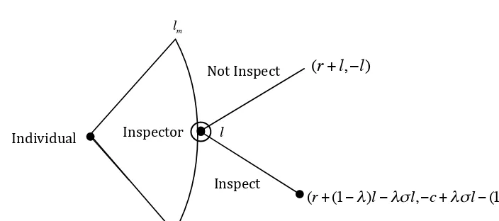
[image:26.612.77.429.210.366.2]It is worth stressing that, in this subsection we keep the assumption that the inspector chooses from the binary strategy space{Inspect, Not Inspect}. The payoffs to the inspector and the individual in the inspection game with continuous strategy space is summarised by the extensive form game in Figure 5.
Individual Inspector
Inspect Not Inspect
lm
0
(r+l,−l)
(r+(1−λ)l−λσl,−c+λσl−(1−λ)l) l
Figure 5: A single-individual inspection game with a continuous strat-egy space
In order to ensure that this game does not degenerate into dominant strategies, we impose the following regulatory conditions on the payoffs:
Assumption (A4) lm >
c
λ(σ+ 1) and λ > 1 σ+ 1.
The first inequality in assumption(A4) states that the inspector would prefer to play Inspect when the individual chooses the maximum level of crime. The second inequality in assumption(A4)states that the individual would not wish to choose to commit any level of crime when the inspector is inspecting (otherwise maximum crime is always worthwhile).
Proposition 4.1. Let assumption (A4) hold. In the inspection game with a continuous strategy space [0, lm], where lm > 0 is given, the equilibrium
state is that the individual may play any randomisation over his strategy space provided that the expected level of crime isl∗ and the inspector inspects with the probabilityq∗, with
l∗= c
λ(σ+ 1) and q
∗= 1
λ(σ+ 1).
Proof. Suppose for any probability of inspectionq ∈[0,1], the individual will only randomise over two arbitrary pure strategies, l1, l2 ∈ [0, lm] providing
that these two pure strategies yield the same expected payoff (otherwise he would want to assign full probability to the strategy yielding the higher payoff). By using the payoff table (Figure 5), we get
q[r+ (1−λ)l1−λσl1] + (1−q)[r+l1] =q[r+ (1−λ)l2−λσl2] + (1−q)[r+l2].
(4.1)
Solving equation for (4.1) gives us the equilibrium probability of inspection
q∗ = 1
λ(σ+ 1), (4.2)
which is independent of l1 and l2. This means, when the inspector plays the mixed strategy q∗ given by (4.2), the individual is in fact willing to randomise over all of his pure strategiesl∈[0, lm].
Suppose the individual’s randomisation is given by some arbitrary prob-ability density functionφ(·). Then, in order for the inspector to randomise, the expected payoff from playing Inspect must be equal to the expected payoff from playing Not Inspect, that is
Z lm 0
(−c+λσl−(1−λ)l)φ(l)dl= Z lm
0
−lφ(l)dl
which gives
Z lm 0
lφ(l)dl= c
λ(σ+ 1) :=l
∗. (4.3)
Therefore, as long as the inspector plays the mixed strategy q∗ defined in (4.2), the individual is willing to play any randomisation over all of his pure strategies l ∈ [0, lm]; Meanwhile, as long as the individual plays an
conform to these randomisations, the players’ strategies are then mutually consistent best responses.
Proposition 4.1 implies a most interesting class of mixed strategy equi-libria where the only constraint on the individual’s equilibrium behaviour is the expected level of crime. Specifically, the individual may play any mixed strategy provided that his average level of crime is λ(σc+1).
4.2 Population inspection with continuous strategy spaces
We now consider the inspector is responsible for the inspection of a large population of individuals. Specifically, we assume that there areN individ-uals, each of whom chooses a level of crimel from the continuous strategy space [0, lm]. Let Φ(·) be the probability density function of the distribution
of crime in the population. The inspector chooses the level of law enforce-ment from a continuous strategy space, i.e. q ∈ [0,1]. The cost function of law enforcement for the inspector F(·) satisfies the assumption (A1) in subsection 3.1.
Then, given a rate of enforcement q ∈ [0,1], the expected payoff for an individual from choosing the level of crimel∈[0, lm] is
E[UI(l, q)] =r+ (1−λq)l−λqσl.
Meanwhile, the expected payoff for the inspector is given by:
E[UA(q,Φ(·))] =−F(q) +λqN
Z lm 0
σlΦ(l)dl−(1−λq)N
Z lm 0
lΦ(l)dl. (4.4)
Proposition 4.2. In an population inspection game, if the inspector chooses the level of law enforcement from a continuous strategy space, i.e. q∈[0,1]
and each individual chooses a level of crime from a continuous strategy space, i.e. l ∈ [0, lm], then any distribution of crime may occur in equilibrium if
the expected level of crime isL∗ and the equilibrium probability of inspection isq∗, where
L∗ = F
0(q∗)
N λ(σ+ 1) and q
∗ = 1
λ(σ+ 1).
Suppose the resulting crime probability density function is Φ(·). The best response for the inspector can be found by maximising (4.4) overq ∈[0,1]. The relevant first order condition is:
F0(q) =N λ(σ+ 1) Z lm
0
lΦ(l)dl. (4.5)
Settingq=q∗ in (4.5) yields
Z lm 0
lΦ(l)dl= F
0(q∗)
N λ(σ+ 1) :=L
∗. (4.6)
Therefore, q∗ is a best-response to Φ(·) provided that the average level of crime isL∗ in (4.6). Meanwhile, any distribution Φ(·) with the average level of crimeL∗ in (4.6) is a best-response to the level of law enforcement isq∗. Therefore (L∗, q∗) constitutes a mixed strategy Nash equilibrium.
This class of equilibria is particularly interesting for population-level inspection games, as it implies that populations with similar levels of law-enforcement can exhibit markedly different patterns of crime. In some pop-ulations, crime may be the preserve of a minority of relatively serious of-fenders, whereas in others, moderate levels of crime may be widespread. In terms of law enforcement, only the average level of crime matters.
References
[1] J. Alm, M. McKee (2004). Tax compliance as a coordination game. Journal of Economic Behaviour and Organization, 54, 297-312.
[2] S. Alpern, A. Morton, K. Papadaki (2011). Patrolling games. Operations Re-search, 59, 1246-1257.
[3] U. Anderson, R.A. Young (1988). Internal audit planning in an interactive environment. Auditing: A Journal of Practice and Theory, 8(1), 23-42.
[4] L. Andreozzi (2010). Inspection games with long-run inspectors. European Journal of Applied Mathematics, 21(4-5), 441-458.
[5] L. Andreozzi (2004). Rewarding policemen increases crime: another surprising result from the inspection game. Public Choice, 121(1), 69-82.
[6] R. Avenhaus (1994). Decision theoretic analysis of pollutant emission moni-toring procedures. Annals of Operations Research, 54(1), 23-38.
[7] R. Avenhaus (1986). Safeguards Systems Analysis. Plenum, New York.
[9] R. Avenhaus, M.J. Canty (2005). Playing for time: a sequential inspection game. European Journal of Operational Research, 167(2), 475-492.
[10] R. Avenhaus, J.M. Canty (2009). Inspection games, in: R.A. Meyers (Ed.), The Encyclopedia of Complexity and Systems Science, Vol. 5, Springer, New York, 4855-4868.
[11] R. Avenhaus, J.M. Canty (2011). Deterrence, technology and the sensible distribution of arms control verification resources. Naval Research Logistics, 58(3), 295-303.
[12] R. Avenhaus, M. D. Canty, D. M. Kilgour, B. von Stengel, S. Zamir (1996). Inspection games in arms control. European Journal of Operational research, 90(3), 383-394.
[13] R. Avenhaus, D. Kilgour (2004). Efficient distributions of arm-control inspec-tion effort. Naval Research Logistics, 51(1), 127.
[14] R. Avenhaus, B. von Stengel (1991). Non-zero-sum Dresher inspection games. Contribution to the 16th Symposium Operation s Research, Trier, Germany, September.
[15] R. Avenhaus, B. von Stengel (1991). Current research in data verification. Con-tribution to the IMACS International Workshop on Decision Support Systems and Qualitative Reasoning, Toulouse, France, March 1315.
[16] R. Avenhaus, B. Von Stengel, S. Zamir (2002). Inspection games. In: R. Au-mann, S. Hart (Eds.) Handbook of Game Theory with Economic Applications, Vol. 3 North-Holland, Amsterdam, 1947- 1987.
[17] V. Baston, F. Bostock (1991). A generalized inspection game. Naval Research Logistics, 38(2), 171-182.
[18] G.S. Becker (1968). Crime and punishment: an economic approach. Journal of Political Economy, 76, 169.
[19] K. Borch (1982). Insuring and auditing the auditor. In: Games, Economic Dy-namics, Time Series Analysis, eds. M. Deistler, E. F¨urst, and G. Schw¨odiauer. Physica-Verlag, Vienna, 117-126.
[20] K. Borch (1990). Economics of Insurance. Advanced Textbooks in economics, 29, North-Holland, Amsterdam, 350-362.
[21] S. Bowles. Microeconomics. Behavior, Institutions and Evolution. Russell Sage Foundation, 2004.
[22] M.J. Canty, D. Rothenstein, R. Avenhaus (2001). Timely inspection and de-terrence. European Journal of Operational Research, 131(1), 208-223.
[24] Y. Deutsch, B. Golany, U.G. Rothblum (2011). Determining all Nash equilibria in a (bi-linear) inspection game. European Journal of Operational Research, 215(2), 422-430.
[25] H. Diamond (1982). Minimax policies for unobservable inspections. Mathe-matics of Operations Research, 7(1), 139-153.
[26] M. Dresher (1962). A sampling inspection problem in arms control agreements: a game-theoretic analysis, memorandum RM-2972-ARPA, The RAND corpo-ration, Santa Monica, California.
[27] G. Fandel, J. Trockel (2008). Stockkeeping and controlling under game theo-retic aspects. Advanced Management Science (ICAMS), 1, 563-567.
[28] G. Fandel, J. Trockel (2008). Efficient storage under the aspect of conflict-ing priorities between stockkeepconflict-ing and controllconflict-ing. In Fifteenth International Working Seminar on Production Economics, Pre-Prints, Vol. 3, Innsbruck, 87-100.
[29] G. Fandel, J. Trockel (2011). Optimal lot sizing in a non-cooperative material manager controller game. International Journal of Production economics, 133 (1), 256-261.
[30] G. Fandel, J. Trockel (2012). A three-person inspection game in production economics. working paper.
[31] T. Ferguson, C. Melolidakis (1998). On the inspection game. Naval Research Logistics, 45, 327334
[32] J. H. Fowler (2005). Altruistic punishment and the origin of cooperation. Pro-ceedings of the National Academy of Sciences of the United States of America. 102(19), 7047-7049.
[33] A. Garnaev (1994). A remark on the customs and smuggler game. Naval Re-search Logistics, 41(2), 287-293.
[34] G. Gianini, T.R. Mayer, D. Coquil, H. Kosch, L. Brunie (2012). Inspection games for selfish network environments, working paper, University of Passau.
[35] A.N. Gorban, L.I. Pokidysheva,E,V. Smirnova, T.A. Tyukina (2011). Law of the Minimum Paradoxes. Bulletin of Mathematical Biology, 73(9), 2013-2044.
[36] A.N. Gorban, E.V. Smirnova, T.A. Tyukina (2010). Correlations, risk and cri-sis: From physiology to finance. Physica A Statistical and Theoretical Physics, 389(16), 3193-3217.
[37] J. Greenberg (1984). Avoiding tax avoidance: a (repeated) game-theoretic approach. Journal of Economic Theory, 32(1), 1-13.
[39] R. Hohzaki (2007). An inspection game with multiple inspectees. European Journal of Operational Research, 178(13), 894-906.
[40] C.C. Hsieh, Y.T. Liu( 2010). Quality investment and inspection policy in a supplier-manufacturer supply chain. European Journal of Operational Re-search, 202(3), 717-729.
[41] A. Klages (1968). Spieltheorie und Wirtschaftspr¨ufung: Anwendung spielthe-oretischerModelle in der Wirtschaftspr¨ufung. Schriften des Europa-Kollegs Hamburg, Vol. 6, Ludwig Appel Verlag, Hamburg.
[42] V.N. Kolokoltsov, O.A. Malafeyev (2010). Understanding Game Theory: Intro-duction to the analysis of many agent systems of competition and cooperation. London, UK: World Scientific.
[43] H.W. Kuhn (1963). Recursive inspection games. In: Applications of Statisti-cal Methodology to Arms Control and Disarmament, eds. F.J. Anscombe et al., Final report to the U.S. Arms Control and Disarmament Agency under contract No. ACDA/ST-3 by Mathematica, Inc., Princeton, New Jersey , Part III, pp. 169-181.
[44] A. Lindbeck, S. Nyberg, J.W. Weibull (1999). Social norms and economic incentives in the welfare state. Quarterly Journal of Economics, 114(1), 1-35.
[45] R. L´opez-P´erez (2006). Introduction social norms in game theory. Working paper, University of Zurich, 292.
[46] M. Maschler (1966). A price leadership method for solving the inspection’s non-constant-sum game, Naval Research Logistics Quarterly, 13, 11-13.
[47] W. M. McEneaney, R. Singh (2006). Robustness against Deception. In: Ad-versarial Reasoning: Computational Approaches to Reading the Opponents Mind, Eds, A. Kott, W. M. McEneaney, Chapter 2.4. CRC Press.
[48] R. Pradiptyo (2006).”Does Punishment Matter? A Refinement of the Inspec-tion Game,” German Working Papers in Law and Economics 2006-1-1142, Berkeley Electronic Press.
[49] H. Rauhut (2009). Higher punishment, less control? Experimental evidence on the inspection game. Rationality and Society, 21(3), 359-392.
[50] J.F. Reinganum, L.L. Wilde (1985). Income tax compliance in a principal-agent framework. Journal of Public Economics, 26(1), 1-18.
[51] J.F. Reinganum, L. L. Wilde (1986). Equilibrium verification and reporting policies in a model of tax compliance. International Economic Review, 27(3), 739-760.
[53] D. Rothenstein, S. Zamir (2002). Imperfect inspection games over time. Annals of Operations Research, 109, 175-192.
[54] A. Rubinstein (1979). An optimal conviction policy for offenses that may have been committed by accident. In: Applied Game Theory, eds. S. J. Brams, A. Schotter, and G. Schw¨odiauer, Physica-Verlag, W¨urzburg, 373-389.
[55] W. H. Ruckle (1992). The upper risk of an inspection agreement. Operations Research, 40(5), 877-884.
[56] G.S. Russell (1990). Game models for structuring monitoring and enforcement systems. Natural Resource Modeling, 4(2), 143-173.
[57] M. Sakaguchi (1994). A sequential game of multi-opportunity infiltration. Mathematica Janonica, 39 ,157-166.
[58] H. Schleicher (1971). A recursive game for detecting tax law violations. Economies et Soci´et´es, 5, 1421-1440.
[59] K. Sigmund, C. Hauert, A. Traulsen , H. De Silva (2011). Social control and the social contract: The emergence of sanctioning systems for collective action. Dynamic Games and Applications, 1(1), 149-171.
[60] S.H. Strogatz (1994). Nonlinear dynamics and chaos: with applications to physics, biology, chemistry and engineering. Cambridge, MA: Westview Press.
[61] C.S. Tapiero, K.Kogan (2007). Risk and quality control in a supply chain: Competitive and collaborative approaches. Journal of The Operational Re-search Society, 58, 1440-1448.
[62] P. Taylor, L. Jonker(1978). Evolutionary Stable Strategies and Game Dynam-ics, Mathematical Biosciences, 40(2), 145-156.
[63] M. Thomas, Y. Nisgav (1976). An infiltration game with time dependent pay-off. Naval Research Logistics Quarterly, 23(2), 297-302.
[64] G. Tsebelis (1989). The abuse of probability in political analysis: the robinson crusoe fallacy. The American Political Science Review, 83(1), 77-91.
[65] B. von Stengel (1991). Recursive inspection games, IASFOR-Bericht S-9106.
[66] A. Washburn, K. Wood (1995). 2-person zero-sum games for network interdic-tion. Operations Research, 43(2), 243-251.
[67] F. Weissing, E. Ostrom (1991). Irrigation institutions and the games irrigators play: rule enforcement without guards. In: Game Equilibrium Models II, eds. R. Selten, Springer, Berlin, 188-262.