City, University of London Institutional Repository
Citation
: Benetos, E. and Kotropoulos, C. (2010). Non-Negative Tensor Factorization
Applied to Music Genre Classification. IEEE Transactions on Audio, Speech & Language
Processing, 18(8), pp. 1955-1967. doi: 10.1109/TASL.2010.2040784
This is the unspecified version of the paper.
This version of the publication may differ from the final published
version.
Permanent repository link:
http://openaccess.city.ac.uk/2048/
Link to published version
: http://dx.doi.org/10.1109/TASL.2010.2040784
Copyright and reuse:
City Research Online aims to make research
outputs of City, University of London available to a wider audience.
Copyright and Moral Rights remain with the author(s) and/or copyright
holders. URLs from City Research Online may be freely distributed and
linked to.
IEEE TRANSACTIONS ON AUDIO, SPEECH, AND LANGUAGE PROCESSING 1
Non-negative Tensor Factorization Applied to Music
Genre Classification
Emmanouil Benetos and Constantine Kotropoulos, Senior Member, IEEE
Abstract—Music genre classification techniques are typically
applied to the data matrix whose columns are the feature vectors extracted from music recordings. In this paper, a feature vector is extracted using a texture window of one sec, which enables the representation of any 30 sec long music recording as a time sequence of feature vectors, thus yielding a feature matrix. Consequently, by stacking the feature matrices associated to any dataset recordings, a tensor is created, a fact which necessitates studying music genre classification using tensors. First, a novel algorithm for non-negative tensor factorization (NTF) is derived that extends the non-negative matrix factorization. Several vari-ants of the NTF algorithm emerge by employing different cost functions from the class of Bregman divergences. Second, a novel supervised NTF classifier is proposed, which trains a basis for each class separately and employs basis orthogonalization. A variety of spectral, temporal, perceptual, energy, and pitch descriptors is extracted from 1000 recordings of the GTZAN dataset, which are distributed across 10 genre classes. The NTF classifier performance is compared against that of the multilayer perceptron and the support vector machines by applying a stratified 10-fold cross validation. A genre classification accuracy of 78.9% is reported for the NTF classifier demonstrating the superiority of the aforementioned multilinear classifier over several data matrix-based state-of-the-art classifiers.
Index Terms—Non-negative tensor factorization, Bregman
di-vergences, Music genre classification.
I. INTRODUCTION
C
URRENT advances in multimedia data management and retrieval have enabled the creation, distribution, and availability of vast amounts of music data including new content as well as digitized one from analog archives. Aided by the growth of the internet, these databases have become highly popular for personal as well as commercial use (e.g. online music retailers or digital libraries). Accordingly, the demand for tools to analyze and retrieve music content has emerged, leading to flourishing music information retrieval (MIR) research.Music genres are the most popular music content descrip-tors, since they are employed by both the users and the music industry [1]. One may argue that the genres sum-marize music recordings based on some common perceptual characteristics [2]. However, music genres have not yet been precisely defined, because they are primarily determined by users’ taste and may be culturally dependent. Not to mention
E. Benetos is currently with the Dept. of Electronic Engineering, Queen Mary University of London, Mile End Road, London, E1 4NS, United King-dom. He was with the Dept. of Informatics, Aristotle University of Thessa-loniki, Box 451, Thessaloniki 54124, Greece. C. Kotropoulos is with the Dept. of Informatics, Aristotle University of Thessaloniki, Box 451, Thessaloniki 54124, Greece. E-mail: [email protected], [email protected]
that more than one music genres may be associated with a certain recording. Accordingly, the creation of a universal genre taxonomy remains still infeasible. Automatic genre clas-sification techniques classify recordings into distinguishable genres by extracting relevant features and employing pattern recognition algorithms [3]. The accuracy of such genre clas-sification techniques often exceeds that reported for humans with moderate music training [4]. However, the research on automatic genre classification appears to have reached a local maximum recently due to the lack of carefully annotated music corpora with ground truth [5].
Most genre classification approaches represent each music recording by a feature vector and consequently employ pattern recognition algorithms in order to perform classification. In this paper, each recording is represented by a time sequence comprising feature vectors extracted every one sec, thus forming a feature matrix. Starting with a comprehensive set of features measuring spectral, temporal, perceptual, energy, and pitch characteristics of the recordings, feature selection is applied next by using a branch-and-bound search strategy in order to determine the subset of the most discriminative features with respect to the ratio of the inter-class dispersion over the intra-class dispersion [9] and keep the number of the features to be processed into a manageable size. By stacking the feature matrices associated to recordings, a tensor is created, which provides a more detailed representation of music characteristics. Tensors are considered as extensions of matrices or vectors [6]–[8]. A novel non-negative tensor factorization (NTF) algorithm is proposed whose roots are traced back in the non-negative matrix factorization (NMF). The algorithm is able to decompose a tensor in Kruskal format [8]. That is, to decompose a tensor into a sum of elementary rank-1 tensors. The algorithm can employ sev-eral cost functions, which belong to the class of Bregman divergences [10]. The Bregman divergences have previously been used to solve the non-negative matrix approximation problem [11]. Details on the derivation of the tensor element update equations are provided and the computational cost of the algorithm is estimated. In addition, a novel supervised classifier based on the NTF is proposed, which trains a basis for each class separately and employs basis orthogonalization. The proposed classifier extends a similar classifier that was based on the NMF [34]. Preliminary results for music genre classification using the NTF classifier with the Frobenius norm as cost function were reported in [33]. Here, starting from a larger feature set than that used in [33], results are reported on extended experiments performed on the GTZAN database, which contains 1000 music recordings covering
this material for advertising or promotional purposes, creating new collective works for resale or redistribution to servers or lists, or reuse of any copyrighted components of this work in other works.
10 music genre classes [12]. Several variants of the NTF classifier employing different feature subset sizes are tested and their music genre classification accuracy is measured using a stratified 10-fold cross-validation. For comparison purposes, support vector machines and multilayer perceptrons are also tested on the same database. In addition, experiments are performed using the features extracted by the MARSYAS platform [39]. An average genre classification accuracy of 78.9% with standard deviation equal to 2.6% is reported for the NTF classifier, when the Frobenius norm is utilized with a subset of 80 features. The aforementioned accuracy places the proposed NTF classifier within the most performing state-of-the-art genre classification methods. The superiority of the NTF classifier against the state-of-the-art data matrix-based classifiers is also demonstrated. Such results motivate further research using tensorial representations into audio processing applications.
The outline of the paper is as follows. Related work on automatic music genre classification is discussed in Section II. Section III details the proposed NTF method and establishes links with the NMF as well as other methods proposed for the NTF. In this section, a supervised classifier based on the proposed NTF is also described. Section IV briefly presents the dataset used, the feature set employed in the experiments, and thoroughly assesses the music genre classification accuracy of the proposed NTF classifier against that of state-of-the-art classifiers. Conclusions are drawn and future directions are indicated in Section V.
II. RELATEDWORK
Several benchmark datasets have been collected making the performance of the various music genre classification approaches comparable. Such benchmark datasets are listed in Table I along with the best accuracy reported for state-of-the-art classifiers in chronological order. The GTZAN dataset was introduced by Tzanetakis and Cook [12]. It contains 1000 audio recordings split into 10 genre classes. The parameters of a Gaussian mixture model (GMM) classifier were estimated by the iterative expectation-maximization (EM) algorithm in [12]. A 61% correct classification was reported for timbre, rhythmic, and pitch features. The same dataset was used by Li et al. who employed support vector machines (SVMs) and linear discriminant analysis (LDA) for classification [13]. The Daubechies wavelet coefficient histograms were used as features and the reported classification accuracy of the SVM classifier reached 78.5%. Lidy and Rauber employed a pairwise SVM classifier applied to the GTZAN dataset [3]. The extracted features include rhythm patterns, a statistical spectrum descriptor, and rhythm histogram features. The re-ported best classification accuracy was 74.9%. Bergstra et al. tested the mel-frequency cepstral coefficients (MFCCs), the fast Fourier Transform coefficients, the linear prediction coefficients (LPCs), and the zero-crossing rate (ZCR) on the GTZAN dataset [14] and reported a classification accuracy reaching 82.5% for the ADABOOST meta-classifier. It should be noted, however, that the classification accuracy in [14] was measured without cross-validation. Holzapfel and Stylianou
TABLE I
CLASSIFICATION ACCURACY(IN%)OF SEVERAL MUSIC GENRE CLASSIFIERS IN CHRONOLOGICAL ORDER. THE HIGHEST ACCURACY IS
SHOWN IN BOLDFACE.
Reference Dataset Classifier Best Accuracy
[12] GTZAN GMM 61.0
[13] GTZAN SVM - LDA 78.5
[3] GTZAN SVM 74.9
[14] GTZAN ADABOOST 82.5
[15] GTZAN GMM 74.0
[17] MIREX 2004 NN - GMM 82.3
[3] MIREX 2004 SVM 70.4
[15] MIREX 2004 GMM 83.5
also employed the same dataset. By utilizing a spectral basis derived by the NMF, that is fed to a GMM classifier, they obtained a 74.0% classification accuracy [15].
Another collection used extensively is the MIREX 2004 dataset, released for the MIREX genre and rhythm classifi-cation contests [16]. The MIREX 2004 genre dataset contains 1458 recordings belonging into 6 genre classes. The best accuracy (i.e. 83.5%) was reported by Holzapfel and Stylianou [15]. Pampalk et al. used the nearest neighbor (NN) classifier with GMMs and obtained an accuracy of 82.3% [17]. In our experiments, we are confined to the GTZAN dataset, because it contains more genre classes than the MIREX 2004 one, thus being a more comprehensive dataset for genre classification.
III. NON-NEGATIVETENSORFACTORIZATION
In this section, a novel non-negative tensor factorization (NTF) technique is developed. First, the non-negative matrix factorization (NMF) is briefly discussed, because the NTF could be treated as a high-order generalization of the NMF for tensorial data. Some definitions from tensor algebra follow and the motivation for using tensors is described. Previous NTF algorithms are reviewed next and the proposed one is detailed. Contrary to previous approaches, the proposed NTF algorithm is not limited to 3rd order tensors, but can be applied tonth (n>3) order tensors. In addition, the algorithm can be
formulated using a variety of objective functions. Obviously, its use is not restricted to audio processing only. Finally, a novel supervised classifier based on NTF for 3rd order tensors is proposed, which performs separate training for each class and employs basis orthogonalization.
Throughout the paper, tensors are denoted by boldface Euler script calligraphic letters (e.g. A), matrices are denoted by
uppercase boldface letters (e.g. U), and vectors are denoted by lowercase boldface letters (e.g. u). The elements of all the aforementioned mathematical structures are denoted by lowercase letters indexed by one or more indices. For example, the elements of matrix U are denoted as u
i 1
i 2
. LetR andZ
be the sets of real and integer numbers, respectively.
A. Non-negative Matrix Factorization
Subspace analysis seeks low dimensional structures of pat-terns within high dimensional spaces. NMF is a subspace method able to obtain a parts-based representation of objects by imposing non-negative constraints. It was first introduced as positive matrix factorization by Paatero et al. [22] and was re-termed as NMF by Lee and Seung [23]. The problem addressed by the NMF is as follows. Given a non-negative real-valued data matrix V 2 R
nm +
, find the non-negative matrix factorsW2R
nk +
andH2R km +
so that
VWH= k X
i=1 w
i h
T i
, k X
i=1 w
i Æh
i (1)
where Æ stands for the outer product. Obviously,w
i are the
columns of W and h T i
are the rows of H. W contains the
basis vectors, while the column vectors of H contain the
weights needed to properly approximate the corresponding column vector of V as a linear combination of the column
vectors ofW. Usually,k is chosen so that(n+m)k<nm,
thus resulting in a compressed version of the original data matrix. To find the approximate factorization (1), a suitable objective function has to be minimized. Let V = [v
ij ℄ and WH ,Y =[y
ij
℄. In [23], the generalized Kullback-Leibler
(KL) divergence betweenV andWHwas used:
D(V jjWH)= n X
i=1 m X
j=1
v ij
log v
ij y
ij v
ij +y
ij
(2)
The minimization of (2) can be solved by using iterative multiplicative rules [23]. Frequently, additional constraints are incorporated into (2). For example, the local NMF algorithm
I 2
I3 I
1
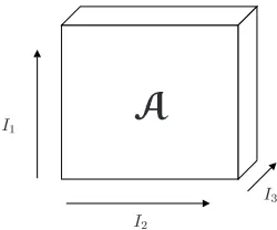
[image:4.595.380.505.101.205.2]A
Fig. 1. 3rd order real-valued tensorA2R I
1 I
2 I
3.
imposes spatial locality in the solution and consequently reveals local features in the data matrixV [24].
A more general view of the NMF is set under the so-called non-negative matrix approximation (NNMA) in [11]. In NNMA, instead of minimizing a specific objective function, the minimization of a class of objective functions, called
Bregman divergences, is proposed. The same approach will
be adopted for the derivation of the NTF in Subsection III-D.
B. Tensors and Multilinear Algebra Basics
Quantities addressed by more than two indices are often employed in signal processing applications. To describe such quantities, tensors need to be employed. In multilinear algebra, tensors are considered as high-order generalizations of matri-ces and vectors [6]–[8]. A real-valued vectora2R
I
,I 2Zis
treated as a first-order tensor. Similarly, a real-valued matrix
A 2 R I1I2
with I 1
;I 2
2 Z is defined as a second-order
tensor. A real-valued tensorAof ordernis defined over the
vector spaceR
I1I2In
, whereI i
2Z,i=1;:::;n. Each
element of Ais addressed by nindices, i.e. a i
1 i
2 :::i
n
, where
i i
=1;2;:::;I
i. A 3rd order tensor is sketched in Figure 1.
Mode-iunfolding of the tensorAyields the matrix A (i)
2 R
IiIi
, whereI i
,I 1
I 2
I i 1
I i+1
I
n. In the following,
the operations on tensors are expressed in matricized form [8]. The symbol
i stands for the
i-mode product between a
tensor and a matrix [6]. It can be computed via the matrix mul-tiplication B(i)
=UA
(i) followed by re-tensorization to undo
the mode-i unfolding for i = 1;2;:::;n. For example, the
2-mode product between the 3rd order tensorA2R I
1 I
2 I
3
and the matrix U 2 R I
2 J
yields the 3rd order tensor
B = A 2
U 2 R I
1 JI
3. The inner product of two nth
order tensors A andB is denoted as <A;B>. The norm
of tensorA is defined asjjAjj= p
<A;A>.
Ann-order tensorAhas rank1, when it can be decomposed
as the outer product ofnvectors u (1)
;u (2)
;:::, u (n)
, i.e.
A=u (1)
Æu (2)
Æ:::Æu (n)
: (3)
That is, each element of the tensor in (3) is given by
a i
1 i
2 :::i
n = u
(1) i
1 u
(2) i
2 ::: u
(n) i
n
for all i `
= 1;2;:::;I ` and ` = 1;2;:::;n. The rank of an arbitrary n-order tensor A
is the minimal number of rank-1tensors that yield A when
linearly combined.
Khatri-Rao product denoted by , whose definitions can be
found elsewhere, e.g. [8].
C. Motivation for Using Tensors and the Proposed Non-negative Tensor Factorization
The NMF has been used extensively in signal processing yielding promising results in the past years. A list of the numerous NMF applications can be found in [11]. However, the NMF as any other subspace method deals only with vectorized data. By vectorizing a typical 3rd order tensor stemming from 900 training recordings, which are represented by 30 feature vectors of 34 dimensions each, one obtains 900 vectors of 1020 dimensions. Many pattern classifiers cannot cope with the aforementioned dimensionality given the small number of training samples. In addition, handling such high-dimensional samples is computationally expensive. For example, eigen-analysis or singular value decomposition cannot be easily performed. Despite implementation issues, it is well understood that vectorization breaks the natural structure and correlation in the original data. Thus, in order to preserve the natural data structure and correlation, dimen-sionality reduction operating directly on tensors rather than vectors is desirable. The concept of low-rank decomposition of high-order signal representations is addressed in [6], [25], where several algorithms are reviewed. Thus, a high-order generalization of the NMF could be of great importance in the analysis of such high-order signal/pattern representations. Some NMF generalizations have been proposed mostly for 3rd order tensors in face detection or recognition applications. In 2005, Shashua and Hazan proposed a generalization of the NMF fornth order tensors [26]. The problem was formulated
as the decomposition of a tensor into a sum ofkrank-1 tensors
using the Frobenius norm as distance. Multiplicative update rules were employed and an application to sparse image coding was discussed. Hazan et al. extended the previous work by employing the KL divergence (also known as relative entropy) as distance [27].
In 2006, Boutsidis et al. introduced an algorithm for 3rd order tensor decomposition called projected alternating least squares with initialization and regularization (PALSIR) [28]. This algorithm also employed the Frobenius norm as distance and alternating least squares was used to derive the decompo-sition. Experiments were performed on eye image databases for biometric iris recognition applications. Heiler and Schn ¨orr proposed a generalization of the sparse NMF algorithm for 3rd order tensors applied to face detection [29]. The Frobenius norm was used as distance in this case, too. The algorithm was termed as sparsity-constrained NTF, because a sparsity maximization algorithm was employed.
In 2007, Cichocki proposed algorithms for 3rd order NTF using alpha and beta divergences [30]. These algorithms employed alternating interior-point gradient and fixed point alternating least squares techniques incorporating sparsity constraints into the decomposition. The just described NTF method was incorporated into multilayer networks in order to improve the performance of multi-way blind source separation in EEG [31]. It should be noted that this model cannot be
generalized to higher order tensors nor can degenerate to the NMF model for 2nd order tensors.
In this paper, we would like to derive a generic unified NTF algorithm, which can handlenth order tensors and can
degenerate to the NMF, whenn=2.
D. Proposed NTF Algorithm
Having set our objectives, we decided to build upon the model proposed by Shashua and Hazan [26], which can be extended to nth order tensors and degenerates to the NMF,
when n = 2. A preliminary version of the algorithm was
first introduced in [33], which was also the basis for the Discriminant NTF algorithm in [32]. We resort to the Bregman divergences in order to offer a unified factorization framework, which includes as special cases the Frobenius norm, the KL-divergence, and the Itakura-Saito (IS) distance. The Bregman divergences, proposed by Bregman in 1967 [10], are defined as
D
(x;y)=(x) (y) 0
(y)(x y); (4)
where(x)is a strictly convex function defined on a convex
set S R and 0
(y) denotes the first derivative of ()
evaluated at y. By definition, the Bregman divergences are
non-negative [11] and can be extended to tensors. Let us consider the nth order tensors X ;Y 2 R
I 1
I 2
I n. The
following identity holds:
D
(X ;Y)= I
1 X
i1=1 I
2 X
i2=1
I n X
in=1 D
(x
i 1
i 2
:::i n
; y i
1 i
2 :::i
n ): (5)
For(x)= 1 2 x
2
,D
(x;y)corresponds to the Frobenius norm.
For(x)=xlog(x), the Bregman divergence coincides with
the KL divergence, whereas for(x)= log(x), the resulting
D
(x;y)is recognized to be the Itakura-Saito (IS) distance.
Therefore, our goal is to decompose a tensor V 2
R
I1I2In +
into a sum ofk rank-1 tensors:
V= k X
j=1 u
(1) j
Æu (2) j
ÆÆu (n) j
(6)
where u (i) j
2 R Ii + and
j = 1;2;:::;k. Let U (i)
,
[u (i) 1
ju (i) 2
j:::ju (i) k
℄,i=1;2;:::;n. ObviouslyU (i)
2R Iik +
. Let us introduce the compact notation
K
i U,U
(n)
U (i+1)
U (i 1)
U (1)
: (7)
In matricized form, the factorization (6) can be written as:
V (i)
, U
(i) |{z} W
(i)
U (n)
U (i+1)
U (i 1)
U (1)
| {z }
H (i)
T
= U
(i)
K
i U
T
: (8)
From the inspection of (8), one may readily see that the NMF results if W =W
(1) =U
(1)
and H =[H (1)
℄ T
=[U (2)
℄ T
. Let
X
%i ,
I1 X
% =1 I2 X
% =1
Ii 1 X
% =1 Ii+1 X
% =1
In X
% =1
The following minimization problem with Bregman diver-gences is solved
min u (i) j 0 D k X j=1 u (1) j Æu (2) j
ÆÆu (n) j
;V
(10)
by using auxiliary functions, as is analyzed in Appendix I. In particular, for the KL divergence (i.e. (x) = xlog (x)),
the following multiplicative update rule is obtained for the elements ofu
(i) j
denoted asu (i) jl : u (i) jl ~ u (i) jl exp P %i j% 1 :::% i 1 % i+1 :::% n log v % 1 :::% i 1 l% i+1 :::%n % 1 :::% i 1 l% i+1 :::% n P %i j% 1 :::% i 1 % i+1 :::% n (11) where u~
(i) jl
is the lth element of vectoru (i) j
before updating,
j =1;2;:::;k,i=1;2;:::;n,l=1;2;:::;I i, and
j%1:::%i 1%i+1:::%n =u (1) j%1 u (i 1) j%i 1 u (i+1) j%i+1 u (n) j%n (12) %1:::%i 1l%i+1:::%n = k X j 0 =1 u (1) j 0 %1 u (i 1) j 0 %i 1 u (i) j 0 l u (i+1) j 0 %i+1 u (n) j 0 %n : (13)
For (x)= 1 2 x
2
(that is, when the Frobenius norm is used), the resulting update rule is:
u (i) jl ~ u (i) jl P % i j%1:::%i 1%i+1:::%n v %1:::%i 1l%i+1:::%n P % i j%1:::%i 1%i+1:::%n %1:::%i 1l%i+1:::%n : (14) Finally, for (x) = log(x) (i.e. when the IS distance is
employed), the update rule is:
u (i) jl ~ u (i) jl P % i j% 1 :::% i 1 % i+1 :::%n % 1 ::: % i 1 l% i+1 ::: %n P % i j% 1 :::% i 1 % i+1 :::% n v % 1 :::% i 1 l% i+1 :::%n : (15)
In order to apply the aforementioned NTF algorithms to annth
order tensorV, thenmatricesU (i)
,i=1;2;:::;n, should be
initialized by random numbers between 0 and 1. The update rules (11), (14), or (15) are applied to the column vectorsu
(i) j
of matrixU (i)
,j=1;2;:::;k. The proof of convergence for
the Frobenius NTF algorithm can be found in Appendix I. The computational cost of the various NTF algorithms is derived in Appendix II.
E. Proposed 3rd Order NTF Classifier
The novel NTF classifier for 3rd order tensors discussed next was inspired by the NMF classifier proposed in [34], where a basis for each class was trained separately and the test data were projected onto an orthogonalized basis. Preliminary results using the proposed classifier for 3rd order tensors in music genre classification were reported in [33]. Let C be
the number of genre classes. The proposed 3rd order NTF classifier considers a tensor V
2R
I1I2I3
with I
1 being
the number of training recordings in class , =1;2;:::;C
(i.e. 90 for stratified 10-fold cross-validation in the GTZAN dataset), I
2 being the dimensionality of feature vectors, I
3 = 30being the number of feature vectors extracted per recording
(i.e. the number of 1 sec segments each recording is split to). The algorithm steps are as follows:
1) Decompose the training tensor for each genre V
2 R
I1I2I3
,=1;2;:::;C, i.e.
V = k X j=1 u (1) j Æu (2) j Æu (3) j : (16)
2) Determine the 1st mode of the tensor V
by unfolding [6], [8]: V (1) =U (1) U (3) U (2) T (17)
wherestands for the Khatri-Rao matrix product. Thus,
U (3) U (2) has dimensions (I 3 I 2
)k, whileV
(1)
is a matrix with dimensionsI
1 (I
3 I
2
). In the following,
we deal with the transpose of matrixV (1) , i.e. [V (1) ℄ T = U (3) U (2) [U (1) ℄ T : (18)
3) Perform QR decomposition on the basis matrixU (3) U (2) : U (3) U (2) =Q R (19) whereQ is a (I 3 I 2
)kcolumn-orthogonal matrix (i.e. Q
T
Q is the
kkidentity matrix)
1and
R is a
kk
upper triangular matrix. Store matrices Q and H = R [U (1) ℄ T
. It is worth noting that the Gram-Schmidt orthogonalization does not affect the non-negativity of the basis matrix. It is used to calculate correctly theL
2
norms in a non-orthogonal basis. 4) For testing, the feature matrix V
t of dimensions I
2 I
3 is considered. The feature matrix is arranged to a
column vectorv
t of dimensions I
2 I
3 by concatenating
its columns. The column vectorv
t is projected onto the
subspaces defined by the basis matrices of the classes:
h t =Q T v t (20)
and has length k.
5) LetCSM tm
()be the cosine similarity measure (CSM)
between h t and
h m,
m = 1;2;:::;I
1 (i.e. the mth
column of matrixH ): CSM tm ()= h T t h m jjh t jjjjh m jj : (21)
Let CSM t[m℄
()denote themth largest element in the
set fCSM tm
(); m = 1;2;:::;I 1
g. The decision
taken by the classifier is based on
$ t ()= K X m=1 CSM t[m℄ () (22)
where K I 1 (e.g.
K =3). The class label of the
test pattern v
t is determined by the maximum among $
t
(), i.e.: ^ t = argmax =1;2;:::;C f$ t ()g: (23)
A block diagram of the testing procedure of the proposed supervised NTF classifier is sketched in Figure 2.
1Obviously,
QQ T
v t
. . .
h 2t
h Ct
.
. .
.
. .
Q T 1
Q T 2
Q T C
h 1t
H 1
H 2
H C
arg max
h t
=Q T v
t
$ t
(C) $
t (1)
$ t
[image:7.595.311.560.111.312.2](2)
Fig. 2. The proposed supervised NTF classifier.
IV. EXPERIMENTALRESULTS
In this Section, music genre classification experiments are discussed. In subsection IV-A, the employed dataset is de-scribed. The feature extraction is detailed in subsection IV-B, while the feature selection method is discussed in subsection IV-C. Finally, the accuracy using the various classifiers is reported in subsection IV-D.
A. Dataset
The GTZAN database was employed for genre classification experiments. The database contains 1000 audio recordings distributed across 10 music genres [12], namely: Classical, Country, Disco, HipHop, Jazz, Rock, Blues, Reggae, Pop, and Metal. 100 recordings are collected for each genre. All recordings are mono channel, are sampled at 22050 Hz rate, and have a duration of approximately 30 sec. Each recording is separated into 30 segments (i.e. texture windows) of 1 sec duration. Such a texture window has commonly been used in genre classification experiments, because it increases the classification accuracy compared to direct analysis frames [2], [12], [19]. For each 1 sec long texture window, 207 features are extracted, which are described next.
B. Feature Extraction
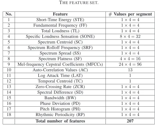
In music genre classification experiments, the extracted fea-tures usually belong into 3 categories, namely timbre, rhythm, and pitch-based ones [1], [2]. In this paper, a combination of descriptors measuring energy, spectral, temporal, perceptual, and pitch characteristics of the music recordings is explored [35]. The complete list of the extracted features can be found in Table II.
The 1st feature measures the energy of the audio signal. Feature 2 is computed by maximum likelihood harmonic matching. Features 3 and 4 refer to the perceptual modeling of the human auditory system [17]. The spectral shape is captured by features 5-9 and 14-15. The temporal properties of the signals are correlated with features 10-13 and 16. Feature 17 describes the amplitude of the maximum peak of the folded histogram [36]. Feature 18 was proposed in [37]. Features 1, 2, 5, 7, 11, and 12 were computed using the definitions of the MPEG-7 audio framework [38]. It should be noted that 24 Mel-frequency cepstral coefficients and 8 specific loudness
TABLE II THE FEATURE SET.
No. Feature #Values per segment
1 Short-Time Energy (STE) 14=4
2 Fundamental Frequency (FF) 14=4
3 Total Loudness (TL) 14=4
4 Specific Loudness Sensation (SONE) 84=32
5 Spectrum Centroid (SC) 14=4
6 Spectrum Rolloff Frequency (SRF) 14=4
7 Spectrum Spread (SS) 14=4
8 Spectrum Flatness (SF) 44=16
9 Mel-frequency Cepstral Coefficients (MFCCs) 244=96
10 Auto-Correlation Values (AC) 13
11 Log Attack Time (LAT) 1
12 Temporal Centroid (TC) 1
13 Zero-Crossing Rate (ZCR) 14=4
14 Spectral Difference (SD) 14=4
15 Bandwidth (BW) 14=4
16 Phase Deviation (PD) 14=4
17 Pitch Histogram (PH) 14=4
18 Rhythmic Periodicity (RP) 14=4 Total number of features 207
sensation (SONE) coefficients are extracted for each audio frame of 10 msec duration.
Except features 10-12, the remaining features are computed on frame basis and their 1st and 2nd moments are exploited by averaging over the frames within each 1 sec long texture window. Similarly, the 1st and 2nd moments of the first-order frame-based feature differences are computed. This explains the factor 4 appearing in Table II. In total, 207 features are extracted from each texture window. All features but the MFCCs are non-negative. Accordingly, they can be employed directly into the NTF. For the MFCCs, their magnitude is retained only. The computation of the aforementioned features every 1 sec yields the tensorVof dimensions100020730.
For comparison purposes, a smaller feature set is also tested, which includes the features extracted by the Music Analysis, Retrieval and Synthesis for Audio Signals (MARSYAS) plat-form [39]. This feature set consists of the 1st order moments of the following timbral features: Spectral Centroid, Spectral Rolloff Frequency, Spectral Difference (also known as spectral flux), and 30 MFCCs per frame, which are averaged over 1 sec texture windows. Thus, the tensor of the MARSYAS features has dimensions10003430.
C. Feature Selection
Careful feature selection is essential for classification. Here, the optimal feature subset maximizes the ratio of the inter-class dispersion over the intra-class dispersion: J = tr(S
1 w
S b
),
wheretr() stands for the trace of a matrix,S
wis the
within-class scatter matrix, andS
bis the between-class scatter matrix.
Details on the computation of S w and
S
b can be found in
any textbook on pattern recognition (e.g. [9]). Because, in our case, the number of distinct subsets having cardinalityI
2
(1I 2
207) is
207! (207 I2)!I2!
, the branch-and-bound search strategy is employed for complexity reduction. In this strategy, a tree structure of(207 I
2
+1)levels is created, where every
node corresponds to a subset. The tree root corresponds to the full set (e.g. 207 features), while each leaf node corresponds to a subset of cardinality I
TABLE IV
AVERAGE ACCURACY ACHIEVED BY SEVERAL CLASSIFIERS WHEN EITHER THE SUBSET OF80SELECTED FEATURES OR THEMARSYASFEATURE
SET WAS EMPLOYED.
Classifier 80 Feature Subset MARSYAS Feature Set
NTF Frobenius 78.9% 68.3%
SVM 77.2% 67.6%
MLP 77.0% 69.1%
NTF KL 70.4% 61.4%
NTF IS 63.6% 55.0%
strategy traverses the structure using a depth-first search with backtracking [9].
In order to apply the feature selection algorithm, the data tensor should be transformed into a matrix by unfolding [6]. Thus, the unfolding V
(2) 2 R
20730 000 +
is computed from tensorV2R
1000207 30 +
. Several feature subsets were derived with respect to maximizingJcomprisingI
2
2f60;70;80;90g
features out of the 207 initial features. The subset comprising 80 features listed in Table III is found to yield the highest music genre classification accuracy, when it is employed in the proposed NTF Frobenius classifier (cf. subsection IV-D). It is seen that 31 out of the 80 selected features are moments of the MFCCs or their first-order differences.
D. Performance Assessment
Experiments were performed by employing various subsets of selected features as well as the MARSYAS feature set using a stratified 10-fold cross validation, which is widely used in genre classification experiments on the GTZAN dataset.
The rank of the 3rd order genre class-dependent tensor V
should satisfy [8] (and references therein)
kmin fI 1
I 2
;I 1
I 3
;I 2
I 3
g: (24)
Since by the experimental protocolI 1 and
I
3 are fixed to 90
and 30, respectively, the inequality (24) implies k 30I 2,
if I 2
90. Various values of k were tested for the NTF
algorithms within the proposed NTF classifier. The highest genre classification accuracy was obtained for the following values of k: k = 55, when the feature subset comprises
I 2
= 60 features; k = 61, when the number of selected
featuresI
2is 70 or 80; and
k=64, whenI 2
=90features are
selected. For the MARSYAS set,kwas set to 22. The number
of termsKtaken into account in (22) was set to 3 for all NTF
classifiers.
The performance of the NTF classifier was compared against that of multilayer perceptron (MLP) and SVMs. In particular, a 3-layered perceptron with the logistic activation function was used. Its training was performed by the back-propagation algorithm with learning rate equal to 0.3 and momentum equal to 0.2 for 500 training epochs. A multi-class SVM multi-classifier with a 2nd order polynomial kernel with unit bias/offset was also tested [40]. The experiments with the aforementioned classifiers were conducted on the matrix unfolding V
(2) 2 R
I 2
30000 +
using 10-fold cross validation, whereI
2
=f60;70;80;90g.
The average music genre classification accuracy achieved by the classifiers over the 10 folds is listed in Table IV, when
Feature Subset Cardinality
C
la
ss
ifi
ca
ti
o
n
A
cc
u
ra
cy
%
SVM MLP NTF Frobenius
60 70 80 90
70 71 72 73 74 75 76 77 78 79 80
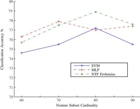
Fig. 3. Average music genre classification accuracy for the various feature subsets.
either the subset of 80 selected features or the MARSYAS feature set was employed. In Figure 3, the average accuracy of the SVM, MLP, and NTF Frobenius classifier is plotted versus several subset cardinalities. From Figure 3, it can be seen that the highest average accuracy of 78.9% was obtained by the proposed NTF Frobenius classifier, when it is applied to the subset of 80 selected features listed in Table III. The standard deviation of the accuracy achieved by the NTF Frobenius classifier is found to be 2.60%. The aforementioned classification accuracy outperforms that reported in [12] (i.e. 61.0%), [3] (i.e. 74.9%), [15] (i.e. 74.0%), and slightly ex-ceeds that reported in [13] (i.e. 78.5%). In [14], a greater classification accuracy than ours is reported (i.e. 82.5%) by employing boosting. However, since cross-validation was not used, the latter accuracy is not directly comparable with ours (i.e. 78.9%). The NTF classifier, when the Frobenius norm was used, attained a higher accuracy than that achieved by the SVM or the MLP for 80 selected features. This was not the case when 60 or 70 features were selected, as can be seen in Figure 3.
Concerning the classification accuracy when the full set of 207 features is used with , it was measured 54.7%, 49.2%, and 40.8% for the NTF Frobenius, NTF KL, and NTF IS classifiers, respectively, with k set to 86. The corresponding
accuracies for the SVM or the MLP classifiers were 51.8% and 53.5%, respectively.
The NTF Frobenius classifier outperforms the SVM for all subset feature cardinalities tested. The NTF classifier achieved a lower accuracy, when either the KL divergence or the IS distance was employed, than that when the Frobenius norm was used.
TABLE III
THE80FEATURES SELECTED BY THE BRANCH-AND-BOUND ALGORITHM.
No. Selected Feature No. Selected Feature
1 Mean of 2nd SF coefficient 41 Mean of 1st order difference of 2nd SF coefficient
2 Variance of 1st SONE 42 Variance of SS
3 Mean of SF 43 Mean of 8th SONE
4 Mean of 2nd SONE 44 Variance of 2nd SF coefficient
5 Mean of BW 45 Variance of 1st order difference of 20th MFCC
6 Variance of 1st order difference of 13rd MFCC 46 Mean of 9th MFCC
7 Mean of 12th MFCC 47 Variance of 1st order difference of 2nd MFCC
8 Mean of SC 48 Mean of 1st order difference of 10th MFCC
9 Mean of 1st SF coefficient 49 Mean of 5th MFCC
10 Mean of SS 50 Mean of 3rd MFCC
11 Variance of TL 51 Variance of 1st order difference of 1st SF coefficient
12 Variance of 1st order difference of 5th MFCC 52 7th AC coefficient
13 Mean of 3rd SF coefficient 53 Mean of SRF
14 Variance of 8th MFCC 54 Variance of 1st order difference of 24th MFCC
15 Variance of SD 55 3rd AC coefficient
16 Mean of RP 56 Variance of 1st order difference of 12th MFCC
17 Variance of PD 57 Mean of 6th SONE
18 Mean of 4th SF coefficient 58 4th AC coefficient
19 Variance of 1st order difference of SS 59 Variance of 9th MFCC
20 Variance of 1st order difference of 8th MFCC 60 Variance of 2nd SONE coefficient
21 Variance of 1st order difference of 11th MFCC 61 Variance of 1st MFCC
22 Variance of 1st order difference of 10th MFCC 62 Mean of 14th MFCC
23 Mean of 11th MFCC 63 Mean of 1st MFCC
24 Variance of 4th SF 64 Variance of 1st order difference of 4th SF coefficient
25 Mean of TL 65 Mean of 2nd MFCC
26 Variance of 1st order difference of 1st SONE 66 Variance of 1st order difference of 3rd SF coefficient 27 Mean of 1st order difference of RP 67 Variance of 1st order difference of 8th SONE coefficient
28 Variance of 3rd SONE 68 Variance of 1st order difference of 5th SONE coefficient
29 Mean of FF 69 Variance of 1st order difference of 3rd SONE coefficient
30 Variance of 1st order difference of 9th MFCC 70 Mean of 1st order difference of 1st SF coefficient
31 Mean of 1st order difference of 11th MFCC 71 Variance of STE
32 Variance of 1st order difference of RP 72 Variance of BW
33 Mean of 13th MFCC 73 Mean of 1st order difference of 12th MFCC
34 Variance of 1st order difference of SC 74 Mean of 16th MFCC
35 Mean of 1st order difference of 14th MFCC 75 Variance of 1st order difference of 7th MFCC
36 Variance of SC 76 Variance of SRF
37 Variance of 2nd MFCC 77 Variance of 1st order difference of 2nd SF coefficient
38 Variance of 1st SF coefficient 78 Variance of 7th MFCC
39 Variance of 3rd SF coefficient 79 Mean of 4th MFCC
40 Variance of 5th SONE 80 Mean of PD
classifier was used with MARSYAS features, the second best accuracy 68.3% was obtained. The superiority of the extracted features over the MARSYAS ones is partially attributed to the fact that the latter features roughly consist a subset of the former ones. For the MARSYAS features, the NTF classifier with either the KL divergence or the IS distance is less performing than the NTF classifier with the Frobenius norm.
Next, the statistical significance of the accuracy differ-ences between the classifiers was addressed by employing the method described in [41], where the number of correctly classified patterns is assumed to be distributed according to the binomial distribution. It can easily be shown that the perfor-mance gains obtained by the NTF Frobenius classifier against the SVM and MLP classifiers are not statistically significant at 95% confidence level. On the contrary, the accuracy difference between the NTF classifier with the Frobenius norm and the
same classifier, when either the KL divergence or the IS distance is used, is found to be statistically significant at 95% confidence level. It should be noted that the difference of 0.4% between the one-vs-the-rest SVMs [13] and the NTF Frobenius classifier is statistically insignificant as well. However, the performance gain obtained by the NTF Frobenius against the classifiers employed in [3], [12], [15] is statistically significant.
TABLE V
AVERAGE CONFUSION MATRIX FOR THENTF FROBENIUS CLASSIFIER USING THE80SELECTED FEATURES OVER THE10SPLITS DETERMINED
BY10-FOLD STRATIFIED CROSS-VALIDATION.
Genre Blues Classical Country Disco Hiphop Jazz Metal Pop Reggae Rock
Blues 86 1 6 1 0 1 0 0 1 4
Classical 1 88 9 0 0 1 0 0 0 1
Country 2 0 87 1 0 3 0 0 1 6
Disco 2 0 4 76 4 0 0 3 3 8
Hiphop 3 0 2 11 67 0 3 5 8 1
Jazz 4 1 10 2 0 77 4 0 0 2
Metal 1 0 0 1 0 1 92 0 0 5
Pop 3 1 3 15 3 0 0 72 1 2
Reggae 2 0 2 5 5 1 0 5 73 7
Rock 4 0 5 4 0 2 7 2 5 71
TABLE VI
AVERAGE CONFUSION MATRIX FOR THESVMCLASSIFIER USING THE80
SELECTED FEATURES OVER THE10SPLITS DETERMINED BY10-FOLD STRATIFIED CROSS-VALIDATION.
Genre Blues Classical Country Disco Hiphop Jazz Metal Pop Reggae Rock
Blues 84 0 4 2 1 2 0 1 2 4
Classical 0 97 1 0 0 1 0 0 0 1
Country 6 2 73 4 0 2 0 1 0 12
Disco 2 0 3 77 2 0 1 4 3 8
Hiphop 2 0 0 8 73 0 2 3 11 1
Jazz 5 5 7 0 1 80 0 0 0 2
Metal 0 0 0 1 3 0 90 1 0 5
Pop 1 1 5 3 3 0 2 77 3 5
Reggae 4 0 1 9 11 1 0 3 67 4
Rock 7 0 17 11 1 0 5 2 3 54
misclassified as either Country or Disco ones. The same occurs for the MLP classifier. It is worth noting that the boundaries between genres such as Pop and Rock as well as Rock and Metal still remain fuzzy [2], a fact that is reflected in the annotations accompanying the dataset.
V. CONCLUSIONS- FUTUREWORK
In this paper, music genre recognition experiments have been performed using a variety of sound description features and multilinear classification techniques. Novel algorithms for the NTF have been derived from first principles and their computational cost has been estimated. An NTF classifier that trains a basis for each class separately and employs basis orthogonalization has also been proposed. The NTF classifier has been tested against state-of-the-art classifiers. It has been found to be slightly superior than them. This superiority is attributed to the higher expressive power of the multilinear representations than that of the pattern matrix the standard pattern recognition algorithms they depend on.
NTF classifiers compared to standard machine learning approaches, such as MLPs and SVMs, are not limited to vec-torized data, but can be used for higher order representations.
TABLE VII
AVERAGE CONFUSION MATRIX FOR THEMLPCLASSIFIER USING THE80
SELECTED FEATURES OVER THE10SPLITS DETERMINED BY10-FOLD STRATIFIED CROSS-VALIDATION.
Genre Blues Classical Country Disco Hiphop Jazz Metal Pop Reggae Rock
Blues 80 3 4 0 0 3 2 1 1 6
Classical 0 93 0 0 0 3 0 1 0 3
Country 3 1 74 3 0 5 0 2 1 11
Disco 4 1 8 72 3 0 2 3 4 3
Hiphop 2 0 1 2 80 0 2 5 7 1
Jazz 9 4 2 0 0 82 1 0 1 1
Metal 1 0 0 2 2 0 87 3 0 5
Pop 1 0 6 3 2 0 1 79 1 7
Reggae 4 0 3 3 9 1 0 3 72 5
Rock 6 0 19 8 1 2 6 2 5 51
For example, tensors can be used for modeling any recording as a time series of potentially different genre labels. NTF offers an attractive framework for modeling data as a multilinear combination of features and can extract basis features enabling a greater interpretability of the basis contributions to the clas-sification than SVMs and MLPs. Such factorizations can also be used for dimensionality reduction prior to the application of standard machine learning algorithms (e.g. SVMs). NTF is not limited to music genre classification, but it can be utilized in various cases associated with feature vectors computed over time, such as for multiple frequency estimation in audio recordings in order to provide a global spectral basis for a whole set instead of a basis for each recording [42].
In the future, the performance of NTF will be assessed on hierarchical music genre databases, which offer additional flexibility over the flat classification approaches. In addition, the NTF algorithms could be enhanced by incorporating penalty functions into the factorization problem, which can control the outcome of the factorization. Finally, various initialization techniques similar to those proposed for the NMF algorithm [44], could be developed for the NTF algorithms aiming to reduce the number of iterations.
APPENDIXI
A. Problem Formulation
As stated in Section III-D, the following minimization problem is treated:
min u
(i) j
0 D
k X
j=1 u
(1) j
Æu (2) j
ÆÆu (n) j
;V
:
Let l = 1;2;:::;I i and
i = 1;2;:::;n. The goal is to find
a multiplicative updating rule for the elements of vectorsu (i) l
denoted asu (i) jl
,j=1;2;:::;k. From (5), it can be seen that:
D
k X
j=1 u
(1) j
Æu (2) j
ÆÆu (n) j
;V
=
I i X
l=1 D
k X
j=1 u
(1) j
Æu (2) j
Æu (i 1) j
u (i) jl
Æu (i+1) j
ÆÆu (n) j
;V %
i =l
(25)
where V %i=l
2 R I
1 I
2 I
i 1 I
i+1 I
N is a sub-tensor
with the ith index fixed to l whose elements are denoted by
v
%1:::%i 1l%i+1:::%n, %
`
=1;2;:::;I `and
`=1;2;:::;i 1;i+ 1;:::;n.
B. Auxiliary function
The minimization problem can be solved using auxiliary functions [11], [23]. Let F(u
(i) l
) denote the divergence term
in (25), i.e.
F(u (i) l
)=D
k X
j=1 u
(1) j
Æu (2) j
Æu (i 1) j
u (i) jl
Æu (i+1) j
ÆÆu (n) j
;V% i
=l
:
The application of (4) and (5) to (26) yields: F(u (i) l )= X % i k X j=1 u (1) j% 1 u (i 1) j% i 1 u (i) jl u (i+1) j% i+1 u (n) j% n (v %1:::%i 1l%i+1:::%n ) (v
%1:::%i 1l%i+1:::%n ) k X j=1 u (1) j%1 u (i 1) j%i 1 u (i) jl u (i+1) j%i+1 u (n) j%n v %1:::%i 1l%i+1:::%n ; (27)
where (x) = 0
(x). The following auxiliary function for F(u
(i) l
)is proposed:
G(u (i) l ; ~ u (i) l )= X %i k X j=1 %1:::j:::%n u (1) j% 1 u (i 1) j% i 1 u (i) jl u (i+1) j% i+1 u (n) j% n % 1 :::% i 1 j% i+1 :::% n ! (v % 1 :::% i 1 l% i+1 :::% n
) (v
% 1 :::% i 1 l% i+1 :::% n ) k X j=1 u (1) j%1 u (i 1) j%i 1 u (i) jl u (i+1) j%i+1 u (n) j%n v %1:::%i 1l%i+1:::%n (28) where % 1 :::% i 1 j% i+1 :::% n = u (1) j% 1 u (i 1) j% i 1 ~ u (i) jl u (i+1) j% i+1 u (n) j% n P k j 0 =1 u (1) j 0 % 1 u (i 1) j 0 % i 1 ~ u (i) j 0 l u (i+1) j 0 % i+1 u (n) j 0 % n : (29)
It can easily be shown that G(u (i) l
;u (i) l
) = F(u (i) l
). In
addition, using Jensen’s inequality for convex functions, it can be verified that G(u
(i) l
;u~ (i) l
)F(u (i) l
). Accordingly, indeed G(u
(i) l
;u~ (i) l
)is an auxiliary function forF(u (i) l
).
C. Minimization of the auxiliary function
In order to derive a multiplicative update rule for u (i) jl
,
the auxiliary functionG(u (i) l
;u~ (i) l
)should be minimized with
respect to u (i) jl
. The partial derivative of G(u (i) l
;u~ (i) l
) with
respect to u (i) jl
is set to zero:
G(u (i) l
;u~ (i) l ) u (i) jl = X % i %1:::%i 1j%i+1:::%n u (1) j%1 u (i 1) j%i 1 u (i) jl u (i+1) j%i+1 u (n) j%n %1:::%i 1j%i+1:::%n u (1) j%1 u (i 1) j%i 1 u (i+1) j%i+1 u (n) j%n %1:::%i 1j%i+1:::%n X %i (v % 1 :::% i 1 l% i+1 :::% n ) u (1) j% 1 u (i 1) j% i 1 u (i+1) j% i+1 u (n) j% n (30)
By replacing (29) into (30) and after performing some alge-braic manipulations, we obtain:
G(u (i) l
;u~ (i) l ) u (i) jl = X %i u (1) j%1 u (i 1) j%i 1 u (i+1) j%i+1 u (n) j%n k X j 0 =1 u (1) j 0 %1 u (i 1) j 0 %i 1 ~ u (i) j 0 l u (i+1) j 0 %i+1 u (n) j 0 %n u (i) jl ~ u (i) jl X % i (v % 1 :::% i 1 l% i+1 :::% n ) u (1) j% 1 u (i 1) j% i 1 u (i+1) j% i+1 u (n) j% n (31) The equation G(u (i) l
;u~ (i) l ) u (i) jl
=0 (32)
cannot be analytically solved for any (). If ()is assumed
to be multiplicative as in [11] (i.e. (xy)= (x) (y)), the
substitution of (31) in (32) yields the following update rule:
u (i) jl ~ u (i) jl 1 P % i (v% 1 :::% i 1 l% i+1 :::% n
)j% 1 :::% i 1 % i+1 :::% n P % i j% 1 :::% i 1 % i+1 :::%n ( % 1 :::% i 1 l% i+1 :::% n ) ! (33) where
j%1:::%i 1%i+1:::%n and
%1:::%i 1l%i+1:::%n are defined in
(12) and (13), respectively. The update rule (33) should be applied to all elementsu
(i) jl
forj =1;2;:::;k,i=1;2;:::;n,
andl=1;2;:::;I
i. It should be noted that
()is
multiplica-tive for the Frobenius norm, since(x)= 1 2 x
2
) (x)=x.
The update rule for the Frobenius norm given in (14) can be easily derived from (33).
However, (33) cannot be applied to the KL divergence or the IS distance, since the associated functions () are not
multiplicative. Indeed, we have (x) =xlog(x) ) (x) =
log(x)+1 for the KL divergence. By replacing the explicit
form of (x) into (31), we obtain
X % i j%1:::%i 1%i+1:::%n log %1:::%i 1l%i+1:::%n +log u (i) jl ~ u (i) jl ! X %i log v % 1 :::% i 1 l% i+1 :::% n j% 1 :::% i 1 % i+1 :::% n =0; (34)
which leads to the update rule (11). Similarly, for the IS distance,(x) = log(x) ) (x) =
1 x
. By replacing the explicit form of (x)into (31), we obtain the update rule (15).
D. Proof of Convergence
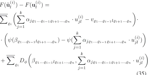
To prove the convergence of the multiplicative update rule for the Frobenius NTF algorithm (14), one needs to show that F(u
(i) l
) F(~u (i) l
). Using the definition of F(u (i) l
),
j%1:::%i 1%i+1:::;%n and
and (13), respectively, it can be shown that:
F(~u (i) l
) F(u (i) l )= X %i k X j=1 j%1:::%i 1%i+1:::;%n u (i) jl v %1:::%i 1l%i+1:::%n ( %1:::%i 1l%i+1:::;%n ) ( k X j=1 j%1:::%i 1%i+1:::;%n u (i) jl ) + X %i D %1:::%i 1l%i+1:::;%n ; k X j=1 j%1:::%i 1%i+1:::;%n u (i) jl : (35)
Since the 2nd term is by definition non-negative, it suffices to prove that the first term in (35) is non-negative. For the Frobenius norm, (x) =x, a fact that facilitates further the
derivations. Moving the denominator in (14) to the left hand side part and summing overj, we get
X %i % 1 :::% i 1 l% i+1 :::;% n v % 1 :::% i 1 l% i+1 :::% n = X %i k X j=1 j% 1 :::% i 1 % i+1 :::;% n u (i) jl % 1 :::% i 1 l% i+1 :::;% n : (36)
Using (36) into the algebraic manipulations of the first term in (35), we conclude that it is sufficient to prove
X %i v % 1 :::% i 1 l% i+1 :::% n k X j=1 j% 1 :::% i 1 % i+1 :::;% n u (i) jl X %i k X j=1 j% 1 :::% i 1 % i+1 :::;% n u (i) jl k X j 0 =1 j 0 % 1 :::% i 1 % i+1 :::;% n u (i) j 0 l (37)
(14) implies that
X %i j%1:::%i 1%i+1:::;%n v %1:::%i 1l%i+1:::%n = X % i j% 1 :::% i 1 % i+1 :::;% n % 1 :::% i 1 l% i+1 :::;% n u (i) jl ~ u (i) jl (38)
Using (38), the inequality (37) is rewritten as
X % i k X j=1 j% 1 :::% i 1 % i+1 :::;% n [u (i) jl ℄ 2 ~ u (i) jl ! % 1 :::% i 1 l% i+1 :::;% n X % i k X j=1 j%1:::%i 1%i+1:::;%n u (i) jl k X j 0 =1 j 0 %1:::%i 1%i+1:::;%n u (i) j 0 l (39)
Inequality (39) holds thanks to Lemma 4 [11], which con-cludes the proof.
APPENDIXII
The computational cost of the NTF is derived forn=3(3rd
order tensors), when the Frobenius norm is used. We assume that one flop corresponds to a single floating point operation, i.e. a floating point addition or a floating point multiplication [43]. The computational cost is detailed in Table VIII. We explicitly calculate the cost for the computation of the matrix
U (1) 2R I 1 k
having columns u (i) j
. The first entry refers to terms
j%2%3defined by (12), which are kI
2 I
3in total and each
of them requires 1 multiplication. The second entry refers to terms
l% 2
% 3
defined by (13), which are I 1
I 2
I
3 in total and
each of them requires2k multiplications andk 1additions.
The cost for one update ofu (1) jl
given by (14) is2(I 2
I 3
+1)
multiplications and 2(I 2
I 3
1) additions, therefore in total 4I
2 I
3. There are I
1
k elements that should be computed. In
total, one needs(7k 1)I 1 I 2 I 3 +kI 2 I
3 flops per iteration in
order to compute the full matrixU (1)
. By repeating the same computation forU
(2)
andU (3)
and multiplying by the number of iterationsr needed for convergence, we obtain:
3r(7k 1)I 1 I 2 I 3 +rk(I 2 I 3 +I 1 I 3 +I 1 I 2 ): (40)
It can be said that the Itakura-Saito NTF and the Kullback-Leibler NTF algorithms have a computational cost of the same order to that given by (40), if a constant cost is assumed for the computation of logarithms and exponentials.
The inspection of (40) reveals that the cost of the non-negative training tensorV
factorization depends linearly on
the number of the training recordingsI
1for each genre class.
Besides the NTF, the computational cost of the proposed NTF classifier training in Section III-E involves tensor unfolding (of no cost), the Khatri-Rao matrix productU
(3)
U (2) , its QR
decomposition, and the matrix productH =R [U (1) ℄ T for each genre. The just mentioned Khatri-Rao matrix product is computed at a cost ofI
3 I
2
kflops. The QR decomposition can
be performed at a cost of2I 3
I 2
k 2
flops, if the modified Gram-Schmidt method is used [43].H
can be computed at a cost
ofI 1
(2k 1)kflops. The test phase involves (20)-(22), which
implies a computational cost ofO(I 1
k 2
[image:12.595.50.303.123.252.2] [image:12.595.50.556.410.757.2])for each genre.
TABLE VIII
3RD ORDERFROBENIUSNTF COMPUTATIONALCOST.
Term Flops j%2%3 I 2 I 3 k l%2%3 (3k 1)I 1 I 2 I 3 u (1) jl
givenj%2%3andl%2%3 4I1I2I3k
U (1)
per iteration (7k 1)I1I2I3+kI2I3
U (i)
,i=1;2;3, per iteration 3(7k 1)I1I2I3+k(I2I3+I1I3+I1I2)
Frobenius NTF forriterations 3r(7k 1)I1I2I3+rk(I2I3+I1I3+I1I2)
REFERENCES
[1] J.-J. Aucouturier and F. Pachet, “Representing musical genre: a state of the art,” J. New Music Research, Vol. 32, No. 1, pp. 83-93, 2003. [2] N. Scaringella, G. Zoia, and D. Mlynek, “Automatic genre classification
of music content,” IEEE Signal Processing Mag., Vol. 23, No. 2, pp. 133-141, March 2006.
[3] T. Lidy and A. Rauber, “Evaluation of feature extractors and psycho-acoustic transformations for music genre classification,” in Proc. 6th Int.
[4] D. Perrott and R. O. Gjerdingen, “Scanning the dial: An exploration of factors in the identification of musical style,” Dept. Music, Northwestern
University, Illinois, Res. Notes, 1999.
[5] C. McKay and I. Gujinaga, “Musical genre classification: is it worth pursuing and how can it be improved?,” in Proc. 7th Int. Conf. Music
Information Retrieval, pp. 34-41, September 2006.
[6] L. De Lathauwer, “Signal Processing Based on Multilinear Algebra”, Ph.D. thesis, K.U. Leuven, E.E. Dept.-ESAT, Belgium, 1997. [7] D. C. Kay, Theory and Problems of Tensor Calculus, New York:
McGraw-Hill, 1988.
[8] T. G. Kolda and B. W. Bader: “Tensor Decompositions and Applica-tions,” SIAM Review, Vol. 51, No. 3, to appear.
[9] F. van der Heijden, R. P. W. Duin, D. de Ridder, and D. M. J. Tax,
Classification, Parameter Estimation and State Estimation, London UK:
Wiley, 2004.
[10] L. M. Bregman, “The relaxation method of finding the common points of convex sets and its application to the solution of problems in convex programming,” USSR Computational Mathematics and Mathematical
Physics, Vol. 7, pp. 200-217, 1967.
[11] S. Sra and I. S. Dhillon, “Nonnegative matrix approximation: algorithms and applications,” Technical Report TR-06-27, Computer Sciences, Uni-versity of Texas at Austin, 2006.
[12] G. Tzanetakis and P. Cook, “Musical genre classification of audio signals,” IEEE Trans. Speech and Audio Processing, Vol. 10, No. 5, pp. 293-302, July 2002.
[13] T. Li, M. Ogihara, and Q. Li, “A comparative study on content-based music genre classification,” in Proc. 26th Annual ACM Conf. Research
and Development in Information Retrieval, pp. 282-289, July-August
2003.
[14] J. Bergstra, N. Casagrande, D. Erhan, D. Eck, and B. Kegl: “Aggregate Features and AdaBoost for Music Classification,” Machine Learning, Vol. 65, No. 2-3, pp. 473–484, 2006.
[15] A. Holzapfel and Y. Stylianou, “Musical genre classification using nonnegative matrix factorization-based features,” IEEE Trans. Audio,
Speech, and Language Processing, Vol. 16, No. 2, pp. 424-434, February
2008.
[16] P. Cano, E. G ´omez, F. Gouyon, P. Herrera, M. Koppenberger, B. Ong, X. Serra, S. Streich, and N. Wack, “ISMIR 2004 audio description contest,”
MTG Technical Report: MTG-TR-2006-02, 2006.
[17] E. Pampalk, A. Flexer, and G. Widmer, “Improvements of audio based music similarity and genre classification,” in Proc. 6th Int. Symp. Music
Information Retrieval, pp. 628-633, 2005.
[18] J. J. Burred and A. Lerch, “A hierarchical approach to automatic musical genre classification,” in Proc. 6th Int. Conf. Digital Audio Effects
(DAFx), September 2003.
[19] A. Meng, P. Ahrendt, and J. Larsen, “Improving music genre classifi-cation by short-time feature integration,” in Proc. 6th Int. Symp. Music
Information Retrieval, pp. 604-609, September 2005.
[20] J. G. A. Barbedo and A. Lopes, “Automatic genre classification of musical signals,” EURASIP Journal on Advances in Signal Processing, Vol. 2007, Article ID 64960, 2007.
[21] Z. Cataltepe, Y. Yaslan, and A. Sonmez, “Music genre classification using MIDI and audio features,” EURASIP Journal on Advances in
Signal Processing, Vol. 2007, Article ID 36409, 2007.
[22] P. Paatero, U. Tapper, R. Aalto, and M. Kulmala. “Matrix factoriza-tion methods for analysing diffusion battery data,” Journal of Aerosol
Science, Vol. 22 (Supplement 1), pp. 273-276, 1991.
[23] D. D. Lee and H. S. Seung, “Algoritnms for non-negative matrix factorization,” Advances in Neural Information Processing Systems, Vol. 13, pp. 556-562, 2001.
[24] S. Z. Li, X. Hou, H. Zhang, and Q. Cheng, “Learning spatially localized, parts-based representation,” in Proc. IEEE Conf. Computer Vision and
Pattern Recognition, pp. 1-6, 2001.
[25] N. D. Sidiropoulos, “ Low-rank decomposition of multi-way arrays: A signal processing perspective,” in Proc. Sensor Array and Multichannel
Signal Processing Workshop, pp. 52-58, July 2004.
[26] A. Shashua and T. Hazan, “Non-negative tensor factorization with applications to statistics and computer vision,” in Proc. 22nd Int. Conf.
Machine Learning, pp. 792-799, August 2005.
[27] T. Hazan, S. Polak, and A. Shashua, “Sparse image coding using a 3D non-negative tensor factorization,” in Proc. 10th IEEE Int. Conf.
Computer Vision, Vol. 1, pp. 50-57, October 2005.
[28] C. Boutsidis, E. Gallopoulos, P. Zhang, and R. Plemmons, ”PALSIR: A new approach to nonnegative tensor factorization”, Poster presented at
Workshop Algorithms for Modern Massive Data Sets, June 2006.
[29] M. Heiler and C. Schn¨orr, “Controlling sparseness in non-negative tensor factorization,” in Proc. 9th European Conf. Computer Vision, Vol. 1, pp. 56-67, May 2006.
[30] A. Cichocki, R. Zdunek, S. Choi, R. Plemmons, and S. Amari, “Non-negative tensor factorization using alpha and beta divergences,” in Proc.
2007 IEEE Int. Conf. Acoustics, Speech, and Signal Processing, Vol. III,
pp. 1393-1396, April 2007.
[31] A. Cichocki, R. Zdunek, S. Choi, R. Plemmons, and S. Amari, “Novel multi-layer nonnegative tensor factorization with sparsity constraints,” in Proc. 8th Int. Conf. Adaptive and Natural Computing Algorithms, pp. 271-280, April 2007.
[32] S. Zafeiriou, “Discriminant non-negative matrix factorization algo-rithms,” IEEE Trans. Neural Networks, Vol. 20, No. 2, pp. 217-235, February 2009.
[33] E. Benetos and C. Kotropoulos, “A tensor-based approach for automatic music genre classification,” in Proc. 16th European Signal Processing
Conf., August 2008.
[34] E. Benetos, M. Kotti, and C. Kotropoulos, “Large scale musical in-strument identification,” in Proc. 4th Sound and Music Computing
Conference, pp. 283-286, July 2007.
[35] G. Peeters, “A large set of audio features for sound description (similarity and classification) in the CUIDADO project,” CUIDADO IST Project
Report, 2004.
[36] G. Tzanetakis, A. Ermolinskyi, and P. Cook, “Pitch Histograms in Audio and Symbolic Music Information Retrieval,” J. New Music Research, Vol. 32, No. 2, pp. 143-152, 2003.
[37] E. Pampalk, S. Dixon, and G. Widmer, “Exploring Music Collections by Browsing Different Views,” Computer Music J., Vol. 28, No. 2, pp. 49-62, June 2004.
[38] MPEG-7, “Information Technology-Multimedia Content Description Interface-Part 4: Audio,” ISO/IEC JTC1/SC29/WG11 N5525, March 2003.
[39] G. Tzanetakis, Music Analysis, Retrieval and Synthesis for Audio
Sig-nals, http://marsyas.sness.net/.
[40] B. Sch¨olkopf, C. J. C. Burges, and A. J. Smola, Advances in Kernel
Methods: Support Vector Learning, Cambridge MA, USA: MIT Press,
1999.
[41] I. Guyon, J. Makhoul, R. Schwartz, and V. Vapnik, “What size test set gives good error rate estimates?,” IEEE Trans. Pattern Analysis and
Machine Intelligence, vol. 20, no. 1, pp. 52-64, January 1998.
[42] P. Smaragdis and J. Brown, “Non-negative matrix factorization for polyphonic music transcription,” in Proc. IEEE Workshop Applications
of Signal Processing to Audio and Acoustics, pp. 177-180, 2003.
[43] G. H. Golub and C. F. Van Loan, Matrix Computations, 3rd ed., Baltimore, MD: Johns Hopkins Univ. Press, 1996.