Reuleaux plasticity: Analytical backward Euler stress integration and consistent tangent

City, University of London Institutional Repository

Citation

: Coombs, W.M., Crouch, R.S. and Augarde, C.E. (2010). Reuleaux plasticity:

Analytical backward Euler stress integration and consistent tangent. Computer Methods in

Applied Mechanics and Engineering, 199(25-28), pp. 1733-1743. doi:

10.1016/j.cma.2010.01.017

This is the accepted version of the paper.

This version of the publication may differ from the final published

version.

Permanent repository link:

http://openaccess.city.ac.uk/15548/

Link to published version

: http://dx.doi.org/10.1016/j.cma.2010.01.017

Copyright and reuse:

City Research Online aims to make research

outputs of City, University of London available to a wider audience.

Copyright and Moral Rights remain with the author(s) and/or copyright

holders. URLs from City Research Online may be freely distributed and

linked to.

City Research Online: http://openaccess.city.ac.uk/ [email protected]

Reuleaux plasticity: Analytical backward Euler stress integration and

consistent tangent

William M. Coombs, Roger S. Crouch

⁎

, Charles E. Augarde

School of Engineering and Computing Sciences, Durham University, South Road, Durham, DH1 3LE, United Kingdom

a b s t r a c t

Analyticalbackward Eulerstressintegration ispresentedfora deviatoricyieldingcriterion basedona modifiedReuleauxtriangle.Thecriterionisappliedtoaconemodelwhichallowscontrolovertheshapeof thedeviatoricsection,independentoftheinternalfrictionangleonthecompressionmeridian.Thereturn strategyandconsistenttangentarefullydefinedforallthreeregionsofprincipalstressspaceinwhichelastic trialstatesmaylie.Errorsassociatedwiththeintegrationschemearereported.Theseareshowntobeless than3%forthecaseexamined.Runtimeanalysisrevealsa2.5–5.0timesspeed-up(atamaterialpoint)over the iterative Newton–Raphson backward Euler stress return scheme. Two finite-element analyses are presenteddemonstrating thespeedbenefitsofadoptingthisnew formulationinlargerboundaryvalue problems.ThesimplemodifiedReuleauxsurfaceprovidesanadvanceoverMohr–CoulombandDrucker–

Prager yieldenvelopes in thatit incorporatesdependencies onboththe Lode angleand intermediate principalstress,withoutincurringtheruntimepenaltiesofmoresophisticatedmodels.

1. Introduction

While a vast body of constitutive models has been generated over the last decades, very few of the advanced formulations have gained widespread use. This has been largely a consequence of their computational burden. Developing algorithmically efficient and fully robust constitutive models for engineering materials has therefore become just as important as providing realism, in order to allow detailed three dimensional non-linear deformation analyses to be undertaken.

In this paper we offer a simple cone-type (frictional) elasto-plastic formulation, which allows an analytical backward Euler (BE) stress integration on the curved surface and exact integration in the regions where singularities appear. The BE scheme gives a fully implicit approximation. The popularity of this approach over explicit schemes (for example[15]) is due to its high level of accuracy for a given numerical effort, particularly when large strain increments are applied

[13]. The associated perfect plasticity model presented here may be thought of as a simple hybrid sitting between the Drucker–Prager (D–P) and Mohr–Coulomb (M–C) formulations. The D–P yield surface exhibits no Lode angle dependency,θ. The M–C surface has no sensitivity to the intermediate principal stress,σ2. Yet multiaxial experiments show that

both factors influence yielding and peak stress. Their inclusion in constitutive models appears necessary in order to capture the deformation of geotechnical structures [2]. The attraction of the

proposed model is the improved fit to deviatoric yielding (the formulation has a sensitivity toθandσ2) and a one-step integration

scheme. The consequences of neglecting Lode angle andσ2

dependen-cies are discussed further inSection 2.

The layout of the paper is as follows. InSection 2the particular form of the deviatoric section is introduced.Section 3describes the stress return strategies for the three regions where the elastic trial stress may lie. The approach, when returning to the compression meridian or tensile apex, follows Clausen et al.'s method[4]. When returning elsewhere,finding the closest point to the surface in energy-mapped space[5]requires the solution of a quartic.Section 3also gives the consistent tangent ex-pressions for each region and quanti_fies the errors associated with the analytical stress return.Section 4presents a run time comparison be-tween the standard iterative BE stress return and the proposed analytical single-step return. Two finite-element simulations are presented in

Section 5. The analysis of a single 3D finite-element toy problem illustrates the asymptotic quadratic convergence of the global Newton– Raphson (N–R) solution scheme. A larger, rigid footing plane-strain

finite-element, analysis compares solutions obtained from the proposed model with those obtained from D–P, M–C and Willam–Warnke (W–W

[16]) cones. A number of other forms of Lode angle dependencies on the yield surface have been proposed in the literature[1,3,10,17]. These can improve on the relatively poorfit of the D–P and M–C idealisations, yet none offer the advantage of a closed form BE integration solution which is available for the formulation proposed here.

vector transpose. We adopt a tension positive convention and assume the following ordering of the principal stressesσ1 ≤ σ2 ≤ σ3.

2. Modified Reuleaux

For the plasticity models under consideration, the yield surfaces may be defined using Haigh–Westergaard cylindrical coordinatesξ,ρ

andθ. The normalised deviatoric radius,ρ ̅=ρ/ρc, is employed; where

ρcis the radius on the compression meridian (θ=π/6) and ρis a function of the Lode angleθ∈[−π/6,π/6]

θ= 1

3arcsin

−3pffiffiffi3 2

J3

J3₂=2 !

: ð1Þ

HereJ2=(tr[s]2)/2,J3=(tr[s]3)/3,½s=½σ−ξ½1=

ffiffiffi

3

p

,ξ= tr½σ=pffiffiffi3 and [1] denotes the third-order identity matrix.

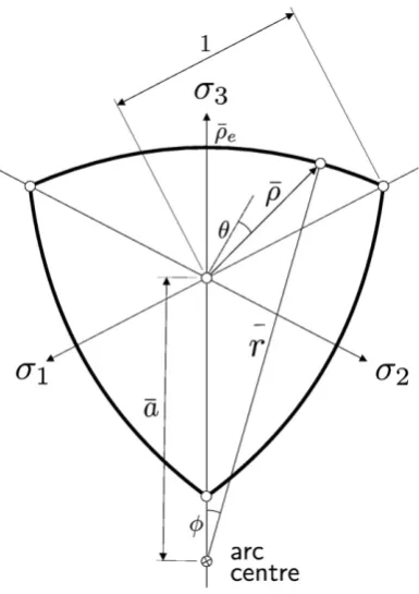
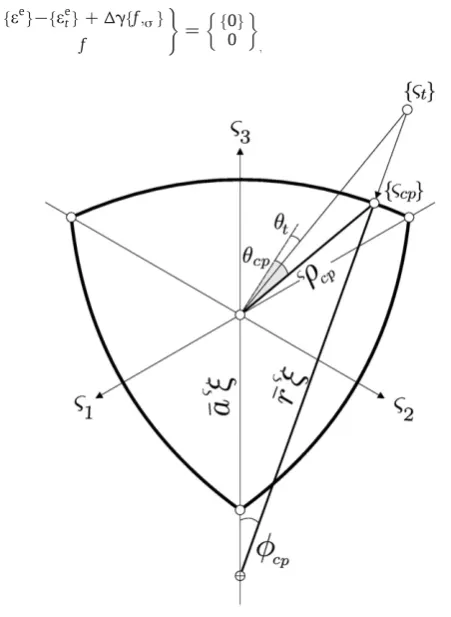
From geometric considerations (seeFig. 1) the modi_fied Reuleaux (MR) Lode angle dependency may be obtained as

ρðθÞ=

ffiffiffiffiffiffiffiffiffiffiffiffiffiffiffiffiffiffiffiffiffiffiffiffiffiffiffiffiffiffiffiffiffiffiffiffiffiffiffiffiffiffiffiffiffi a2_+r2

−2a rcosðϕÞ

q

; ð2Þ

where

¯

r= ¯ρ 2

e−¯ρe+ 1

2ρ¯e−1 ;

a=r_−¯ρeand ρ¯e=ρe ρc:

ð3Þ

ρ ̅e∈[0.5,1] gives the relative size of the radius under triaxial extension (σ1=σ2bσ3) with respect to that under triaxial compression

(σ1bσ2=σ3). The arc angle,ϕ, is defined as

ϕ= π

6 +θ−arcsin ¯

asinð5_π=6_−θÞ

¯

r

:

ð4Þ

If the arc centres coincide with the singularities on the compression meridians (that is, if r_̅= 1+ _¯ρeso that a̅= 1) then

the shape of the deviatoric section is a Reuleaux triangle. Although this shape was used in cam-actuated steam engine regulators in the 1830s, the_first written discussion of the geometry appears to have been provided by Franz Reuleaux in 1876, when considering a family of curved shapes of constant breadth (that is, rolling poly-gons which maintain a constant height)[9,11]. Allowing the loca-tion of the arc centres to vary along projecloca-tions of the compression meridians gives rise to themodified Reuleaux triangle. Asρ ̅e→0.5 both r̅ and a̅ tend to ∞ and the deviatoric section becomes an equilateral triangle. If ρ ̅e= 1 thenρ ̅= 1 and we recover a circular deviatoric section centred on the hydrostatic axis (as found in the D–P model).

Fig. 2 compares the proposed deviatoric section with those attributed to M–C, W–W and Bhowmik–Long (B–L, [3], with a normalised deviatoric radius of ρ ̅s= 0.73 on the shear meridian,

θ= 0) for_{ρ ̅}e= 0.656. The multiaxial experimental data on Monterey sand[8]shown in thefigure indicate that this material has both a Lode angle dependency (Fig. 2(A)) and a sensitivity to the intermediate principal stress (Fig. 2(B)). Unlike the other models mentioned above, a D–P surface provides no variation in ρ ̅with respect toθ(ρ ̅would Fig. 1.Modified Reuleaux triangle definition.

equal 1 in Fig. 2(A)). The effective friction angle in Fig. 2(B) is calculated from the expression given by Griffiths

ψ= arcsin

ffiffiffi

3

p

ηcosðθÞ

ffiffiffi

2

p

+ηsinðθÞ

!

; ð5Þ

where η=ρ/ξ [7]. In that Figure, the M–C envelope exhibits no sensitivity toσ2. It is evident that the proposed MR deviatoric section

offers an improved fit over the D–P and M–C surfaces while maintaining a relatively simple mathematical form. Although the W–W and B–L envelopes provide more satisfactory fits to the experimental data when the intermediate stress ratio 0.5bbb0.95 (where b= (σ2−σ3)/(σ1−σ3)), neither the W–W nor the B–L

model are able to offer analytical BE stress integration solutions for arbitrary strain increments. Thus they can incur significant compu-tational overheads (compared with D_–P and M_–C models) when introduced into a large-scale elasto-plastic stress analysis. It is worth adding that a number of geotechnical problems satisfy plane-strain conditions, wherebtypically lies close to 0.3[12]. The MR solution provides a goodfit to the multiaxial data in this region.

The MR cone can be defined as

fðη;θÞ=α¯ρ−η= 0 ð6Þ

whereαis the opening angle of the cone,α=−tan(ψMC).ψMCis the

M–C internal friction angle of the material under triaxial compression. Thus Eq. (6) defines a cone with a MR deviatoric section and linear meridians, pinned at the stress origin with the space diagonal (σ1=σ2=σ3) as the cone's axis, see Fig. 3. The MR cone can be

seen as a hybrid surface, lying between the D_–P and M_–C envelopes, allowing some control over the shape of the deviatoric section, independent of the cone opening angle.

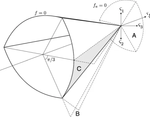
3. Stress return and consistent tangent

Consider the trial elastic stress {σt} (given by a trial elastic strain {εte}) lying outside the yield surface (f N0). For this state there are three distinct stress return regions associated with the MR cone, as shown inFig. 3, namely:

A. Return to the stress origin (point), B. return to the compression meridian (line), C. return to the non-planar surface.

The Closest Point Projection (CPP) and consistent tangent are considered for each region inSections 2–4.Table 1gives the pseudo-code for the stress return algorithm.

3.1. Energy-mapped stress space

Simo and Hughes[13]showed that the BE integration corresponds to the minimisation of

fσrg−fσtg

f gT

½Ce ff σrg−fσtgg; ð7Þ

with respect to the return stress {σr} (where [Ce] is the elastic compliance matrix), which represents a CPP. The minimisation is subject to the following constraints

f ≤0; γ˙ ≥0; fγ˙ = 0: ð8Þ

(_⋅)tand (⋅)rdenote quantities associated with the trial state and the return state respectively, wherefis the yield function andγ̇is the plastic multiplier. The return stress is not generally the closest point geometrically in standard stress space, but rather the stress that minimises the energy square norm Eq. (7). In this paper we make use of energy-mapped {ς} space[5], where

1

Efςg

T ς

f g=fσgT

½Cef gσ ; ð9Þ

andEis the Young's modulus of the elastically isotropic material. This allows us tofind the geometric closest point (in {ς} space) through use of the following transformation

fςg=½Tfσg: ð10Þ

For isotropic linear elasticity, [T] is solely a function of Poisson's ratio_υ. Given the elastic compliance matrix

Ce =1

E

1 −v −υ 0 0 0

−υ 1 −υ 0 0 0

−υ −υ 1 0 0 0 0 0 0 2ð1 +υÞ 0 0 0 0 0 0 2ð1 +υÞ 0 0 0 0 0 0 2ð1 +υÞ

2 6 6 6 6 6 6 4 3 7 7 7 7 7 7 5 ;

ð11Þ

[T] becomes

T

½ =

t1 t2 t2 0 0 0

t2 t1 t2 0 0 0

t2 t2 t1 0 0 0 0 0 0 t3 0 0 0 0 0 0 t3 0 0 0 0 0 0 t3

2 6 6 6 6 6 6 4 3 7 7 7 7 7 7 5 ;

ð12Þ

where

t1=

ffiffiffiffiffiffiffiffiffiffiffiffiffi

1−2υ

p

+ 2pffiffiffiffiffiffiffiffiffiffiffiffiffiffi1 +υ

3 ; t2=

ffiffiffiffiffiffiffiffiffiffiffiffiffi

1−2υ

p

−pffiffiffiffiffiffiffiffiffiffiffiffiffiffi1 +υ

3 ; t3=

ffiffiffiffiffiffiffiffiffiffiffiffiffiffiffiffiffiffiffiffiffi

2ð1 +υÞ:

p

ð13Þ

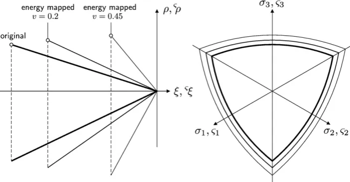
This mapping leads to a squashing and a stretching of the yield surface in the hydrostatic and deviatoric directions respectively (seeFig. 4).

ς

ξ=ξpffiffiffiffiffiffiffiffiffiffiffiffiffi1−2υ; ςρ=ρpffiffiffiffiffiffiffiffiffiffiffiffiffiffi1 +υ; ςθ=θ; ð14Þ

whereς(⋅) denotes a quantity associated with energy-mapped space. The energy-mapped opening angle of the cone,ςα, is

ς_α= α ffiffiffiffiffiffiffiffiffiffiffiffiffiffi1 +υ

p

ffiffiffiffiffiffiffiffiffiffiffiffiffi

1−2υ

p

::

ð15Þ

Once the closest point solution in energy-mapped stress space has been found, the solution can be transformed back to conventional stress space. Note that we need only operate with principal stresses (conventional and energy-mapped) in the solution process for an isotropic model.

3.2. Stress origin return

Iffab0 then the trial stress point {ςt} will be returned onto the apex of the MR cone, with

fςcpg=fσcpg=f0g; ð16Þ

where (⋅)cpdenotes quantities associated with the closest point. The apex yield function is given by

fa=ςρ_αþςη= 0: ð17Þ

3.2.1. Stress origin consistent tangent

As Clausen et al. [4] have shown, the elasto-plastic consistent tangent for a hydrostatic apex return is simply given by

½Dalg=½0: ð18Þ

3.3. Compression meridian return

The trial arc angleϕtshould be checked againstϕcrto determine if the trial point returns onto the compression meridian, where

ϕcr= arcsin

ffiffiffi

3

p

2r !

:

: ð19Þ

If_ϕt≥ϕcrthen

θcp=π=6; ςρcp=ςαςξcp:

One obtains the solution for this case by considering a plane normal to the compression meridian of the energy-mapped yield surface. The closest point and trial point will lie in the same normal plane. We make use of

fςngT

ffςcpg−fςtgg= 0 ð20Þ

where {ςn} is the normal to the plane; which in this case is the vector defining the corner line of the energy-mapped yield surface. {ςn} is given by

fςng= 1n −pffiffiffi2ςα 1þςα=p2ffiffiffi 1þςα=pffiffiffi2oT

; ð21Þ

and any {ς} on this line is given by

ς

f g= ς_ξ

ffiffiffi

3

p n1−pffiffiffi2ςα 1þς_α=pffiffiffi_{2 1þ}ς_α=pffiffiffi₂oT

:: ð22Þ

Substituting Eqs. (21) and (22) into Eq. (20) we obtain an equation which can be solved forςξcp

ς

ξcp=

ςt2 +ςt3

1þς_α=pffiffiffi₂

+ςt1 1−

ffiffiffi

2

p _ς

α

ffiffiffi

3

p

1þς_α2

:

ð23Þ

Subsequentlyςξcpandςρcpcan be transformed back into conven-tional stress space to calculate thefinal return stress {σcp} using the Haigh–Westergaard solution

σ

f g= ξffiffiffi 3

p f g1 +

ffiffiffi

2 3

r

ρfsinðθ−2π=3ÞsinðθÞsinðθ+ 2π=3ÞgT ; ð24Þ where {1} = {1 1 1}T_{. These stresses are then transformed back from} principal to generalised stress space through use of the eigenvectors associated with the generalised trial stress state.

3.3.1. Compression meridian consistent tangent

The consistent tangent for a corner return is obtained following the approach given by Clausen et al. [4]. By considering the vector orientation of the edge

fng= 1n −pffiffiffi2α 1 +α=pffiffiffi2 1 +α=pffiffiffi2oT

; ð25Þ

we obtain the third-order elasto-plastic tangent matrix (in principal form) as

ˆ

Dep h i

= fngfng

T

fngT_½Cˆe_f

ng_; ð26Þ

where [Ĉe_{] is the third-order (principal) elastic compliance matrix.}

The generalised (sixth-order) elasto-plastic tangent matrix is then given by

Dep

= ½Dˆep ½0

½0 ðE=2ð1 +υÞÞ½1

:

ð27Þ

The consistent tangent follows as

½Dalg=½Q½Dep; ð28Þ

where [Q] is calculated from

½Q= ½I+Δγ½Ce−1 ∂2f

∂σ2

cp

" #!₋1

;

ð29Þ

where [I] is the sixth-order identity matrix [4]. In principal stress space [Q] can be calculated as

½Q= ½1 ½0

½0 ½―Q

;

ð30Þ

where

½―Q=

1 + Δσ

p

1−Δσ

p

2

σ1−σ2

0 0

0 1 + Δσ

p

2−Δσ

p

3

σ2−σ3

0

0 0 1 + Δσ

p

1−Δσ

p

3

σ1−σ3

2 6 6 6 6 6 6 6 6 6 4

3 7 7 7 7 7 7 7 7 7 5

−1

:

ð31Þ

{Δσp_{} =Δγ[C}e_]−1_{f,

σ} = {σt}−{σcp} is the plastic stress corrector increment associated with the return path. Using the fact thatσ2=σ3

for a return onto the corner, [Q̅] can be simplified to

½―Q=

σ1−σ2

σt1−σt2

0 0

0 0 0

0 0 σ1−σ3

σt1−σt3

2 6 6 6 6 6 4

3 7 7 7 7 7 5

;

ð32Þ

whereσtiare the principal trial stresses. From Eqs. (28) and (32) the

consistent tangent, for the line return, can be written as

½Dalg= ½Dˆep ½0

½0 ðE=2ð1 +υÞÞ½―Q

: ð33Þ

Once the consistent tangent has been formed in principal stress space (Eq. (33)) it must be transformed back to generalised stress space, see Clausen et al. for more details[4].

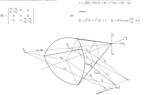
3.4. Non-planar surface return

If we consider an elastic trial stress {ςt}, outside the yield surface, returning onto the non-singular portion of the surface, we can define a lengthlas the distance between that trial point and a point on the surface at the sameφtin any deviatoric plane at a givenςξ (seeFig. 5)

l2=ðrt−rÞ

2

+ðςξ−ςξtÞ

2

; ð34Þ

wherer= r̅ς_ας_{ξ. The deviatoric distance of the trial point from the} arc axis is given by

rt2=a

2

þςρ2

t−2aςρtcos

5π

6−θt

; ð35Þ

wherea= a_̅ς_ας_ξ. Substituting Eqs. (35) and (3) into Eq. (34), we obtain

l= ffiffiffiffiffiffiffiffiffiffiffiffiffiffiffiffiffiffiffiffiffiffiffiffiffiffiffiffiffiffiffiffiffiffiffiffiffiffiffiffiffiffiffiffiffiffiffiffiffiffiffiffiffiffiffiffiffiffiffiffiffiffiffiffiffiffiffiffiffiffiffiffiffiffiffiffiffiffiffiffiffiffiffiffiffiffiffiffiffiffiffiffiffiBς_1ξ2₋₂ς_ξς_ξ

t+B2+rςαrt

ð Þ þς_ξ2

tþςρ2t

q

; ð36Þ

where

B1=a 2ς

α2

+r2ςα2

+ 1; B2=aςαςρtcos

5π

6 −θt

: ð37Þ

Equating the partial derivative of Eq. (36) with respect toςξto zero, we obtain the closest point on the MR cone to the trial point in {ς} space

ς_ξ4

cpA1þςξ 3

cpA2þςξ 2

cpA3þςξcpA4+A5= 0; ð38Þ where

A1=a 2ς

α2_B2 1−4a

4_r2ς α6

; A2= 12a

2

r2ςα4

B2−2a 2ς

α2

B1ðςξt+B2Þ−2B 2 1B2;

A3=a 2ς

α2_ðς_ξ t+B2Þ

2

+B21ρ 2

t+ 4B1B2ðςξt+B2Þ−9r 2ς

α2

B22−4a 2

r2ςα4ς_ρ2

t;

A4= 6r2

ς α2ς_ρ2

tB2−2B1ðςξt+B2Þςρ2t−2B2ðςξt+B2Þ2;

A5=ςρ 2

tðςξt+B2Þ 2

−ς_ρ4

tr

2ς α2

:

ð39Þ

This quartic can be solved forςξcp, see Simo and Hughes page 138

[13], amongst others, for more details. Onceςξcpis known, then the other quantities identifying the position of the closest point on the MR surface can be calculated (Fig. 6).ϕcpis given by the sine rule

ϕcp= arcsin

ς_ρ

tsinð5π=6−θtÞ

rt

!

;

ð40Þ

wherertis calculated at the solutionςξcpusing Eq. (35).ςρcpis given by Eq. (2) andθcpis determined from the cosine rule

θcp=

5π

6 −arccos

a2cpþςρ

2

cp−r

2

cp

2aςcpρcp

!

;

ð41Þ

wherercpandacpare values associated withςξcp.

3.4.1. Non-planar consistent tangent

The consistent tangent for the surface return is calculated by minimising

fεe

g−fεe

tg+Δγff;σg f

( )

= f0g 0

;

ð42Þ

with respect to {εte}, thereby obtaining

½Ce+Δγ½f;σσ ff;σg

ff;σgT 0

fdσg

dΔγ

= fdε e

tg

0

( )

:

ð43Þ

Rearranging we have

fdσg

dΔγ

= ½D

alg _f

D12g

fD21g D22

_fdεe

tg

0

( )

;

ð44Þ

where (⋅),σand (⋅),σσ, in Eqs. (42) and (43), denote the first and second partial derivatives of (⋅) with respect to {σ}. Recalling Eq. (6), thefirst derivative offwith respect to {σ} is given by

ff;σg=αfρ;σg−fη;σg; ð45Þ where

η;σ

f g= fρ;σgξ−ρfξ;σg

ξ2 : ð46Þ

Operating only with the derivatives with respect to the principal stresses, we obtain

fρ;σg=fsg=ρ; fξ;σg=f1g=

ffiffiffi

3

p

: ð47Þ

The derivative of ρ ̅with respect to {σ} is given by

_ρ;

σ

f g=ρ;_ρρρ2_;ϕϕ;θfθ;σg; ð48Þ where

_ρ;

ρρ = 1 2ρ;

_ρ2

;ϕ = 2arsinϕ;ϕ;θ= 1 +

_{acosð5π=6−θÞ}

¯

r

ffiffiffiffiffiffiffiffiffiffiffiffiffiffiffiffiffiffiffiffiffiffiffiffiffiffiffiffiffiffiffiffiffiffiffiffiffiffiffiffiffiffiffiffiffiffiffiffiffiffiffiffiffi

1−ðasinð5π=6−θÞ=¯rÞ2

q

;

ð49Þ

θ;σ

f g= −

ffiffiffi

3

p

2 cos3θ J−

3=2

2 fJ3;σg−3₂J3J− 5=2 2 f gs

|{z}

ð50Þ

and

J3;σ

f g=fs2s3 s1s3 s1s2g

T

+ J2

3f1g: ð51Þ When the return is to the extension meridian (θ=−π/6), (50) is indeterminate. Here l'Hôpital's rule is used to construct the derivative

_ρ;

σ

f g= ρ

2p ½ffiffiffi6β;σf1 −1 0g

T

; ð52Þ

where the derivative of {_β} (see Eq. (50)) with respect to {_σ} is given by Eq. (61). The second derivative offwith respect to {σ} is given by

½f;σσ=α½ρ;σσ−½η;σσ; ð53Þ

where

½η;σσ=

½ρ;σσ

ξ −

fρ;σgfξ;σgT

ξ2 −

fξ;σgfρ;σgT

ξ2 +

ρfξ;σgfξ2;σgT

ξ4 ð54Þ

and

ξ2

;σ

n o

= 2ξffiffiffi 3

p f g1;½ρ;σσ=ρ½

J2;σσ−fρ;σgfsgT ρ2

;

½J2;σσ= 1

3ð3½I−f gf1 1g

T Þ:ð55Þ

The second derivative of ρ ̅with respect to {σ} is given by

½ρ;σσ=fρ;σρgfρ;σgT+fρ;σϕgfϕ;σgT+ρ;σϕ;σ½ϕ;σσ; ð56Þ

where

_ρ;

σρ

n o

=−arsin_ρ2ϕfϕ;σg;

_ρ;

σϕ

n o

=arcos ϕ

ρ fϕ;σg;

_ρ;

σϕ;σ =

arsinϕ

¯

ρ :

ð57Þ

The second derivative ofϕwith respect to {σ} is given by

½ϕ;σσ=fϕ;σθgfθ;σgT+ϕ;θ½θ;σσ; ð58Þ

where

ϕ;σθ

f g= ¯a ¯

r

S r21−ðS a=rÞ22

−a2SC2 r2_{ð1−ðS a=rÞ}2_Þpffiffiffiffiffiffiffiffiffiffiffiffiffiffiffiffiffiffiffiffiffi_{1−ðS a=rÞ}2

0 B @

1 C

Afθ;σg; ð59Þ

C= cos(5π/6−θ) andS= sin(5π/6−θ). The second derivative of the Lode angle,θ, with respect to {σ} is given by

½θ;σσ= 3 tanð3θÞfθ;σgfθ;σgT−

ffiffiffi

3

p

2cosð3θÞ½β;σ; ð60Þ where the derivative of {β} with respect to {σ} is given by

½β;σ=− 3 2J

−5=2

2 fsgfJ3;σgT+fJ3;σgfsgT+J3½J2;σσ

+J−₂3=2½J3;σσ+

15 4J3J

−7=2 2 f gfs sg

T ;

ð61Þ

and

½J3;σσ=

2 3

s1 s3 s2

s3 s2 s1

s2 s1 s3

2 4

3 5

:

ð62Þ

We now have the all derivatives required for Eq. (44). These have been determined in principal stress form. The full sixth-order consistent tangent is given by

½Dalg= Dˆ

alg

½0 ½0 ðE=2ð1 +υÞÞ½Q

2 4

3 5

;

ð63Þ

where [D̂alg_{] is the consistent tangent in principal form, from Eq. (44),} and [Q̅] is given by[4]

½Q=

σ1−σ2

σt1−σt2

0 0

0 σ2−σ3

σt2−σt3

0

0 0 σ1−σ3

σt1−σt3

2 6 6 6 6 6 6 6 6 4 3 7 7 7 7 7 7 7 7 5 :

ð64Þ

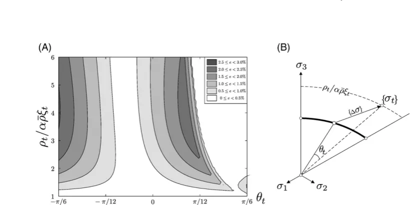
3.5. Stress return error analysis

The accuracy of the stress return algorithm was assessed for 1≤ρt/ (αρ̅(θt)ξt)≤6 and−π/6≤θt≤π/6. A Young's modulus of 100 MPa and a Poisson's ratio of 0.2 were used for the material's elastic properties.

α=−0.25 andρ̅e= 0.80 define the MR cone. A hydrostatic pressure ofξt=−1 MPa was used for all of the elastic trial stresses. In this analysis, the starting stress state was positioned on the yield surface at the shear meridian (θ= 0). The constitutive model was then subjected to an elastic strain increment corresponding to the elastic trial stress state, seeFig. 7(B). The return stress from this single strain increment was compared with the solution obtained by splitting the strain increment into 10,000 sub-increments.

The following error measure was used to assess the accuracy of the stress return algorithm

e=

ffiffiffiffiffiffiffiffiffiffiffiffiffiffiffiffiffiffiffiffiffiffiffiffiffiffiffiffiffiffiffiffiffiffiffiffiffiffiffiffiffiffiffiffiffiffiffiffiffiffiffiffiffiffiffiffiffiffiffiffiffiffiffiffiffi

ffσcpg−fσeggTffσcpg−fσegg

q

ffiffiffiffiffiffiffiffiffiffiffiffiffiffiffiffiffiffiffiffiffiffiffi

fσegTfσeg

q

;

ð65Þ

where {σe} is the “exact” stress return corresponding to the sub-incremented solution and {σcp} is the one-step analytical return. A

stress iso-error map is given inFig. 7(A). This analysis revealed a maximum error of 2.56%, corresponding to a trial stress on the extension meridian (θ=−π/6) atρt/(αρ̅ξt) = 4.1. Zero error appears along the locusθt= 0,ρt/(αρ̅ξt) = 1 toθt→−0.2160,ρt/(αρ̅ξt)→∞. Much of the trial area has an error of less than 0.5%. Larger errors are associated with trial stresses near the extension meridian and in the vicinity of the compression meridian return region. These are due to the increased tangential component of the trial stress increment. The non-smooth (stepped) region close toθt=π/12 is a consequence of the_finite grid size either side of the return region B_–C boundary.

4. Run time analysis

The run time of the single-step analytical BE return is compared with a conventional iterative BE stress return inFig. 8. The analysis considered trial stresses between 1≤ρt/(αρ̅ξt)≤6 and−π/6≤θt≤π/ 6. A Young's modulus of 100 MPa and a Poisson's ratio of 0.2 were again used for the material's elastic properties. Similarly,α=−0.25 andρ̅e= 0.8 define the MR cone and a hydrostatic pressure ofξt=

−1 MPa was used for all of the elastic trial stresses. The constitutive model was then subjected to a strain increment corresponding to the

elastic trial stress state, seeFig. 8(B). When returning to the corner or the apex, both the approaches (analytical and numerical BE) use the same single-step return discussed in the preceding sections. However, when returning onto the non-planar surface, the conventional (numerical) BE method requires multiple local iterations to obtain convergence. The number of iterations and the ratio of the numerical to analytical BE run times are presented inFig. 8(A). The analytical return demonstrates a 2.5–5.0 times speed-up over the iterative numerical method. The increase in time required for the iterative approach is due, in part, to repeatedly calculating thefirst and second derivatives of the yield function with respect to stress.

5. Finite-element performance

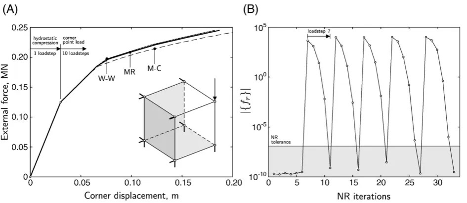
5.1. Single element test

A simple small-strainfinite-element analysis wasfirst undertaken to assess the constitutive model's performance within a general purpose 3D code. A single unit-cube 8-noded hexahedral element constrained on its lower horizontal, and two vertical, faces (seeFig. 9

(A)) was loaded under hydrostatic compression to−1 MPa in a single Fig. 8.(A) Run time comparison between conventional iterative backward Euler and the single-step analytical backward Euler stress return. (B) Geometric interpretation of the run time analysis.

(elastic) loadstep. Subsequently, a vertical point load of−0.12 MN was applied to the element's unconstrained top corner, via 10 equal loadsteps. A Young's modulus of 100 MPa and a Poisson's ratio of 0.2 were again used for the material's elastic properties. α=−0.25 andρ ̅e= 0.85 were adopted to define the MR, M–C and W–W cones. The load–displacement curves for the unconstrained corner in the vertical direction are shown inFig. 9(A).Fig. 9(B) illustrates the MR global convergence properties of the N–R iterations for each of the 11 loadsteps. Loadsteps 1–6 resulted in an elastic material response, whereas for loadsteps 7–11 the material behaviour was elasto-plastic. The latter demonstrate the asymptotic quadratic convergence of the N–R procedure. The following measure of (residual) out of balance force

jffrgj=

ffiffiffiffiffiffiffiffiffiffiffiffiffiffiffiffiffiffiffiffiffiffiffiffiffiffiffiffiffiffiffiffiffiffiffiffiffiffiffiffiffiffiffiffiffiffiffiffiffiffiffiffiffiffiffiffiffiffiffiffiffiffiffiffiffiffi

fffextg−ffintggTfffextg−ffintgg

q

ð66Þ

was used to assess convergence, where {fext} and {fint} are the external

and internal forces, respectively. |{fr}| for loadsteps 7–11 are given in

Table 2. The tolerance in steps (d) and (e) of the algorithm inTable 1

was set to 1 × 10−12_{, which corresponds to a N–R absolute tolerance}

of 1.2 × 10−7_N.

The results obtained from the three constitutive models are qualitatively similar, with the W–W and MR cones producing marginally stiffer responses when compared against the M–C simulation. A run time comparison for the single element test is presented inTable 3, where∑(NRit) is the total number of global N– R iterations, max (NRit) is the maximum number of iterations in any loadstep andt/tM–Cis the run time normalised with respect to the M–

C run time. The analytical BE MR approach (MRAn) was just 4.6% slower than the (over-simpli_fied) M_–C scheme. The analytical BE MR algorithm gave a 34.1% speed gain over the iterative BE MR approach (MRNum). More significantly, the Willam–Warnke (W–W)

formula-tion, which produced similar results to the MR cone, required a 25.9% increase in the run time.

5.2. Rigid strip footing analysis

A plane-strain incrementalfinite-element analysis of a 1 m wide rigid strip footing bearing onto a weightless soil was performed to assess the MR model's performance within a largerfinite-element problem. Due to symmetry, only one half of the problem was considered. The same_finite-element discretisation as presented in

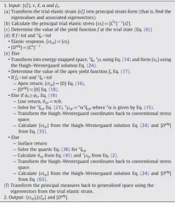
[6]was used, to allow comparisons to be made. The mesh had a depth and width of 5 m (Fig. 10). 135 eight-noded quadrilaterals, with reduced four-point quadrature, modelled the problem. The footing was assumed to be rigid and smooth with an imposed vertical displacement,u. Identical material properties as used in [6] were adopted here. These were: a Young's modulus of 10 GPa, Poisson's ratio of 0.48, cohesion,c, of 490 kPa, friction angle of 20° andρ ̅e= 0.8 Table 1

Pseudo code for the modified Reuleaux stress return algorithm. The tolerance (tol) in steps (d) and (e) is typically set to 1 × 10−12_.

1. Input: {εte},υ, E,αandρ̄e

(a) Transform the trial elastic strain{εte}into principal strain form (that is,find the

eigenvalues and associated eigenvectors). (b) Calculate the principal trial elastic stress {σt} = [Cˆe

]−1 {εte

}. (c) Determine the value of the yield functionfat the trial state (Eq.(6)) (d) Iffbtol andς_ξtbtol

•Elastic response, {σcp} = {σt} •[Dalg

] = [Ce ]−1 (e) Else

•Transform into energy-mapped space,ςξt,ςρtusing Eq.(14)and form {ςt} using the Haigh–Westergaard solution Eq.(24).

•Determine the value of the apex yield functionfaEq.(17).

•Iffabtol andςξtNtol

—Apex return, {σcp} = {0} Eq.(16). —[Dalg

] = [0] Eq.(18). •Else ifϕt≥ϕcrEq.(19)

—Line return,θcp=π/6.

—Solve forςξcpEq.(23),ςρcp=ςας_ξcpwhereς_{αis given by Eq.(15).}

—Transform the Haigh–Westergaard coordinates back to conventional stress space.

—Calculate {σcp} from the Haigh–Westergaard solution Eq.(24)and [Dalg

] from Eq.(33).

•Else

—Surface return

—Solve the quartic Eq.(38)forς_ξcp.

—Calculateθcpfrom Eq.(41)andς_{ρcpfrom Eq.(2).}

—Transform the Haigh–Westergaard coordinates back to conventional stress space.

—Calculate {σcp} from the Haigh–Westergaard solution Eq.(24)and [Dalg

] from Eq.(63).

(f) Transform the principal measures back to generalised space using the eigenvectors from the trial elastic strain.

2. Output: {σcp},{εcpe} and [Dalg].

Table 2

Residual out of balance force |{fr}| values for thefinite-element simulation. Normalised

residual out of balance force.

Iteration Loadstep

7 8 9 10 11

1 4.5576e + 03 9.818e + 03 9.7542e + 03 1.0232e + 04 1.0170e + 04 2 1.2707e + 03 1.3712e + 03 1.4912e + 03 3.7705e + 03 4.9317e + 03 3 2.6853e + 01 1.3767e + 01 3.0343e + 01 1.0539e + 02 5.4714e + 02 4 6.4122e−03 2.7541e−03 1.3201e−02 1.7086e−01 4.2900e−01 5 7.7098e−10 5.0493e−10 2.8944e−09 4.6539e−07 9.8050e−07

6 – – – 21973e−10 3.0211e−10

Table 3

Single 3Dfinite-element run time comparison.

M–C MRAn MRNum W–W

Σ(NRit) 36 33 33 32

max(NRit) 6 6 6 6

t/tM–C 1 1.046 1.387 1.305

(to coincide withρ ̅efor M–C). The material constants were common for the M–C, W–W and MR analyses.

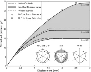
Fig. 11presents the normalised pressure_–displacement results for the three constitutive models. The M–C simulation gave a close agreement with the results presented by de Souza Neto et al.[6]. The normalised peak pressure approached the theoretical Prandtl solution (p/c= 14.8) to within 1.1%. Results for the MR cone usingρ ̅e= 0.51 andρ ̅e= 0.99 demonstrate the model's ability to provide solutions spanning between those provided by the M–C and D–P cones. With

ρ̅e= 0.8 the MR cone produced a stiffer response when compared against the M–C solution. The limit load tended top/c= 19.36. Results obtained from the W–W cone were quite similar; approaching a limit ofp/c= 20.69.

Table 4 gives run time comparisons for the three constitutive models at a vertical displacement of2 mm.nGpis the number of Gauss points which underwent plastic deformation by the end of the analysis.t/NRitgives the run time per global N–R iteration, whereas the ratio (tNRit)/(tM–CNRitM–C) gives this time normalised with respect

to the M_–C iteration time. The W_–W model required a 28.7% longer run time than the MR solution. The computational savings would be higher if a more efficient linear solver were used. Here the fi nite-element algorithm was coded in MATLAB m-script; using the backslash operator to solve the linear system. While the benefits of the MR formulation are already evident, a tuned pre-conditioned element-by-element Krylov solver[14], for example, would probably have reduced the CPU time associated with the linear solve, relative to the time spend on elasto-plastic stress integration. If this were the case, then the overall run time advantage of the MR model would be even greater.

6. Conclusion

The Drucker–Prager and Mohr–Coulomb models are amongst the most widely used simple pressure-sensitive perfect plasticity for-mulations in geomechanics. However, they fail to incorporate both the Lode angle and intermediate principal stress dependency typically seen in geomaterials. This omission has been shown by others to lead to errors infinite-element simulations[2]. Many constitutive models

now include such dependencies, but the algebraic expressions describing those formulations are relatively complex. This necessi-tates iterative numerical schemes to integrate the stresses. This can present a significant computational burden when undertaking detailed 2D and 3D analyses.

This paper presents the complete formulation for an associated perfect plasticity cone model which includes sensitivities to the Lode angle and the intermediate principal stress. It is based on a conical surface with modified Reuleaux deviatoric sections. The model allows the stresses to be integrated exactly when the previous and elastic trial stresses fall within the fan zones of the tensile apex or compression meridian (zones A and B respectively inFig. 3). Small integration errors associated with the backward Euler scheme may be introduced when returning to the curved surface (Fig. 7). For all regions, a single-step procedure is all that is required for the backward Euler approach.

The paper has demonstrated that the model offers an attractive alternative to the Drucker–Prager and Mohr–Coulomb models. Through material point and 2D plus 3Dfinite-element simulations, it has been shown that the computational advantages over a W_–W cone model are significant (Tables 3 and 4). The paper provides all the expressions for the consistent tangent appropriate for the three stress return regions on the yield surface. The model is simple to code (see

Table 1) and will be of interest to those simulating the behaviour of geomaterials and powders, where the response is governed by frictional slip.

Fig. 11.Normalised pressure–displacement for the rigid strip footing plane-strainfinite-element analysis.

Table 4

Rigid strip footing plane-strainfinite-element run time comparison.

M–C MRAn W–W

Σ(NRit) 6741 6075 6378

max(NRit) 12 10 11

nGp 473 470 470

t/tM–C 1 0.921 1.239

tNRM−C

it tM−CNRit

References

[1] J.P. Bardet, Lode dependences for isotropic pressure-sensitive elastoplastic materials, ASME, J. Appl. Mech. 57 (1990) 498–506.

[2] Z. Benz, M. Wehnert, P.A. Vermeer, A Lode angle dependent formulation of the Hardening Soil model, 12th IACMAG, 2008, pp. 653–660.

[3] S.K. Bhowmik, J.H. Long, A general formulation for the cross sections of yield surfaces in octahedral planes, in: G.N. Pande, J. Middleton (Eds.), Numenta 90, 1990, pp. 795–803.

[4] J. Clausen, L. Damkilde, L. Andersen, Efficient return algorithms for associated plasticity with multiple yield planes, Int. J. Numer. Meth. Engng. 66 (2006) 1036–1059.

[5] R.S. Crouch, H. Askes, T. Li, Analytical CPP in energy-mapped stress space: application to a modified Drucker–Prager yield surface, Comput. Meth. Appl. Mech. Engrg. 198 (5–8) (2009) 853–859.

[6] E.A. de Souza Neto, D. Perić, D.R.J. Owen, Computational Methods for Plasticity: Theory and Applications, John Wiley & Sons Ltd, , 2008.

[7] D.V. Griffiths, Failure criteria interpretation based on Mohr–Coulomb friction, ASCE, J. Geotech. Engrg. 116 (6) (1990) 986–999.

[8] P.V. Lade, J.M. Duncan, Cubical triaxial tests on cohesionless soil, J. Soil Mech. Found. Div. ASCE (1973) 193–812.

[9] FC Moon, Franz Reuleaux: Contributions to 19th C. kinematics and theory of machines, Tech. report, Cornell Library Technical Reports and Papers, 2002. [10] J. Podgorski, General failure criterion for isotropic media, ASCE, J. Engrg. Mech. 111 (2)

(1985) 188–201.

[11] F. Reuleaux, The Kinematics of Machinery: Outlines of a Theory of Machines, Macmillan and Co, London, 1876.

[12] A. Sayão, Y.P. Vaid, Effect of intermediate principal stress on the deformation response of sand, Can. Geotech. J. 33 (1996) 822–828.

[13] J.C. Simo, T.J.R. Hughes, Computational Inelasticity, Springer, New York, 1998. [14] I.M. Smith, A general purpose system forfinite element analyses in parallel, Engrg.

Comput. 17 (1) (2000) 75–91.

[15] M. Vrh, M. Halilovič, B.Štok, Improved explicit integration in plasticity, Int. J. Numer. Meth. Engng. 81 (2010) 910–938.

[16] K.J. Willam and E.P. Warnke, Constitutive model for the triaxial behaviour of concrete, Proceedings of the May 17–19 1974, International Association of Bridge and Structural Engineers Seminar on Concrete Structures Subjected to Triaxial Stresses, held at Bergamo Italy, 1974.