Shakedown analysis of a composite cylinder with a cross-hole

Shakedown Analysis of a Composite Cylinder with a Cross-hole

Haofeng Chen*, Weihang Chen, Tianbai Li, James Ure

Department of Mechanical Engineering, University of Strathclyde, Glasgow, G1 1XJ, UK

Abstract: In this study, both the lower and upper bound shakedown limits of a closed-end composite cylinder with or without a cross-hole subject to constant internal pressure and a cyclic thermal gradient are calculated by the Linear Matching Method (LMM). Convergence for upper and lower bound shakedown limits of the composite cylinders is sought and shakedown limit interaction diagrams of the numerical applications identifying the regions of reverse plasticity limit and ratchet limit are presented. The effects of temperature-dependent yield stress, material discontinuities, composite cylinder thickness and the existence of the cross-hole on the shakedown limits are discussed for different geometry parameters. Finally, a safety shakedown envelope is created by formulating the shakedown limit results of different composite materials and cylinder thickness ratios with different cross-hole sizes.

Keywords: lower and upper bound, shakedown, linear matching method, composite cylinder

1 Introduction

Materials have largely been kept responsible for performance improvements in many areas of structures technology. The continuous development of computational structures technology and the advanced composite materials have improved structural performance, reduced operational risk, and shortened production time [1]. On the other hand, one of the most important reasons for using composite materials is the reduction of weight [2].

With the achievements in aerospace industry, the strength-to-weight ratio of engineering components has become a very important design criterion since a high strength-to-weight ratio results in a better performance and greater shear strength. The lower weight results in lower fuel consumption and emissions.

*

Corresponding author.

Email: haofeng.chen@strath.ac.uk

Strength-to-weight ratio can increase in case the elastic limit of materials is surpassed and the allowable accumulated plastic strain constraints are assigned. In this way the design of composite pressure cylinder subjected to cyclic mechanical and thermal loads can be achieved. The investigations of the elastic and elastic-plastic behaviour of a uniform cylinder under constant internal pressure and cyclic thermal loads with a cross-hole are presented by the well-known Bree-like diagram in [3] and [4].

The local stress concentration is redistributed around the material boundaries for composite cylinders under cyclic thermal loads. It changes the fatigue life and elastic shakedown limits of the cylinder. The elastic shakedown limit is the highest cyclical load that shakes down to an elastic response in the first few cycles of load. When the elastic shakedown limit is exceeded, the cylinder may experience either plastic shakedown or ratcheting. In many applications, it is allowable for a structure to be within the elastic shakedown limit, but plastic shakedown or alternating plasticity, under which a local low cycle fatigue failure mode occurs, and ratcheting that ultimately leads to incremental plastic collapse, are not permitted. Consequently the shakedown limit is a particularly important design condition to the pressure cylinder. The elastic-plastic behaviour of the structure needs to be well comprehended while using this design condition since the elastic-plastic reaction is load path dependent and most commonly simulated by an incremental Finite Element Analysis (FEA). This allows investigation of any type of load cycle but also requires detailed load history and involves significant computer effort.

To avoid such difficulties, direct methods are incorporated into finite element analysis in order to evaluate the shakedown limit. The model’s material is considered to be elastic perfectly plastic, and the load domain including all the possible load paths eliminates the necessity to know the load history particularities in detail. Such methods include mathematical programming methods [5-7], the Generalized Local Stress Strain (GLOSS) r-node method [8], the Elastic Compensation Method (ECM) [9,10], and the Linear Matching Method (LMM) [11-14]. Among these direct methods, the LMM is considered to be the most adaptable method to practical engineering applications that involve complex cyclic thermo-mechanical load conditions. Other direct methods require specific programs that are not available or supported commercially, or have difficulties to effectively analyze complex engineering structures. The stable and accurate results of the LMM on shakedown analysis have been confirmed in many industrial applications, including the problem of the defective pipeline [11] and a super heater outlet penetration tube plate [15].

materials and thickness ratios with and without cross-holes. Three cross-hole sizes are considered, all relatively small in comparison with the other cylinder dimensions. The objective of the investigation is to formulate a safety shakedown limit region for industrial purposes using the calculated shakedown limit results of different composite material ratio and cylinder thickness ratio with different cross-hole sizes.

2 Numerical Procedures

The basic assumption and yield condition of the analysis of shakedown is provided in [16]. A detailed mathematical derivation of shakedown analysis is given in [17]. For solving problems of high temperature effects, the yield stress of the material is considered to be temperature-dependent. This dependence is implemented at Gauss points and related to every loading vertex of the loading domain. Let a body subjected to a cyclic history of varying temperature

λθ

(xi,t) within the volume

of the structure and surface loads λP_i(x_i,t)acting over part of the structure’s surface

S

_{T be} considered. The variation is considered to be over a typical cycle

0

≤

t

≤

Δ

t

. Here

λ

denotes a load parameter, allowing a whole class of loading histories to be taken into account. On the remainder of the surface S , denoted as S_u, the displacement is u_i =0. Corresponding to these loading histories, a linear elastic solution history is obtained:

P ij ij

ij

λ

σ

λ

σ

σ

λ

θ

ˆ

ˆ

ˆ

=

+

(1)

where

σ

ˆ_ijθ and

σ

ˆ_ijP are the elastic solutions corresponding to

θ

(

x

_i

,

t

)

and

P

_i

(

x

_i

,

t

)

, respectively. For shakedown cyclic problems, the cyclic stress history during a typical cycle

0

≤

t

≤

Δ

t

, irrespective of material properties is given by

σ

ij

(

x

i

,

t

)

=

λ

σ

ˆ

ij

(

x

i

,

t

)

+

ρ

ij

(

x

i

)

(2)

where

ρ

_ij denotes a constant residual stress field in equilibrium with zero surface tractions on

S

_T, and corresponds to the residual state of stress at the beginning and the end of the cycle.

2.1 Upper Bound Procedure

Koiter's theorem [18] states: For all Kinematically Admissible (KA) strain rate histories

∫ ∫

∫ ∫

∫ ∫

= =T

V c ij c ij c

ij T

V c

ij T

V ij

UB xt dVdt D dVdt dVdt

0 0

0

) ( )

, (

ˆ

ε

ε

σ

ε

σ

λ

& & & (3)

where

σ

_ijc denotes a state associated with

ε

&_ijc (all strain rate histories that accumulate over a cycle) at yield, then

λ

UB

≥

λ

s, where

λ

s is the exact shakedown limit. Koiter's theorem is also referred to as the upper bound shakedown theorem.

Theory [11] shows the form ( iUB f UB

λ

λ

≤ ) of the upper bound theorem that allows the LMM to be displayed as a programming method. [17] demonstrates that the yield condition and the linear material provide the same stress for strain rate history at an initial KA

ε

&

iji . As a result the matching condition is:

pi ij Li ij

σ

σ

=

(4) where

σ

ijpi is the associated stress at yield .

For the von Mises yield condition, matching condition (4) becomes:

i y

ε

σ

μ

&

3 2 =

(5)

where

ε

&

denotes the von Mises effective strain rate and

μ

denotes shear modulus. The upper bound multiplier can be obtained by a single iterationthat begins with the evaluation of a varying shear modulus

μ

by matching the stress due to the linear model and the yield condition at the strain rate

ε

&

iji yielded by the previous iteration. Each step in iteration provides both a kinematically admissible strain rate history and an equilibrium distribution of residual stress, while upper bounds are generated such that they converge to the minimum upper bound.

2.2 Lower Bound Procedure

Melan's theorem [19] states: If a time constant residual stress field

ρ

exists such that superposition with induced elastic stresses

λ

LB

σ

ˆij(x,t)forms a safe state of stress everywhere in the

f

(

λ

LB

σ

ˆ

ij

(

x

i

,

t

)

+

ρ

ij

(

x

i

))

≤

0

(6a) then (6b) Melan's theorem can also be referred to as lower bound shakedown theorem or static shakedown theorem. On the basis of Melan's lower bound shakedown theorem, a lower bound of shakedown limit can be constructed using the same procedure by maximizing the lower bound load parameter λ_LB under the condition where for any potentially active load/temperature path, the stresses resulting from the superposition of this constant residual stress field

ρ

ij with the thermal-mechanical elastic stress λ_LBσˆ nowhere will violate the temperature-dependent yield condition. _ij Hence, as the above upper bound iterative process provides a sequence of residual stress fields, it is possible to evaluate a lower bound at each step of the iteration by scaling the elastic solution so that

ij ij LB

σ

ρ

λ

ˆ + satisfies the yield condition everywhere. The lower bound of shakedown limit

multiplier can be written as:

λ

s_LB

=

max

λ

_LB

2.3 Iteration Steps of LMM Shakedown Analysis

A very significant advantage of the method comes from the ability to use standard commercial finite element codes which have the facility to allow the user to define the material behaviour. This has been done within the code ABAQUS with user subroutine UMAT. Essentially, ABAQUS carries out a conventional step-by-step analysis and, through the use of the user subroutine, each increment is reinterpreted in terms of an iteration of the method. At each increment, the user subroutine UMAT allows a dynamic prescription of the Jacobian which defines the relationship between increments of stress and strain. Fig. 1 presents a flow chart showing the i+1 iteration steps in ABAQUS for estimating the shakedown limit using the upper and lower bound theorem. A detailed iteration for lower bound and upper bound shakedown limit is given in [16].

3 Composite Cylinder Geometry

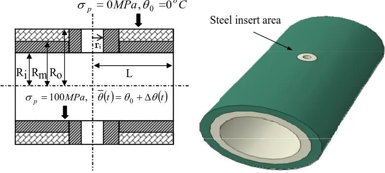
The geometrical shape and the material properties of the composite cylinder with a cross-hole are as shown in Fig. 2 and Table 1, respectively. The composite thick cylinder has an inner layer of steel and an outer layer of aluminum. Ri, Rm, Ro are the inner radius, middle radius, and outer radius of the composite cylinder, respectively.

The area surrounding the hole, which can be an instrumentation tapping or a port for the fluid entry or exit, is expected to be the most critical region since this is a structure discontinuity causing the rise of the local stress concentration. To improve the mechanical performance of this critical region, the material surrounding the hole is selected to be the same high performance steel as the inner portion of the composite cylinder. The thickness of the cylindrical shape steel insert is equal to the half thickness of the composite cylinder

2

i o R

R −

.

The shakedown results are obtained for three different radius ratios:Ro Ri =1.5,1.75,2.0. Three

cross-hole radius ratios are also modelled: r_i R_i =0.1,0.2,0.3. The maximum radius ratios i i R r

defined in this paper meet the requirement of ASME B&PV Code Section VIII Division 2, in which the limitation of

i i R r

should be less or equal to 1/2 for perforated cylindrical shells [20]. The

analysis is performed forthree composite material ratios: ,1,3 3 1

=

A s V

V , where Vsand VA stand for the volume of steel and aluminum, respectively. For better comparison of results, in all the cases the inner radius is chosen to be R_i =300mm while length is

L

=

900

mm

.

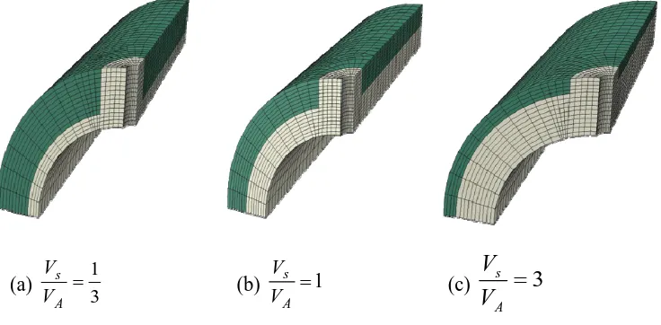
4 Finite Element Modelling

The composite cylinders are analyzed using ABAQUS type C3D20R 20 node quadratic brick elements with reduced integration scheme. The composite cylinders with cross-holes have three planes of symmetry. Hence, to minimize the size of the model, these symmetry boundary conditions are applied to a quarter section of the model. A closer 3D view of a composite cylinder with cross-hole is shown in Fig. 3. The main cylinder bore and the cross-hole bore are under constant internal pressure. The cut end of the cylinder is constrained in order to keep the plane section plane during loading. The closed-end boundary condition is achieved by applying uniform axial thrust to the end of the cylinder. The holes are assumed to have open-ended boundary condition. The applied cyclic thermal loading is produced by assuming that the outside surface of the cylinder is at ambient temperature while the internal surface temperature is fluctuating from ambient to higher values. Three thermal stress extremes are adopted for this cyclic load history:

- Secondly, a thermal stress occurring at the highest uniform temperature is applied due to the material mismatch. This thermal stress is adopted knowing that thermal expansions between the steel and aluminum are significantly different;

- Finally, a zero thermal stress field is selected to simulate a uniform ambient temperature for the whole cylinder.

When the ambient temperature

θ

0 remains at C

o

0 , the magnitudes of the maximum von Mises effective thermo elastic stresses for the above thermal loading extremes can be determined by the maximum temperature differenceΔ

θ

between the inner surface and outer surface of the composite cylinder. Hence these thermal and mechanical load path extremes can be characterized by the maximum temperature differenceΔ

θ

and the internal pressure

σ

p . The reference constant elastic mechanical stress can be calculated by the internal pressure p p y 100MPa

aluminum

0= =

=σ σ

σ while

the reference temperature difference Δ

θ

=Δ

θ

₀ =100oCdetermines the reference cyclic thermal elastic stresses. When the temperature-dependent yield stress

σ

Y

(

T

)

is adopted, the actual load

factor is updated in an iterative way during the calculation. The adopted temperature-dependent yield stress is given in equation (7) for steel and presented in Table 2 for aluminum:

σ

_Y

(

T

)

=

σ

_Y0

−

0

.

4

(

MPa

/

°

C

)

×

T

₍₇₎

5 Results and Discussions

5.1 Upper and Lower Bound Results with Temperature Dependent and Independent Yield Stresses

Based upon the kinematic theorem of Koiter [18], the LMM procedure has proved to produce highly accurate upper bound [11] and lower bound shakedown limits [16]. The converged values of both upper and lower bounds shakedown limits for the composite cylinder are shown in Fig. 4 where material ratios, cylinder and cross-hole radius ratios are =1

A s V V

, =1.75 i o R R

, =0.1 i i R r

the ratchet limit BC/ B*C. This is known as “ratcheting” or “incremental plastic collapse”. The point C corresponds to the limit load for the applied mechanical load. There are significant differences between the reverse plasticity limit A*B* adopting temperature-dependent yield stress and the reverse plasticity limit AB considering temperature-independent yield stress. Hence it is important to adopt temperature-dependent yield stress for a structure assessment under high temperature variations. However, in order to simplify the calculations, the temperature-independent yield stress can be adopted when the variation of operating temperature approaches to zero or the temperature varies within a limited range. The temperature effects on the yield stress may be ignored in such conditions.

Fig. 4b shows typical upper and lower bound sequences converging after 70 iterations for load point A (Fig. 4a) considering temperature-independent yield stress, and for load point A*(Fig. 4a) considering temperature-dependent yield stress. It can be observed that both the upper bound and lower bound converge to the exact shakedown limit proving that LMM produces highly accurate upper bound and lower bound shakedown limit results. For the simplification of discussion, the results in the next section only show the upper bound shakedown limit for the temperature-independent yield stress.

In order to verify the accuracy of the LMM, four load cases (labelled D, E, F and G in Fig.4a) with cyclic thermal loads of 1.25

0

= Δ

Δ θ

θ _,

35 . 1

0 = Δ

Δ

θ

θ _,

7 . 0

0 = Δ

Δ

θ

θ _and

7 . 0

0 = Δ

Δ

θ

θ _{respectively, have been}

performed using ABAQUS step-by-step analyses. The plastic strain histories representing the maximum plastic strain range for the cyclic loading cases D, E, F and G are shown in Fig.5. Load cases D (Fig.5a) and F (Fig.5b) exhibit shakedown mechanism as the calculated equivalent plastic strain stop changing after 2 load cycles. The calculated equivalent plastic strain for the load case E (Fig.5a) converges to a closed cycle after about 9 load cycles showing a reverse plasticity mechanism, and the load case G (Fig.5b) shows a strong ratcheting mechanism, with the equivalent plastic strain increasing at every cycle. Thus, the results in Fig.5 obtained using ABAQUS step-by-step analysis confirm the accuracy of the predicted shakedown limits by the LMM. Further benefits of the LMM can be found considering the computing time necessary to generate the shakedown curves. The time that the LMM needed to generate the points on the ratcheting boundary was less than 10% of that needed for the above four load cases to complete using the ABAQUS step-by-step analyse.

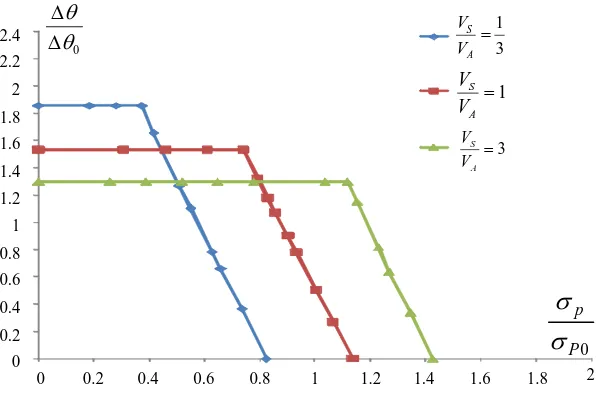
The shakedown limit interaction curves of a composite cylinder with varying material ratio configurations (Fig. 3) are presented in Fig. 6. The applied pressure in X-axis is normalized with respect to the reference internal pressure while the thermal load in Y-axis is normalized by using the reference temperature differenceΔθ =Δθ₀ =100oC.

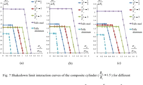
Fig. 6 shows that the limit load of the composite cylinder reduces when the volume of steel material is decreasing, whereas the reverse plasticity limit is increased with smaller

A s

V V

. The reduction in the limit load is approximately in proportion to the loss of steel material. The increasing reverse plasticity limit is due to the difference in thermal conductivities of the steel and aluminum. As the volume of aluminum increases, a larger proportion of the cylinder will have larger thermal conductivity, which leads to a lower thermal elastic stress range. Hence, when the volume of aluminum increases the reverse plasticity limit increases. Shakedown limit interaction curves of the composite cylinder ( =1.5

i o R R

) with cross-hole for different composite material ratios and different hole ratios are presented in Fig. 7 which shows that with the addition of a cross-hole, the general trend of the shakedown curves is similar to Fig. 6. Both figures show a decreasing limit load and increasing reverse plasticity limit for decreasing volume of steel. It is worth noting that for the pure material cases, the reverse plastic limit is determined by the maximum thermal stress due to the temperature gradient while the reverse plastic limit for the composite material is defined by the maximum thermal stress due to the material mismatch. The addition of a hole gives rise to a local stress concentration. This is shown to have little effect on the limit load for any material configuration when the hole diameter is small. A detailed discussion of the effects of the hole diameter is given in section 5.3.

5.3 Effect of the Hole Diameter

Cross-holes in composite cylinders are structural discontinuities which increase elastic stress due to local stress concentration. The influence of cross-hole size, r_i R_i =0.1,0.2,0.3on the shakedown limit interaction curve is shown in Fig. 8 for different material ratio configurations.

Fig. 8a shows that for a material ratio of

3 1

, the addition of a hole has a large impact on the reverse plasticity limit, which demonstrates the dominance of this stress raiser to the mechanism. The addition of a hole is shown to have negligible effect on the limit load. When the material ratio

3 1

= A s V V

lower yield stress. The introduction of a hole has much less effect on the limit load than this small material ratio.

Fig. 8b demonstrates that for a material ratio of 1, the addition of a hole has a sizable effect on the reverse plasticity limit, but impacts the limit load less significantly than Fig. 8c for a material ratio of 3. This is because when the material ratio reduces to 1, the stress concentration from the hole becomes comparable with the stress concentration due to the material mismatch. When the size of hole increases, both the limit load and reverse plasticity limit decreases.

Fig. 8c shows that for a material ratio of 3, the addition of a hole has little effect on the value of reverse plasticity limit, but causes a reduction in the limit load. The reduction in material by an increasing hole diameter is the cause of the reduction in limit load. There is little effect of the hole size on the reverse plasticity limit due to the dominance of the material boundary stress raiser, which has little interaction with the stress concentration caused by the hole.

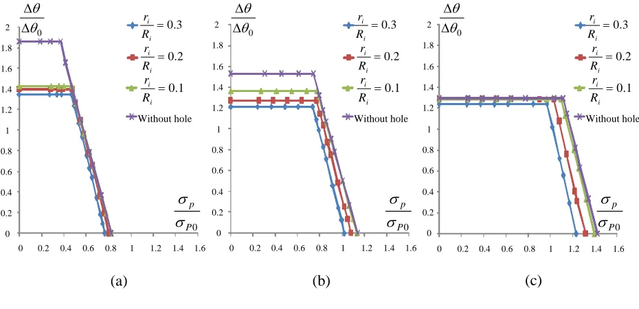
5.4 Effect of the Composite Cylinder Thickness

Fig. 9 presents the effects of the radius ratio i o R R

on the shakedown limit interaction curve. Three different relative thicknesses R_o R_i=1.5,1.75,2.0 of the composite cylinder with a fixed material ratio of 1 were analyzed.

Increasing this radius ratio greatly increases the limit load and reduces the reverse plasticity limit. The increase in limit load is an obvious result, as effectively the thickness of the pipe is increased for the same inner radius. The reduction in the reverse plasticity limit is caused by the increased thickness of steel. This increase in thickness (which causes greater conductive temperatures in the steel) results in higher thermal stresses at the material boundary.

5.5 Formulated Shakedown Limit Design Region

An elastic shakedown limit formulation of the composite cylinder is made for the safety of engineering design. The elastic shakedown design regions of composite cylinders are shown in Fig. 10, whereΔθRL is the design temperature range corresponding to the reverse plasticity limit, PRL is the design internal pressure representing the limit load and S_RLis the design slope of the ratchet limit curve. In order to simplify the formulation,ΔθRL,PRLand SRLare assumed to be the product of three independent functions _⎟⎟

⎠ ⎞ ⎜⎜ ⎝ ⎛

i i

R r

f1 , ⎟⎟

⎠ ⎞ ⎜⎜ ⎝ ⎛

A S

V V

f_{2 , ⎟⎟}

⎠ ⎞ ⎜⎜ ⎝ ⎛

i o

R R

f_{3 ; ⎟⎟}

⎠ ⎞ ⎜⎜ ⎝ ⎛

i i

R r

g_{1 , ⎟⎟} ⎠ ⎞ ⎜⎜ ⎝ ⎛

A S

V V

g_{2 , ⎟⎟} ⎠ ⎞ ⎜⎜ ⎝ ⎛

i o

R R

g_{3 ,and ⎟⎟} ⎠ ⎞ ⎜⎜ ⎝ ⎛

i i

R r

h1 , ⎟⎟ ⎠ ⎞ ⎜⎜ ⎝ ⎛

A S

⎟⎟ ⎠ ⎞ ⎜⎜ ⎝ ⎛ i o R R

h3 respectively. The X direction is the applied pressure PRL and the Y direction is the applied temperature differenceΔθRL. Therefore, the design shakedown limits are formulated as

(8)

(9)

(10)

Where _⎟⎟

⎠ ⎞ ⎜⎜ ⎝ ⎛ i i R r

f_{1 , ⎟⎟}

⎠ ⎞ ⎜⎜ ⎝ ⎛ A S V V

f2 , ⎟⎟

⎠ ⎞ ⎜⎜ ⎝ ⎛ i o R R

f3 , are the influence functions for the design temperature range

corresponding to the reverse plasticity limit, _⎟⎟

⎠ ⎞ ⎜⎜ ⎝ ⎛ i i R r

g_{1 , ⎟⎟} ⎠ ⎞ ⎜⎜ ⎝ ⎛ A S V V

g_{2 , ⎟⎟} ⎠ ⎞ ⎜⎜ ⎝ ⎛ i o R R

g_{3 are the influence functions}

for the design internal pressure representing the limit load, and _⎟⎟

⎠ ⎞ ⎜⎜ ⎝ ⎛ i i R r

h_{1 , ⎟⎟}

⎠ ⎞ ⎜⎜ ⎝ ⎛ A S V V

h_{2 , ⎟⎟} ⎠ ⎞ ⎜⎜ ⎝ ⎛ i o R R

h_{3 are the}

influence functions for the design slope of the ratchet limit curve. i i R r , A S V V and i o R R

stand for the cross-hole ratio, steel to aluminum ratio and thickness ratio, respectively.

L

θ

Δ , PLand SL are constants standing for the calculated reverse plasticity limit, the limit

internal pressure and the slope of the ratchet limit curve in case of =1.5 i o

R R

, =1 A S

V V

without a cross-hole, where,

Δ

θ

L =153oC (11a) P_L =113.8MPa (11b) S_L =3.873οC/MPa (11c) In order to find these influence functions, the obtained reverse plasticity limits, limit internal pressure and the slope of the ratchet limit curve are replotted in graphs of functions f, g and h against i i R r , A S V V and i o R R

respectively as shown in Fig. 11, Fig. 12 and Fig.13. Trend lines are fitted to the data obtained from the shakedown limit results of different composite material ratio and cylinder thickness ratio with different cross-hole sizes to show the influence function.

⎟⎟ ⎠ ⎞ ⎜⎜ ⎝ ⎛ ⎟⎟ ⎠ ⎞ ⎜⎜ ⎝ ⎛ ⎟⎟ ⎠ ⎞ ⎜⎜ ⎝ ⎛ = i o A S i i L RL R R g V V g R r g P

P _{1 2 3}

⎟⎟ ⎠ ⎞ ⎜⎜ ⎝ ⎛ ⎟⎟ ⎠ ⎞ ⎜⎜ ⎝ ⎛ ⎟⎟ ⎠ ⎞ ⎜⎜ ⎝ ⎛ Δ = Δ i o A S i i L RL R R f V V f R r

f_{1 2 3}

θ θ ⎟⎟ ⎠ ⎞ ⎜⎜ ⎝ ⎛ ⎟⎟ ⎠ ⎞ ⎜⎜ ⎝ ⎛ ⎟⎟ ⎠ ⎞ ⎜⎜ ⎝ ⎛ = i o A S i i L RL R R h V V h R r h S

Equations (12a-12c), (13a-13c) and (14a-14c) are the obtained influence functions for the design temperature range corresponding to the reverse plasticity limit, the design internal pressure representing the limit load, and the design slope of the ratchet limit curve, respectively. OnceΔ

θ

RL,

RL

P andSRL, are defined, a safety shakedown envelope is created as shown in Fig. 10.

⎪ ⎪ ⎪ ⎪ ⎩ ⎪⎪ ⎪ ⎪ ⎨ ⎧ < ≤ < ≤ + ⎟⎟ ⎠ ⎞ ⎜⎜ ⎝ ⎛ − = = ⎟⎟ ⎠ ⎞ ⎜⎜ ⎝ ⎛ ) 7 . 0 3 . 0 ( 803 . 0 ) 3 . 0 1 . 0 ( 926 . 0 411 . 0 ) 0 ( 1 1 i i i i i i i i i i R r R r R r R r R r f (12a) ⎪ ⎪ ⎩ ⎪ ⎪ ⎨ ⎧ ≤ ≤ + ⎟⎟ ⎠ ⎞ ⎜⎜ ⎝ ⎛ − ⎟⎟ ⎠ ⎞ ⎜⎜ ⎝ ⎛ = ⎟⎟ ⎠ ⎞ ⎜⎜ ⎝ ⎛ ) ( 495 . 1 ) 3 3 1 ( 072 . 1 087 . 0 015 . 0 ) aluminum ( 659 . 0 2 2 steel pure V V V V V V pure V V f A S A S A S A S (12b) ) 25 . 2 5 . 1 ( 989 . 1 659 . 0

3 ⎟⎟+ ≤ ≤

⎠ ⎞ ⎜⎜ ⎝ ⎛ − = ⎟⎟ ⎠ ⎞ ⎜⎜ ⎝ ⎛ i o i o i o R R R R R R

f _(12c)

⎪ ⎪ ⎪ ⎪ ⎩ ⎪ ⎪ ⎪ ⎪ ⎨ ⎧ < ≤ + ⎟⎟ ⎠ ⎞ ⎜⎜ ⎝ ⎛ − < ≤ + ⎟⎟ ⎠ ⎞ ⎜⎜ ⎝ ⎛ − = = ⎟⎟ ⎠ ⎞ ⎜⎜ ⎝ ⎛ ) 7 . 0 3 . 0 ( 156 . 1 872 . 0 ) 3 . 0 1 . 0 ( 043 . 1 494 . 0 ) 0 ( 1 1 i i i i i i i i i i i i R r R r R r R r R r R r g (13a) ⎪ ⎪ ⎩ ⎪ ⎪ ⎨ ⎧ ≤ ≤ + ⎟⎟ ⎠ ⎞ ⎜⎜ ⎝ ⎛ = ⎟⎟ ⎠ ⎞ ⎜⎜ ⎝ ⎛ ) ( 433 . 1 ) 3 3 1 ( 827 . 0 173 . 0 ) aluminum ( 402 . 0 2 steel pure V V V V pure V V g A S A S A S (13b) ) 25 . 2 5 . 1 ( 84 . 0 227 . 1

3 ⎟⎟− ≤ ≤

⎠ ⎞ ⎜⎜ ⎝ ⎛ = ⎟⎟ ⎠ ⎞ ⎜⎜ ⎝ ⎛ i o i o i o R R R R R R

⎪ ⎪ ⎪ ⎪ ⎩ ⎪ ⎪ ⎪ ⎪ ⎨ ⎧ < ≤ + ⎟⎟ ⎠ ⎞ ⎜⎜ ⎝ ⎛ − < ≤ + ⎟⎟ ⎠ ⎞ ⎜⎜ ⎝ ⎛ − = = ⎟⎟ ⎠ ⎞ ⎜⎜ ⎝ ⎛ ) 7 . 0 3 . 0 ( 855 . 0 058 . 0 ) 3 . 0 1 . 0 ( 061 . 1 743 . 0 ) 0 ( 1 1 i i i i i i i i i i i i R r R r R r R r R r R r h (14a) ⎪ ⎪ ⎩ ⎪ ⎪ ⎨ ⎧ ≤ ≤ + ⎟⎟ ⎠ ⎞ ⎜⎜ ⎝ ⎛ = ⎟⎟ ⎠ ⎞ ⎜⎜ ⎝ ⎛ ) ( 324 . 1 ) 3 3 1 ( 971 . 0 029 . 0 ) aluminum ( 988 . 1 2 steel pure V V V V pure V V h A S A S A S (14b)

)

25

.

2

5

.

1

(

165

.

2

777

.

0

3

⎟⎟

+

≤

≤

⎠

⎞

⎜⎜

⎝

⎛

−

=

⎟⎟

⎠

⎞

⎜⎜

⎝

⎛

i o i o i o

R

R

R

R

R

R

h

_(14c)

6 Conclusion

The Linear Matching Method has been verified by step-by-step analyses, showing that it gives very accurate shakedown limits for the composite cylinder with a cross hole. The result obtained using the LMM for the composite cylinder without a cross-hole shows that the limit load decreases with the reduction of the steel material, whereas the reverse plasticity limit increases with the decreasing volume of steel. With the cross-hole addition, the general trend of the shakedown curves is similar to the one without a cross-hole - a decreasing limit load and increasing reverse plasticity limit for decreasing volume of steel. For steel to aluminium ratio =3

A s V V

, the existence of a hole has little effect on the value of reverse plasticity limit, but it causes a reduction in the limit load. For material ratio of 1, the existence of a hole has a sizable effect on the reverse plasticity limit, but impacts the limit load less significantly than for a material ratio of 3. For a material ratio

3 1 = A s V V , the hole is shown to have negligible effect on the limit load. This implies that the size of the cross-hole raised the local stress concentration which will influence the fatigue life but will not greatly affect the global response when the limit load is determined by the low yield stress of the dominant aluminium material. Increasing the cylinder radius ratio

i o R R

shakedown limit results of different composite material and cylinder thickness ratios with different cross-hole sizes.

Acknowledgements

The authors gratefully acknowledge the support of the Engineering and Physical Sciences Research Council of the United Kingdom, and the University of Strathclyde during the course of this work.

References

1. Noor, Ahmed K., 2000, “Structures technology for future aerospace systems,” Computers and Structures, 74, pp.507-519

2. Thuis, H.G.S.J., & Biemans, C., 1997,“Design fabrication and testing of a composite bracket for aerospace applications,”Composite Structures, 38, pp. 91-98

3. Makulsawatudom, P., Mackenzie, D., and Hamiton, R., 2004, “Shakedown behaviour of thick cylindrical vessels with cross-holes,” Proc. Instn Mech. Engrs, 218, Part E: J. Process Mechanical Engineering

4. Camilleri, D., Mackemzie, D., Hamilton, R., 2009, “Shakedown of a Thick Cylinder With a Radial Crosshole,” Journal of Pressure Vessel Technology 131(1), 011203-1

5. Liu YH, Carvelli V, Maier G., 1997, “Integrity assessment of defective pressurized pipelines by direct simplified methods”. International Journal of Pressure Vessels and Piping, 74, pp.49–57 6. Vu, D.K., Yan, A.M., Nguyen-Dang, H., 2004, “A primal–dual algorithm for shakedown

analysis of structures”. Comput. Methods Appl. Mech. Eng, 193, pp.4663–4674

7. Staat M., Heitzer M., 2001, “LISA a European Project for FEM-based Limit and Shakedown Analysis”, Nuclear Engineering and Design, 206, pp.151–166.

8. Seshadri, R., 1995, “Inelastic Evaluation of Mechanical and Structural components Using the Generalized Local Stress Strain Method of Analysis”, Nucl. Eng. Des., 153, pp.287-303

9. Mackenzie, D., Boyle, J. T., Hamilton, and R. & Shi, J., 1996, “Elastic compensation method in shell-based design by analysis,” Proceedings of the 1996 ASME Pressure Vessels and Piping Conference, 338, pp. 203-208

11.Chen, H.F., Ponter ARS., 2001, “Shakedown and limit analyses for 3-D structures using the Linear Matching Method”, International Journal of Pressure Vessels and Piping , 78, pp.443– 451.

12.Chen, H.F. and Ponter, A.R.S., 2001, “A Method for the Evaluation of a Ratchet Limit and the Amplitude of Plastic Strain for Bodies Subjected to Cyclic Loading”, European Journal of Mechanics, A/Solids, 20 (4), pp.555-571

13.Chen, H.F., Ponter, A.R.S and Ainsworth, R.A., 2006, “The Linear Matching Method applied to the High Temperature Life Integrity of Structures, Part 1: Assessments involving Constant Residual Stress Fields”, International Journal of Pressure Vessels and Piping, 83(2), pp.123-135 14.Chen, H.F., Ponter, A.R.S and Ainsworth, R. A., 2006, “The Linear Matching Method applied

to the High Temperature Life Integrity of Structures, Part 2: Assessments beyond shakedown involving Changing Residual Stress Fields”, International Journal of Pressure Vessels and Piping, 83(2), pp.136-147

15.Chen, H.F. & Ponter, A.R.S., 2009, “Structural integrity assessment of super heater outlet penetration tube plate,” International Journal of Pressure Vessels and Piping, 86, 412–419

16.Chen, H.F., 2010, “Lower and Upper Bound Shakedown Analysis of structures With Temperature-Dependent Yield Stress”, Journal of Pressure Vessel Technology, 132(1), 011202-1

17.Ponter, A.R.S. & Chen, H.F., 2001, “A minimum theorem for cyclic load in excess of shakedown, with application to the evaluation of a ratchet limit,”  European Journal of Mechanics - A/Solids , 20, pp.539-553

18.Koiter W T, 1960, “General theorems for elastic plastic solids,” Progress in solid mechanics J.N.Sneddon and R.Hill, eds. North Holland, Amsterdam, 1, pp.167-221

19.Melan, E. 1936, “Theorie statisch unbestimmter systeme aus ideal-plastichem baustoff,” Sitzubgsber. Akad. Wiss. Wien, Math.-Naturwiss. K1., Abt. 2A, 145, pp. 195-210

Table Captions

[image:17.612.55.572.132.258.2]

Table 1. Material property parameters for the steel and aluminum

Type Young’s modulus E

(GPa)

Poisson’s ratio ν

Coefficient of thermal expansion

α (° −1

C )

Yield stress y

σ (MPa)

Thermal Conductivity

k (W/mK)

Density (Kg/mm3)

Steel 200 0.3 _1.4×₁₀−5 _{360 20} 6

10 85 .

7 × −

Aluminum 72 0.33 2.36×10−5 100 250 2.7×10−6

Table 2 Temperature-dependent yield stress for aluminum

Temperature (ºC) 0 100 200 300 400 500 525 550 600

( )

T

y

Figure Captions

Fig. 1 LMM flow diagram for i+1 iteration step Fig. 2 Geometrical shape of the composite cylinder

Fig. 3 Quarter finite element models for different material ratios

Fig. 4 a) Upper and lower bounds shakedown limit interaction curves of the composite cylinder b) the convergence condition of iterative processes for shakedown analysis (point A and A*, subjected to cyclic thermal loads only) ( =1

A s V V

, =1.75 i o R R

, =0.1

i i R r

)

Fig. 5 ABAQUS verification using step by step analysis for (a) the reverse plasticity limit (b) the ratchet limit

Fig. 6 Shakedown limit interaction curves of the composite cylinder for different composite material ratio without a cross-hole

Fig. 7 Shakedown limit interaction curves of the composite cylinder ( =1.5 i o R R

) for different

composite material ratio with different cross-hole ratio: a) =0.3 i i R r

b) =0.2

i i R r

c)

1 . 0

= i i R r

Fig. 8 Shakedown limit interaction curves of the composite cylinder ( =1.5 i o R R

) with different hole

radius ratios and different composite material ratios: a) 3 1

=

A s V V

b) =1 A s V V

c) =3 A s V V

Fig. 9 Shakedown limit interaction curves for the composite cylinder ( =1 A s V

V

) with different thickness radius ratios and different hole radius ratios: a) without hole b) =0.1

i i R r

c) 2

. 0

= i i R r

d) =0.3

i i

R r

Fig. 10 Elastic shakedown design regions for composite cylinders

Fig. 12 Influence functions for limit pressures against: a) cross-hole ratio b) steel to aluminum ratio c) thickness ratio

[image:20.612.214.458.147.543.2]

Fig. 1 LMM flow diagram for i+1 iteration step

No

Yes

Calculate constant residual stress

Define strain rate associated with n vertices at the load history

Calculate the shakedown limit multiplier:

λUB (Koiter's upper bound theorem)

(Melan's lower bound theorem) Assign iteration number i=i+1

For k=1, n (n vertices of the load history)

Linear matching:

Obtain the Jacobian [J]i+1 that relates to the increments of stress

Convergence condition:

1 1

e

i UB

i UB i UB

≤ −

+

λ λ λ

or _i e₂

LB i LB i UB

≤ − λ

λ λ

i k y i k _ε

σ

μ +1=

LB

[image:21.612.108.498.143.318.2]

Fig. 2 Geometrical shape of the composite cylinder

R i R m R o L

ri

C

MPa

o

p

=

0

,

θ

0

=

0

σ

( )

t

( )

t MPa

p θ θ θ

σ =100 , = ₀ +Δ

(a)

3 1

=

A s V

V

(b) =1 A s V V

(c)

=

3

A s

V

V

[image:22.612.136.504.159.340.2]

Fig. 4 a) Upper and lower bounds shakedown limit interaction curves of the composite cylinder b) the convergence condition of iterative processes for shakedown analysis (point A and A*, subjected

to cyclic thermal loads only) ( =1

A s V V

, =1.75 i o R R

, =0.1

i i R r

) (b)

0 0.5 1 1.5 2 2.5 3

0 10 20 30 40 50 60 70 80 90

Upper bound with constant yield stress (100MPa)

Lower bound with constant yield stress (100MPa)

Lower bound with temperature dependent yield stress Upper bound with temperature dependent yield stress

Shakedown limit multiplier

Iterations

0 0.2 0.4 0.6 0.8 1 1.2 1.4 1.6

0 0.2 0.4 0.6 0.8 1 1.2 1.4 1.6 1.8

Upper bound with constant yield stress (100MPa)

Lower bound with constant yield stress (100MPa)

Upper bound with temperature dependent yield stress Lower bound with temperature dependent yield stress

*

A *

B B

A

C Po

P

σ

σ

0

θ θ

Δ Δ

(a) D

E

[image:23.612.166.434.91.339.2]

[image:24.612.87.554.159.344.2]

Fig. 5 ABAQUS verification using step by step analysis for (a) the reverse plasticity limit (b) the ratchet limit

0 0.0002 0.0004 0.0006 0.0008 0.001 0.0012 0.0014 0.0016 0.0018 0.002

0 2 4 6 8 10 12 14 16 18

Cyclic load case D showing shakedown Cyclic load case E showing reverse plasticity

0 0.05

0.1 0.15 0.2 0.25

0 2 4 6 8 10 12 14 16 18

Cyclic load case F showing shakedown Cyclic load case G showing ratcheting

(a) (b)

Eq

uiva

le

n

t p

la

sti

c stra

in

E

qui

va

le

nt

p

last

ic s

train

[image:25.612.157.457.108.307.2]

Fig. 6 Shakedown limit interaction curves of the composite cylinder for different composite material ratio without cross-hole

0 0.2 0.4 0.6 0.8 1 1.2 1.4 1.6 1.8 2

0 0.2 0.4 0.6 0.8 1 1.2 1.4 1.6 1.8 2 2.2 2.4

0

θ θ Δ

Δ

3 1

= A S

V V

1

= A S V V

3

=

A S

V V

0 P

p

σ

[image:26.612.89.556.168.444.2]

Fig. 7 Shakedown limit interaction curves of the composite cylinder ( =1.5

i o R R

) for different

composite material ratio with different cross-hole ratio: a) =0.3 i i R r

b) =0.2 i i R r

c) =0.1 i i R r 0 0.2 0.4 0.6 0.8 1 1.2 1.4 1.6 1.8 2 2.2 2.4

0 0.2 0.4 0.6 0.8 1 1.2 1.4 1.6 1.8 2

0 θ θ Δ Δ 3 1 = A S V V 1 = A S V V 3 = A S V V Fully steel Fully aluminum 0 P p σ σ

(a) (b)

Fully aluminum 0 0.2 0.4 0.6 0.8 1 1.2 1.4 1.6 1.8 2 2.2 2.4

0 0.2 0.4 0.6 0.8 1 1.2 1.4 1.6 1.8 2 3 1 = A S V V 1 = A S V V 3 = A S V V Fully steel 0 θ θ Δ Δ 0 P p σ σ 0 0.2 0.4 0.6 0.8 1 1.2 1.4 1.6 1.8 2 2.2 2.4

0 0.2 0.4 0.6 0.8 1 1.2 1.4 1.6 1.8 2

[image:27.612.88.553.133.358.2]

Fig. 8 Shakedown limit interaction curves of the composite cylinder ( =1.5 i o R R

) with different hole

radius ratios and different composite material ratios: a)

3 1 = A s V V

b) =1 A s

V V

c) =3 A s

V V

(a) (b) (c)

0 0.2 0.4 0.6 0.8 1 1.2 1.4 1.6 1.8 2

0 0.2 0.4 0.6 0.8 1 1.2 1.4 1.6

0 0.2 0.4 0.6 0.8 1 1.2 1.4 1.6 1.8 2

0 0.2 0.4 0.6 0.8 1 1.2 1.4 1.6 0 0.2 0.4 0.6 0.8 1 1.2 1.4 1.6 1.8 2

0 0.2 0.4 0.6 0.8 1 1.2 1.4 1.6

[image:28.612.98.527.82.505.2]

Fig. 9 Shakedown limit interaction curves for the composite cylinder ( =1

A s

V V

) with different

thickness radius ratios and different hole radius ratios: a) without hole b) =0.1

i i R r

c) =0.2

i i R r d) 3 . 0 = i i R r 0 0.1 0.2 0.3 0.4 0.5 0.6 0.7 0.8 0.9 1 1.1 1.2 1.3 1.4 1.5 1.6

0 0.2 0.4 0.6 0.8 1 1.2 1.4 1.6 1.8 2 2.2

(a) 0 0.1 0.2 0.3 0.4 0.5 0.6 0.7 0.8 0.9 1 1.1 1.2 1.3 1.4 1.5 1.6

0 0.2 0.4 0.6 0.8 1 1.2 1.4 1.6 1.8 2 2.2

(b) 0 0.1 0.2 0.3 0.4 0.5 0.6 0.7 0.8 0.9 1 1.1 1.2 1.3 1.4 1.5 1.6

0 0.2 0.4 0.6 0.8 1 1.2 1.4 1.6 1.8 2 2.2

(c) 0 0.1 0.2 0.3 0.4 0.5 0.6 0.7 0.8 0.9 1 1.1 1.2 1.3 1.4 1.5 1.6

0 0.2 0.4 0.6 0.8 1 1.2 1.4 1.6 1.8 2 2.2

[image:29.612.177.448.228.417.2]

Fig. 10 Elastic shakedown design regions for composite cylinders

θ

Δ

RL

S

P

RL

θ

Δ

RL

[image:30.612.97.547.135.375.2]

Fig. 11 Influence functions for reverse plasticity limits against: a) cross-hole ratio b) steel to aluminum ratio c) thickness ratio

(b) (c) 0

0.2 0.4 0.6 0.8 1 1.2

0 0.2 0.4 0.6 0.8

(a)

0 0.2 0.4 0.6 0.8 1 1.2

1 1.5 2 2.5

0 0.2 0.4 0.6 0.8 1 1.2

0 1 2 3 4

⎟⎟ ⎠ ⎞ ⎜⎜ ⎝ ⎛

i i

R r

f1 _⎟⎟

⎠ ⎞ ⎜⎜ ⎝ ⎛

A S

V V

f_{2 ⎟⎟}

⎠ ⎞ ⎜⎜ ⎝ ⎛

i o

R R f₃

i i R r

A S V V

i o

[image:31.612.107.551.140.378.2]

Fig. 12 Influence functions for limit pressures against: a) cross-hole ratio b) steel to aluminum ratio c) thickness ratio

(a) (b) (c)

0 0.2 0.4 0.6 0.8 1 1.2

0 0.2 0.4 0.6 0.8

0 0.5 1 1.5 2 2.5

1 1.5 2 2.5

0 0.2 0.4 0.6 0.8 1 1.2 1.4

0 1 2 3 4

⎟⎟ ⎠ ⎞ ⎜⎜ ⎝ ⎛

i i

R r g1

⎟⎟ ⎠ ⎞ ⎜⎜ ⎝ ⎛

A S

V V

g2 ⎟⎟_⎠

⎞ ⎜⎜ ⎝ ⎛

i o

R R g3

i o

R R

A S

V V

[image:32.612.95.542.120.354.2]

Fig. 13 Influence functions for the design slope of the ratchet limit curve against: a) cross-hole ratio b) steel to aluminum ratio c) thickness ratio

0 0.2 0.4 0.6 0.8 1 1.2

0 0.2 0.4 0.6 0.8 0 0.5 1 1.5 2 2.5

0 1 2 3 4

0 0.2 0.4 0.6 0.8 1 1.2

1 1.5 2 2.5

(a) (b) (c)

⎟⎟ ⎠ ⎞ ⎜⎜ ⎝ ⎛

i i

R r

h1 ⎟⎟

⎠ ⎞ ⎜⎜ ⎝ ⎛

A S

V V

h2 ⎟⎟_⎠

⎞ ⎜⎜ ⎝ ⎛

i o

R R h3

i i R r

A S

V V

i o