Exploiting timescale separation in micro and nano flows

Exploiting timescale separation in micro and nano flows

Duncan A. LOCKERBY1,∗, Carlos A. DUQUE-DAZA1, Matthew K. BORG2, Jason M. REESE2

1_{Fluid Dynamics Research Centre, School of Engineering, University of Warwick, UK}

2_{Department of Mechanical Engineering, University of Strathclyde, UK}

Abstract In this paper we describe how timescale separation in micro/nano flows can be exploited for com-putational acceleration. A modified version of the seamless heterogenous multiscale method (SHMM) is pro-posed: a multi-step SHMM. This maintains the main advantages of SHMM (e.g., re-initialisation of micro data is not required; temporal gearing (computational speed-up) is easily controlled; and it is applicable to full and intermediate degrees of timescale separation) while improving on accuracy and greatly reducing the number of macroscopic computations and micro/macro coupling instances required. The improved accuracy of the multi-step SHMM is demonstrated for two canonical one-dimensional transient flows (oscillatory Poiseuille and oscillatory Couette flow) and for rarefied-gas oscillatory Poiseuille flow.

Keywords: Heterogenous Multiscale Method (HMM); seamless HMM; rarefied oscillatory Poiseuille flow.

1. Introduction

Advances in micro and nano technologies are pre-senting new challenges for engineering science. In fluid dynamics, the number of flow systems that need an appreciation of the multiscale physics in-volved is increasing substantially. Modelling flows with a low degree of scale separation requires ac-counting for microscopic effects in the macroscopic behaviour: micro- and millisecond effects are impor-tant in micro and nano flows, but depend on the out-come of pico- or nanosecond molecular processes. The design of future technologies that exploit micro and nano scale flow components will therefore re-quire the ability to resolve phenomena across scales of at least 8 orders of magnitude in space, and 10 or-ders of magnitude in time this presents a formidable multiscale problem.

Any fluid flow could in principle be simulated by employing a suitable microscopic model over the en-tire flow domain. While this is practicable when studying the flows in a carbon nanotube, a small group of proteins in solution, or other very small-scale systems, in engineering problems the simula-tion domain is often much larger and more complex, making this approach computationally impractical.

∗

Corresponding author. Phone: +44 (0)24 765 23132, Coventry, UK

Email address:[email protected](Duncan A. LOCKERBY)

In many cases, the degree of scale separation may vary across the flowfield, as well as with time, and using a model of microscopic interactions in scale-separated regions is unnecessary because perfectly adequate macroscale models exist, in particular, the traditional Navier-Stokes-Fourier equations of fluid dynamics.

A more rational physical way of modelling the flow is to couple a macroscale model to a microscale model. The most popular of these hybrid approaches is domain decomposition, in which micro models are used in part of the computational domain and macro models on the remainder. But a generalised hybrid framework has been proposed that exploits scale separation, both in time and space, wherever it occurs in the domain in order to make computa-tional efficiencies (the reader is referred to E et al. (2007), for an in-depth review). In this Heteroge-neous Multiscale Method (HMM) the micro model is decoupled from the physical domain of the macro solver, and there is no direct communication be-tween the different micro simulations. No a priori knowledge of the macro form of the fluid constitu-tive and boundary behaviour is needed: the micro models are used to provide this missing flow prop-erty data at different spatial locations. Each local micro simulation is in turn constrained by the local output of the macro solver.

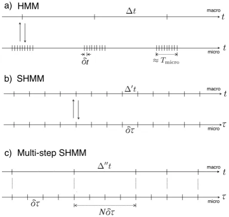
time step is set, ∆t, which is small enough to ad-equately resolve macroscopic variations, but which is much larger than the microscopic time step, δt. For each macroscopic time step there are performed multiple microscopic time steps, such that the time evolved microscopically is roughly equal to the mi-croscopic relaxation time,Tmicro; more than this, and

computational effort is wasted.

A major improvement on this method has recently been proposed by E et al. (2009): the Seamless Het-erogeneous Multiscale Method (SHMM). Here, the micro simulation does not need to be continually re-initialised between macro timesteps, which can be costly: the interaction between the micro and macro solvers is continuous (seamless), as illustrated in Figure 1b. SHMM exploits temporal scale separa-tion in the given problem by running the macro and micro solvers on different clocks (t andτ, respec-tively). The computational time steps, although cou-pled as if they were of equivalent times, are asyn-chronous. The micro model is not reset at every coupling, instead it dynamically adapts to changes in the macro environment (manifested through the constraints applied from the macro solver). Implicit time-averaging of the micro data therefore replaces the explicit time-averaging of most other hybrid methods. This asynchronous coupling has the effect of “fast-forwarding” the macro constraints (from the perspective of the micro-solver); in timescale-separated conditions this produces a good approx-imate response to the macro constraints being ap-plied in real time, provided the SHMM macro time step is sufficiently small. A further advantage of the SHMM approach is that it allows control over how aggressively timescale separation is exploited for computational efficiency (at the expense of er-ror). The ratio between the scales of the micro and macro clocks (which we refer to in this paper as the temporal gearing) directly determines the com-putational saving relative to a simulation that is per-formed entirely using the micro model; in SHMM, the gearing can be set explicitly.

A drawback of SHMM is that in regions of high timescale separation, many more macroscopic time step calculations, and transfers of data, are per-formed than are necessary in HMM; these additional macroscopic computations may not always be neg-ligible in cost. Furthermore, in such conditions, the HMM approach is more accurate, because at indi-vidual macro instants the HMM micro solution is fully relaxed to the actual macroscopic constraint

and not a time-averaged one, as in SHMM.

In this paper we propose a modified time-stepping strategy for exploiting timescale separation: a multi-step SHMM. This approach adopts the same asyn-chronous coupling of two simulation clocks, and the continuous solution of the micro-solver (i.e. no re-initialisation is required), but allows the num-ber of micro time steps per coupling instance, N, to be greater than 1; see Figure 1(c). Figure 2 shows the sequence of solution for each coupling in-stance. The multi-step number,N, provides an ad-ditional control, which can be increased in regions of high timescale separation (where t τ) to ob-tain maximum accuracy and to lower the macro-scopic/coupling overhead, and reduced in regions of low timescale separation (t→ τ) to approach a full microscale simulation. The multi-step approach can thus be viewed as a hybrid of HMM and SHMM, combining desirable features of both: simple con-trol of the computational gearing (saving over a full micro simulation); no requirement for reinitialisa-tion of the micro simulareinitialisa-tion; highest accuracy over the whole range of timescale separation; and fewest macroscopic computations and coupling instances performed in fully scale-separated conditions.

Figure 2: Sequence of solution for the multi-step SHHM, for a single coupling instance. (1) micro data compressed to macro model; (2) macro solver advancement; (3) constraints applied to micro model; (4) micro model advancedNsteps.

2. Time-stepping with timescale separation

In this paper we define a dimensionless timescale-separation number,S, as:

S = Tmacro

T_micro, (1)

whereTmacrois a macroscopic time scale andTmicro

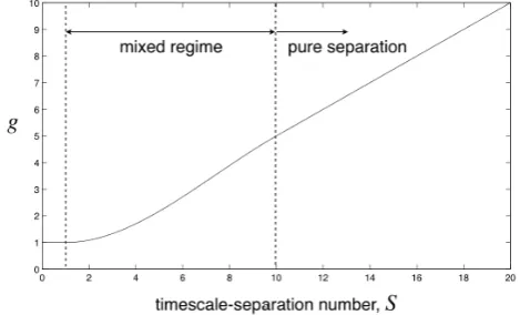
is a characteristic microscopic relaxation period. For S 1, the micro and macro scales are purely sepa-rated; forS =1 there is no separation (i.e. the micro and macro scales act over the same time frame); a “mixed” or transition regime between the two ex-tremes is here defined as 1 < S < 10. The ex-act division between the mixed and pure-separation regimes is arbitrary, in the same way as are the di-visions of rarefaction regimes in terms of Knudsen number (e.g. slip, transition, free-molecular).

Here we define the temporal gearing of a hy-brid approach, g, as the macroscopic time evolved per unit of microscopic time evolved. If the macro solver costs are negligible, this is equivalent to the computational saving compared to a full micro sim-ulation. Clearly, to exploit scale separation fully, at higher timescale-separation numbers the tempo-ral gearing should increase.

The temporal gearing in HMM is the ratio: T_macro/T_micro, i.e., g = S. Depending, though, on the error that is acceptable or the accuracy desired, this particular relationship between temporal gear-ing and timescale separation may not be appropriate. In this respect, the SHMM (and also the proposed multi-step SHMM) has an advantage. Here, the tem-poral gearing is simply the ratio of the two clock time scales,g =t/τ. This means that any functional dependence of the temporal gearing on the timescale separation number can be implemented.

In this paper, we choose a straightforward func-tional relationship between temporal gearing and timescale separation, as follows: when there is no

scale separation, the macro clock should approach the micro clock (i.e. g = 1 at S ≤ 1); when there is pure scale separation (S ≥10), the temporal gear-ing should increase proportionally with the degree of scale separation, (i.e.,g∝S):

g(S)=       

1, forS ≤1,

kS, forS ≥10, (2)

where an increase in the constant of proportional-itykincreases computational saving, at the expense of accuracy. For values ofS in the “mixed” regime (1 < S < 10) we choose the minimum-order poly-nomial that enforces continuity of value and slope of gatS=1 andS=10:

g(S) =a1S3+a2S2+a3S +a4

,for 1<S <10 (3)

where the coefficients an depend on the specific value ofk. Figure 3 shows a plot of temporal gear-inggagainstS, fork=0.25 (note, this is a more con-servative temporal gearing as compared to HMM, which impliesk=1).

Figure 3: Temporal gearing,g, against the timescale-separation number,S;k=0.25.

2.1. Multi-step SHMM

On the other hand, whenS is in the mixed regime, having the micro state converged over a range of pre-vious macro states (as in SHMM), reflects the true micro state more accurately, as it is not locally re-laxed at each macro instant (as in HMM).

The multi-step SHMM we propose seeks to com-bine the best of both approaches over the full range of S. As per SHMM, the micro time step, ∆τ is held constant, and is set by stability/accuracy con-siderations. In SHMM the macro time step can be set directly by the gearing desired (as determined by equations (2)-(3), for example):

∆0

t= ∆τg, (4)

Here, though, differently to SHMM, we allow the number of micro steps per coupling instance,N, to be greater than 1 (as illustrated in Figure 1c). The macro time step is then set according to:

∆00

t= ∆τg N, (5)

under the proviso that it does not exceed the maxi-mum macro time step allowable∆tmax(based on

sta-bility/accuracy considerations).

The most accurate/efficient number of multisteps, N, will depend upon the temporal scale separa-tion, S. Given that for pure timescale separation, a largerNprovides a more accurate solution (as dis-cussed above), we setN to be maximum forS≥10. For non-timescale-separated conditions (S≤1), the macro and micro time steps should be synchronous, (i.e. N=1). For values ofS in the “mixed” regime (1< S < 10), we choose the minimum-order poly-nomial that enforces continuity of value and slope of NatS=1 andS=10:

N(S)=             

1, forS ≤1,

b1S3+b2S2+b3S +b4, for 1<S <10,

Nmax forS ≥10,

(6)

where

Nmax= ∆ t_max

∆τg, (7)

and the coefficientsbnare dependent onNmax.

3. Test cases: transient one-dimensional shear flows

In timescale-separated simulations there are three sources of error: error due to the micro solution; er-ror due to the macro solution; and erer-ror due to the time-step coupling scheme (e.g. SHMM). We re-strict our attention to the latter.

The test cases in this paper are time-dependent flows between parallel plates. Here, the macro model calculates the pressure gradient or the channel-wall velocity, and the micro model calcu-lates the spatial distribution of streamwise velocity (parallel to the walls). For these cases, the macro calculation is trivial, exact and knowna priori. This is convenient, as it allows us to eliminate macro solver error in our evaluation of the alternative time-stepping schemes, and since there is no error in the constraints applied to the micro solver, all error is either from the micro model (which is deliberately kept negligibly small) or error due to the tempo-ral coupling scheme. In all simulations we spec-ify a maximum macro time step∆t_max = T_macro/5, which in practice would be set by macroscopic sta-bility/accuracy requirements.

3.1. Oscillatory Poiseuille Flow

The flow between two parallel plates resulting from an oscillating pressure gradient is a canonical transient case in fluid dynamics. If this is a locally near-thermodynamic equilibrium flow 1 an appro-priate micro model is the one-dimensional Navier-Stokes momentum equation:

∂u ∂t =ν

∂2_u

∂y2 + Π(t), (8)

whereν is the kinematic viscosity, y is a direction perpendicular to the walls, anduis the flow-velocity component parallel to the wall. The micro model is constrained through the time-dependent stream-wise pressure gradient,Π(t). The characteristic mi-croscopic time scale, Tmicro is taken as the startup

time: the time taken, after a suddenly imposed and constantly applied pressure gradient, for the mean velocity to reach 95% of its steady-state value.

The macro model solver, in this example, is the model that calculates the pressure gradient, simply:

Π =_Πˆ _{sin(ωt), (9)}

whereωis the radial frequency of oscillation andt is the macroscopic time. The characteristic macro-scopic time scale is chosen to be the quarter-wave period:

T_macro= π

2ω, (10)

1_{note, timescale separation can be independent, as it is here,}

and thus the timescale separation number at a partic-ular frequency is:

S = Tmacro Tmicro =

π 2ωTmicro

. (11)

We consider a range of oscillation frequencies, span-ning timescale separation numbers fromS=1 to 50. The temporal gearing for a givenS is as described by equations (2) and (3), and as shown in Figure 3 (f=0.25). For the multi-step SHMM the number of micro time steps per coupling instance (N) is calcu-lated using equation (6); Nis plotted in Figure 4 as a function ofS. In evaluating equation (6) and (7), we take∆tmax=Tmacro/5.

Figure 4: Number of micro timesteps per coupling instance,N, against the timescale separation number,S.

For evaluating the accuracy of SHMM and the multi-step SHMM, a classical analytical solution to the full problem (equations 8 and 9) is used:

u(y)=< (

eiωt Πˆ

ω A1(y, η) )

, (12)

where

A1(y, η)= 1−

coshη

(y−h/2)(i+1) coshηh

(i+1)/2 !

, (13)

andη=√(ω/2ν), withhthe channel height.

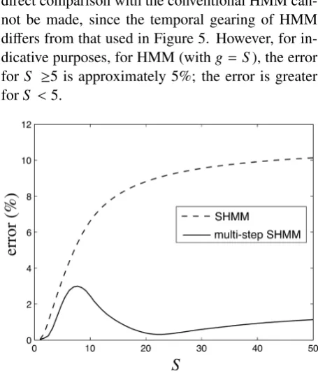
Figure 5 compares the accuracy of the SHMM and the multi-step SHMM. For all values of S considered, the multi-step method is more accu-rate (for the same gearing); for S 1 the multi-step approach is over 8× more accurate. Further-more, the multi-step HMM involves approximately 1600×fewer macroscopic calculations and instances of coupling (though, in this illustrative example, the macroscopic calculation has negligible cost). Note,

direct comparison with the conventional HMM can-not be made, since the temporal gearing of HMM differs from that used in Figure 5. However, for in-dicative purposes, for HMM (withg= S), the error forS ≥5 is approximately 5%; the error is greater forS <5.

Figure 5: Maximum error (%) (over time) of mean velocity (overy) againstS. S-HMM (dashed line) against multi-step S-HMM (solid line).

3.2. Oscillatory Couette Flow

Another canonical transient flow in fluid dynam-ics is that between two plates generated by the oscil-latory transverse motion of one wall relative to the other. In this case, the macro model provides the constraint on the micro solution in the form of an imposed wall velocity, i.e.:

u(0)=Uˆwallsin(ωt), (14)

where ˆUwallis the amplitude of the moving wall (at y=0). For evaluating the accuracy of SHMM and the multi-step SHMM, a classical analytical solution to the full problem (equations 8 and 14) is used:

u(y)==neiωt Uˆwall A2(y, ξ) o

, (15)

where

A₂(y, ξ)=

cosh (ξy)−coth(ξh) cosh(ξy), (16)

Figure 6: Maximum error (%) (over time) of mean velocity (overy) againstS. S-HMM (dashed line) against multi-step S-HMM (solid line).

3.3. Non-equilibrium Oscillatory Poiseuille Flow

At atmospheric pressures, gas flow through micro/nano-channels can be highly non-equilibrial (Reese et al. (2003)). The final example consid-ered here, is isothermal oscillatory Poiseuille flow (as in §3.1) of a monatomic gas in rarefied/ non-equilibrium conditions.

The degree of departure from local thermody-namic equilibrium in a gas (the state of rarefaction), is expressed by the Knudsen number:

Kn= λ

h, (17)

where λ is the mean distance between molecular collisions, and h is the characteristic macroscopic length scale; here, this is the channel height.

The micro model chosen here is the BGK Boltz-mann equation:

∂f ∂t +vˆ

∂f ∂y +

∂f

∂uˆFx(t)=−

(f − feq)

ξ (18)

where f is the molecular distribution function, feqis the equilibrium distribution,ξis the molecular relax-ation time, Fx(t) is the time-dependent body force (equivalent to an oscillatory pressure gradient) and

ˆ

u, ˆvare the x−andy-components of molecular ve-locity, respectively. The molecular relaxation time for the BGK model is given byξ = µ/p, whereµis the dynamic viscosity and pis the gas pressure.

We obtained solutions for the micro model (18) using a discrete velocity method (DVM) similar to that used by Valougeorgis (1988). This numerical

scheme, which uses Gaussian quadrature to integrate in velocity space, has been tested extensively against a host of problems in rarefied gas dynamics and has proved to be both accurate and highly efficient (see, e.g., Naris and Valougeorgis (2005); Valougeorgis (1988); Valougeorgis and Naris (2003)).

As in previous sections, the macro model solver for the oscillatory driver is trivial. Simply:

Fx(t)=Fxˆ sin(ωt). (19)

All parameters relating to the SHMM and multi-step SHMM are identical to those in§3.1.

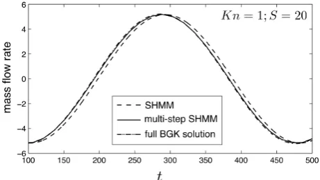
Figure 7 shows the time evolution of mass flow rate resulting from the oscillatory forcing (19) over a selected period of the cycle; for this simulation Kn = 1 and the timescale separation S=20. The mass flow rate is normalised with the Navier-Stokes prediction of mass-flow-rate amplitude (notice that the mass-flow-rate amplitude predicted by the full BGK solution is over five times that of the Navier-Stokes equations). The SHMM is compared to the multi-step SHMM; both solutions produce a good prediction with a temporal gearing of five (in this case, effectively a factor of five computational sav-ing over the full BGK solution). However, the multi-step SHMM is still significantly closer to the full BGK solution, both in terms of amplitude and phase. As was the case in section§3.1, the multistep SHMM obtains this better prediction, with far fewer macroscopic calculations and coupling instances. In this case, whereS 1, an equivalent HMM solu-tion would be as accurate as the multi-step SHMM (for a gearing ofg=S).

Figure 7: Time evolution of mass flow rate (normalized with the Navier-Stokes prediction of mass-flow-rate amplitude) forKn=

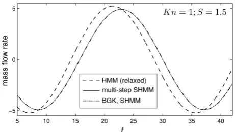
Figure 8: Time evolution of mass flow rate (normalized with the Navier-Stokes prediction of mass-flow-rate amplitude) for

Kn=1 and a timescale separation number,S=1.5; fully relaxed HMM solution (dashed line); multi-step SHMM (solid line); full BGK solution and SHMM (dashed and dotted line)

Figure 8 shows the time evolution of mass flow rate resulting from a higher frequency forcing; for this simulation Kn = 1 and the timescale separa-tionS=1.5. In this case, both the SHMM and multi-scale SHMM are barely distinguishable from the full BGK solution. This is to be expected, as the tempo-ral gearing in this case isg≈1. A HMM solution is also plotted to demonstrate that, clearly, fully relax-ing the micro solution to the macroscopic constraints is inaccurate at low degrees of scale separation.

4. Summary and Conclusions

A multi-step version of the seamless heteroge-nous multiscale method (E et al. (2009)) has been proposed. It shares the main advantages of SHMM over HMM, e.g.:

1. the micro-solver does not require re-initialisation at every macro time step;

2. the temporal gearing can be controlled in a straightforward manner by adjusting the ratio of the micro and macro clocks;

3. it can be used in both timescale-separated and non-timescale-separated conditions, thus ap-propriate for an adaptive scheme with time-varying scale separation;

while retaining the accuracy and macroscopic effi -ciency of HMM:

1. when timescales are purely separated, multi-step SHMM provides a more accurate result; 2. and in such conditions, far fewer coupling

in-stances and macroscopic calculations are re-quired.

The multi-step scheme can thus be viewed as an amalgam of HMM and SHMM: a combination of the best features of both methods.

We have presented results from three transient shear flow problems. In each case, the macro model computation is trivial (i.e. the evaluation of a sine function). This has allowed us to focus on error arising from the particular time-stepping scheme. Two micro models have been considered: a Navier-Stokes micro model and a Boltzmann BGK micro model. In each of the three examples, the multi-step SHMM demonstrated significantly greater accuracy than the SHMM, and at a fraction of the number of coupling instances and macroscopic computations.

Acknowledgments This research is financially supported by the EPSRC Programme Grant EP/I011927/1. The authors would like to thank Prof. Dimitris Valougeorgis for providing a well-documented DVM code that helped to generate the BGK results presented in this paper.

References

E, W., Engquist, B., Li, X.T., Ren, W.Q., Vanden-Eijnden, E., 2007. Heterogeneous multiscale methods: A review. Com-munications in Computational Physics 2, 367–450. E, W., Ren, W.Q., Vanden-Eijnden, E., 2009. A general

strat-egy for designing seamless multiscale methods. Journal of Computational Physics 228, 5437–5453.

Naris, S., Valougeorgis, D., 2005. The driven cavity flow over the whole range of the knudsen number. Physics of Fluids 17.

Reese, J.M., Gallis, M.A., Lockerby, D.A., 2003. New direc-tions in fluid dynamics: non-equilibrium aerodynamic and microsystem flows. Philosophical Transactions of the Royal Society a-Mathematical Physical and Engineering Sciences 361, 2967–2988.

Valougeorgis, D., 1988. Couette-flow of a binary gas-mixture. Physics of Fluids 31, 521–524.