IAC-12-C1.4.6
EXTENSION OF FINITE PERTURBATIVE ELEMENTS FOR MULTI-REVOLUTION, LOW-THRUST PROPULSION TRANSFER OPTIMISATION
Federico Zuiani
Ph.D. Candidate, School of Engineering, University of Glasgow, United Kingdom, [email protected]
Massimiliano Vasile
Reader, Department of Mechanical and Aerospace Engineering, University of Strathclyde, United Kingdom, [email protected]
This paper presents an extension of the analytical solution for perturbed Keplerian motion of a spacecraft under the effect of a low-thrust action (Zuiani et al., Acta Astronautica, 2011). The new formulation will include the possibility for treating two different thrusting modes, i.e. with a fixed thrust direction either in a rotating or in an inertial frame. Moreover the contribution of the J2 effect is also included in the analytical formulae. It will be shown
that this approach allows for the fast computation of long, many revolution spirals while maintaining adequate accuracy, and it is able to include the combined actions of different perturbations.
The proposed approach will also be applied to the case of a spacecraft with a low-thrust engine, which is injected into a Geostationary Transfer Orbit and will subsequently use its on-board propulsion to transfer to a final circular orbit around the Earth. The completion of the whole transfer might require several spirals and this makes the use of a full numerical propagation prohibitive on a sequential machine. In the proposed method, the thrusting pattern, duration and start of each thrusting arc, is defined through a parameterised function. The spiral is then propagated with the above-mentioned analytical approximation. A direct optimisation approach is then used to optimise these control parameters in order to minimise the propellant cost of the transfer, given a fixed transfer time and a set of boundary conditions.
I. INTRODUCTION
The design of low-thrust (LT) trajectories requires the definition of the thrust profile that satisfies a two-point boundary value problem. The scope of this work is to provide a computationally efficient way to determine a good approximated solution to this problem with a representation of the control profile comparable to more accurate but computationally expensive approaches.
In the literature, the problem has been tackled in a number of different ways1,2, generally classified in two
families: indirect methods and direct methods. Indirect
methods3,4,5 translate the design of a low-thrust
trajectory into the solution of an optimal control problem and derive explicitly the associated first-order optimality conditions. The first-order optimality conditions are a system of mixed differential-algebraic equations (DAE). Shooting, multiple-shooting, collocation and approximated analytical approaches have been proposed to solve the DAE system and satisfy the boundary conditions.
Direct methods6,7, instead, do not derive the
optimality conditions but transcribe the differential dynamic equations of motion into a system of algebraic equations and then solve a nonlinear programming problem. Numerical integration and collocation techniques have been proposed to transcribe the differential dynamic equations.
A number of direct methods8,9,10 have been
successfully applied to interplanetary transfer design. However, most of them are ill-suited for LT many-revolution transfers, like all typical orbit change manoeuvres around the Earth. Given the particular thrusting pattern and duration of this type of transfer, the associated number of control parameters can easily render them intractable or, for the purposes of a preliminary estimation, at least computationally very expensive.
In past works, other authors have already proposed approaches to the design of low thrust, many-revolution transfers, based on analytical solutions to an optimal orbit raising problem under the assumption of small eccentricity11,12,13 or through averaging techniques14,15.
However, few proposals16,17 exist for treating generic
many-revolution transfer problems. Adding to this, they sometime require numerical integration of the perturbed motion and might therefore be expensive to evaluate.
Recently, Bombardelli et al.18, proposed an
analytical solution for the case of purely tangential thrust which promises a fast and accurate propagation constant thrust profiles over extended periods of time.
Zuiani et al.19 presented a closed form analytical
same analytical formulation has been used in a previous work20 to propagate the motion of an asteroid under the
effect of an ablation-induced thrust. In another work21, it
has been applied to the design of Low-Thrust, many revolution transfers.
In this paper, an extension of the analytical formulation is presented which now includes also the contribution of a constant inertial thrust and the J2
effect. Adding to this, the approach to the solution of the time equation has been revised and improved compared to the previous work. It will be shown that the resulting analytical approximate solution is suitable for the fast and accurate propagation of long spiralling trajectories in which different perturbative actions are present. Moreover, if combined with averaging techniques, further gains in terms of computational time are possible. Finally, the analytical propagator will be combined with a simplified parameterisation for the thrusting pattern to provide a fast and flexible tool for the design of spiralling transfer, like for example a simple Geostationary Transfer Orbit (GTO) to Geostationary Earth Orbit (GEO) circularisation.
II. PROBLEM DEFINITION
II.I Equations of Motion
Let the state of the spacecraft be expressed in terms of non-singular Equinoctial Elements22:
1
2
1
2
sin
cos
tan sin
2
tan cos
2
a
P
e
P
e
i
Q
i
Q
L
X
[1]then, the perturbed Keplerian motion is governed by Gauss’ planetary equations:
3
2 1
1
1
1 2
2 2
2
1 2
1
2 2 1
1 2
sin
cos
2
sin
cos
cos
sin
cos
sin
sin
cos
cos
sin
sin
1
2
r
r
h
r
h
h
da
a
P
L P
L a
a
dt
B
dP
a
B
L a
dt
P
L a
Q
L Q
L
P
a
dP
a
B
L a
dt
P
L a
Q
L Q
L
P
a
dQ
B a
L
Q
Q
L
L
L
L
L
L
L
a
L
dt
dQ
2 2
21 2
cos
1
2
hB a
L
Q
Q
a
dt
L
[2]
with:
2 2 2
1 2
1 2
1
1
1
sin
cos
B
P
P
e
L
P
L P
L
[3]where ar, aθ, ah, are the components of the thrust
acceleration in the radial-transverse-normal (r-θ-h) reference frame, which can also be expressed in terms of modulus-azimuth-elevation as:
cos cos
cos sin
sin
rh
a
a
a
[4]
As shown in19, if one assumes that the modulus of
the thrust acceleration is small compared to the local gravitational acceleration, one can write:
2 3 3
2
dt
r
a
B
dL
h
L
[5]
3 2 2 1 2 4 2 1 2 1 3 2 1 2 2 3 4 2 2 2 2 3 2 1 2 1 sin co sin cos 2 1 cos sin cos sin sin cosc s i
s
o s n
r
r
h
r
P L P L
da B a a
dL L L
dP B L
a
dL L
P L
a
L L
Q L Q L
P a
L
dP B L a
dL L P L a L a a L a L L
Q L Q L
P
3 4 2 2 2 11 2 3
4 2
2 2
2
1 2 3
2 sin 1 cos 1 2 h h h a L
dQ B Q Q L
dL L
dQ B L
Q Q a
dL L a a a [6]
Or, in vector form:
, , , , ,
r h
d
F
L
a a a
dL
E
E
[7]By integrating [7] in L, keeping the remaining equinoctial elements as constants, one can write a first-order expansion of E with respect to L as:
0 0 0 0 1 , , , , L LL L
F L L
dL
E E E
E E
[8]
As it will be shown in the next sections, the integral term in [8] can be expressed analytically for some special acceleration patterns.
The time equation can be similarly expressed as:
00 1
( )
t L
t
t
[9]Note that the zero-order term t00 is not just the time
corresponding to L0, but includes also the time variation
given by unperturbed Keplerian motion, which is omitted here but can be easily derived. The first-order term t1 can be derived from [5] and integrated in L:
1 0 1 L L
d
dt
t
dL
d
dL
[10]Considering that: 1 1 2 2 dP
d dt da d dt d dt
d dL d da dL d dP dL dP d dt
d dP dL
[11]and, from [8]:
1
11 2
1 21
dP
dP
da
a
P
P
d
d
d
[12]after some manipulations, one can write:
0 2 1 1 2 2 1 11 2 3 2 21 2 3 2 3 2 3 sin 2 3 cos 2 L L a a B t B P La B P
P L
B L
L L
L L P
[13]Note that the presence of the terms a1, P11, P21
essentially implies a double integration between L0 and
L.
II.II Constant Trust in the r-θ-h frame
If one assumes a constant thrust modulus and
direction in the r-θ-h frame, then the system of
equations in [8] can be integrated analytically, leading to:
3 2 0 00 20 2 10 2 11
4 2 0 0
1 10 2
13 10 3 2 20 10 3 20 3
4 2 0 0
2 20 2
13 20 3 2 10 10 3 20 3
4 2
2 2 0 0
1 10 1 2 3
4 2 2 0 0
2 20 1
2
2
2
1
1
s c r
c r s s
c s h
s r c c
c s h
s h
B
a a
P I
P I
a
I a
B
P
I a
I P
I
a
P Q
Q
a
B
P
P
a
I P
I
a
P Q
Q
a
B
Q
Q
a
a
P
I
I
I
a
I
I
I
I
a
a
Q
Q I
B a
Q
Q
Q
2
2 c3 h
Q I a
[14]
where the terms expressed as Ixx are integrals in L in
0 0 0 0 0 1 0cos
sin
1
L L L L L Lcn n sn n
n n
L
L
I
dL I
dL
L
L
I
dL
L
[15]where Φ0 is the term in [3] evaluated with P10 and
P20. The analytical form for these integrals is omitted
here for the sake of conciseness.
Regarding the first-order term of the time equation [13], as already noted in the previous section, some of the integrals in [15] are multiplied by a function of L and again integrated between L0 and L. For the term
depending from a1, it has been possible to find an
analytical expression, leading to:
7 0
1
3
3 0cos
c
os
I
t1sin
t2a
I
t
B
[16]where:
0 12 1 13 0 0 2 11 t L L tI
I
L
I
L d
I
L
I
[17]II.III Constant inertial thrust
A constant acceleration in the inertial reference frame can be expressed, in the r-θ-h frame, as a function of the longitude L:
0 0cos
sin
cos
sin
cos
In In r h Ina
L
a
a
L
[18]where γ0 derives from the acceleration azimuth α0 at
L0, i.e.:
0 0
L
0
[19]Substituting [18] into [6], and after some manipulations, one can obtain an expression analogous to [14]:
0 3 2 0 010 12 2 0 20 12 2 0
1 10 4 2
0 0
10 3 12 2 3 0 10 3 1 1 3 0
20 10 3 20 3 2 20 4 2
0 0
20 3 1 1 3 0 20 3 12 2 3
2
cos
cos
sin
cos
cos
sin
cos
cos
s
sin
s c s sc c s
c s
s c s
c c
a a
B
P I
I
P I
I
P
B
P I
I
P
a
P
a
I
I
I
P
P P
B
P I
I
P
I
I
Q
Q I
a
I
I
0 10 10 3 20 3 4 22 2 0 0
1 10 1 2 3
4 2
2 2 0 0
2 20 1 2 3
in
1
sin
sin
2
sin
2
1
c s s cP
B
Q Q
Q
Q
I
B
Q
Q
Q
I
I
a
Q
Q I
Q
a
[20]where the integral terms are given by:
0 0
cos
sin
L j k
jcksn n
L
L
L
I
dL
[21]Similarly, the first-order perturbative term in the time equation translates into:
7 5 0 01 13 10 3
3 20
10 0
12 0 0
0
0 3 12
0 0 3 cos 1 sin co s n s sin i s s a
t B I P I
P P L I L L I I L
[22]II.III J2 perturbation
The components of the J2 perturbation in the r-θ-h
2 2 2 2 2 2 1 28 4 2
4
2 2 8 2 4
4 1 2 2 2 2 1 1 2 1 2
8 2 4
2 2 4
3 12 cos sin
2
1
12 cos sin
cos sin cos sin 1 6 J h r J J R
a Q L Q L
B a G
L R
a Q L Q L
J
J
J B G a
Q L Q L L
R
a Q L Q L
B G a
Q Q L
[23]
where J2 is the well-known spherical Harmonic
coefficient, R is the planetary radius and G is:
2 2
1 2
1
G
Q
Q
[24]Substituting [23] into [6] and with the procedure previously described one can write the first-order
variation of the Equinoctial Elements due to the J2
perturbation. In a compact form, this can be expressed as:
1 1 2 2 2 20 6 2 ,
0
0 0
2 2
1 10 2 2 ,
0
0 0 0
2 2
2 20 2 2 ,
0 5 3 1 1 5 5 4 1 1 5 5 4 0 1 1 0 0 1 3 cos sin cos sin 3 cos sin cos sin 3 cos sin cos sin a i j P i j i j i j i j i j i j P i j L i j i j L P i j i j P J R
a a C L L
B G a
L L
J R
P P C L L
B G a
L L C L L
J R
P P C L L
B G a
L L C L L
Q
1 1 2 2 2 210 2 ,
0
0 0 0
2 2
2 20 2 ,
0 3 3 4 1 1 3 3 4 1
0 0 0
1 3 cos sin cos sin 3 cos sin cos sin Q i j Q i j i j i j Q i j L i j i j Q i j L J R
Q C L L
B Ga
L L C L L
J R
Q Q C L L
B Ga
L L C L L
[25]where the coefficients Ci,j and CL are polynomial
functions of P10, P20, Q10, Q20. Note that there is no
linear component in L in the expansion of a, confirming the known result that J2 is not inducing any net variation
of the semi-major axis and thus the energy. There is, on the other hand, a short-term periodic variation of a over one orbital revolution. The remaining equinoctial elements, present both a short-term periodic variation and a secular one, which is linear with respect to L.
III. NUMERICAL ANALYSIS
III.I Accuracy
In order to determine the accuracy of the analytical first-order expansions described in the previous section, a simple test case will be proposed. For each of the three expansion formulae, an initial orbit around the Earth will be propagated analytically with a perturbative acceleration and for an arbitrary number of orbits. The propagated states will be then compared with the results of a full numerical integration of Gauss’ variational equations. Both propagations are performed with MatLab and the numerical integration is performed with ode113, implementing an Adams-Bashfort predictor-corrector method.
In the first case, an initial orbit around the Earth is considered, with the orbital parameters as in Table I.
a e i Ω ω θ
[image:5.595.84.291.326.578.2]7000 km 0.1 6° 0° 10° 0°
Table I: Initial orbit parameters
The perturbative acceleration in the r-θ-h frame is 10-4 m/s2, with α=π/2 and β=π/6. The orbital motion is
[image:5.595.311.521.388.559.2]propagated for 20 orbits.
Fig. I: Constant r-θ-h acceleration: Semi-major axis.
Fig. I shows the behaviour of semi-major axis for the analytical and numerical propagation. One can see that the error is quite negligible even after 20 orbits and in effect it reaches only 0.1 km, as shown in Fig. II.
0 20 40 60 80 100 120 140
Fig. II: Constant r-θ-h acceleration: error on semi-major axis.
Fig. III and Fig. IV similarly show the behaviour of P1 and Q1 and reveal a very good matching of the
first-order expansion with the ode113-integrated time
behaviour. P2 and Q2 show similar behaviours.
[image:6.595.310.522.108.285.2]Fig. III: Constant r-θ-h acceleration: P1.
Fig. IV: Constant r-θ-h acceleration: Q1.
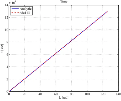
Fig. V: Constant r-θ-h acceleration: Time.
Fig. V shows the time as computed from [13] and from the exact integration of the time equation. On can note that the correction term from a1 is already adequate
to accurately compute the time flown and the error compared to the numerical integration, as shown in Fig. VI, is indeed very low, less than 5 sec after 20 orbits. Moreover, along the first orbit it is by all means negligible. This approximation lowers the error by at least one order of magnitude over the previous
formulation, found in19, which neglected the second
integration over L. Note also that a good computation of the time is essential, in particular when one has to use
this datum to compute the ΔV corresponding to the
propagated thrusting arc. It also very important to note that the analytical propagation has a considerable edge in terms of computational time because it required 10-3
sec compared to 0.9 sec of ode113, corresponding to
[image:6.595.70.286.358.724.2]almost 1000 times speed up.
Fig. VI: Constant r-θ-h acceleration: error on time.
In the second case, the same initial orbit is
propagated, this time with a 10-4 m/s2 constant
0 20 40 60 80 100 120 140
0 0.02 0.04 0.06 0.08 0.1 0.12
Error on semi−major axis
L [rad]
Δ
a [km]
0 20 40 60 80 100 120 140
0.0173 0.0173 0.0173 0.0173 0.0174 0.0174 0.0174 0.0174 0.0174 0.0174 0.0174
Parameter P1
L [rad] P1
Analytic ode113
0 20 40 60 80 100 120 140
−12 −10 −8 −6 −4 −2 0 2 4 6
8x 10
−6 Parameter Q1
L [rad] Q1
Analytic ode113
0 20 40 60 80 100 120 140
0 2 4 6 8 10 12 14x 10
4 Time
L [rad]
t [sec]
Analytic ode113
0 20 40 60 80 100 120 140
0 1 2 3 4 5 6
Error on time
L [rad]
Δ
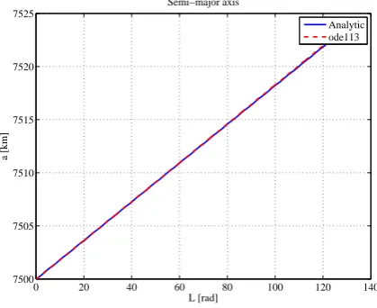
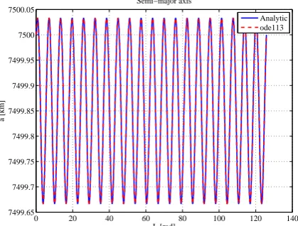
[image:6.595.313.520.508.680.2]acceleration in the inertial reference frame. Fig. VII shows that the analytic approximation easily matches the periodic behaviour of the semi-major axis.
[image:7.595.74.285.332.495.2]Fig. VII: Constant inertial acceleration: Semi-major axis.
[image:7.595.308.521.332.695.2]Fig. VIII: Constant inertial acceleration: P1.
Fig. IX: Constant inertial acceleration: Q1.
Similarly, Fig. VIII and Fig. IX show that the approximated values for P1 and Q1 match quite closely
the numerical ones. Q1 shows a more apparent deviation
but nevertheless the error is still in the range of 10-6.
Analogous considerations apply to P2, Q2 and t, the
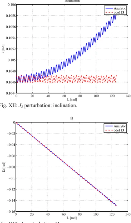
graphs of which are not reported for c1onciseness. In the third case, the initial orbit is propagated under J2 perturbation only. As in the previous two cases, the
behaviour of the Equinoctial elements shows a good matching with the results of numerical integration. However, a critical point is represented by parameters Q1 and Q2. From Fig. X and Fig. XI one can see that the
matching on Q1 is good and at the same time the error
on Q2 is not considerable. If these values are converted
to inclination and right ascension of the ascending node Ω, one can see that the accuracy for the latter is still very good, but for the former there is a long term
deviation. This negates the known result that J2
perturbation has no secular variation of inclination. While this deviation is almost negligible along a single orbit, it might be problematic when a long time horizon is considered, and should be taken into account.
Fig. X: J2 perturbation: Q1.
Fig. XI: J2 perturbation: Q2.
0 20 40 60 80 100 120 140
7499.65 7499.7 7499.75 7499.8 7499.85 7499.9 7499.95 7500 7500.05
Semi−major axis
L [rad]
a [km]
Analytic ode113
0 20 40 60 80 100 120 140
0.0156 0.0158 0.016 0.0162 0.0164 0.0166 0.0168 0.017 0.0172 0.0174 0.0176
Parameter P 1
L [rad] P1
Analytic ode113
0 20 40 60 80 100 120 140
−12 −10 −8 −6 −4 −2 0 2 4 6
8x 10
−6 Parameter Q1
L [rad] Q1
Analytic ode113
0 20 40 60 80 100 120 140
−8 −7 −6 −5 −4 −3 −2 −1
0x 10
−3 Parameter Q1
L [rad] Q1
Analytic ode113
0 20 40 60 80 100 120 140
0.0517 0.0518 0.0519 0.052 0.0521 0.0522 0.0523 0.0524 0.0525 0.0526
Parameter Q2
L [rad] Q2
[image:7.595.72.285.518.703.2]Fig. XII: J2 perturbation: inclination.
Fig. XIII: J2 perturbation: Ω.
Given the limited entity of element variations with the perturbation considered it is also possible to combine the three first-order expansion seen before into a single approximate solution for Keplerian motion perturbed by constant r-θ-h and inertial acceleration plus J2 perturbation. This involves in a simple application of
the Superposition Principle and consists in simply adding up together the first-order terms which appear in equations [14], [20] and [25]. Fig. XIV to Fig. XVII show the error of propagation performed with the same perturbations as in the previous three cases combined together. The mismatch with numerical integration is not considerably worse than the cases in which the perturbations are considered separately, confirming the possibility of a linear superposition of the perturbative effects.
Fig. XIV: Combined perturbations: error on semi-major axis.
[image:8.595.311.522.305.472.2]Fig. XV: Combined perturbations: error on P1.
Fig. XVI: Combined perturbations: error on Q1.
0 20 40 60 80 100 120 140
0.1044 0.1046 0.1048 0.105 0.1052 0.1054 0.1056 0.1058 0.106
Inclination
L [rad]
i [rad]
Analytic ode113
0 20 40 60 80 100 120 140
−0.16 −0.14 −0.12 −0.1 −0.08 −0.06 −0.04 −0.02 0
Ω
L [rad]
Ω
[rad]
Analytic ode113
0 20 40 60 80 100 120 140
0 0.05 0.1 0.15 0.2 0.25 0.3 0.35
Error on semi−major axis
L [rad]
Δ
a [km]
0 20 40 60 80 100 120 140
0 0.5 1 1.5 2 2.5 3
3.5x 10
−4 Error on P1
L [rad]
Δ
P1
0 20 40 60 80 100 120 140
0 1 2 3 4 5 6x 10
−5 Error on Q1
L [rad]
Δ
[image:8.595.313.521.502.675.2]Fig. XVII: Combined perturbations: error on time.
II.II Accuracy over a single revolution
It is also interesting to analyse the behaviour of the error for a propagation of a complete orbital revolution. The main idea is that of using the analytical formulae to propagate long multi-revolution transfers by computing the first-order variation of Equinoctial Elements over a single orbit and then updating each time the reference initial conditions E0 for the following orbit. In this
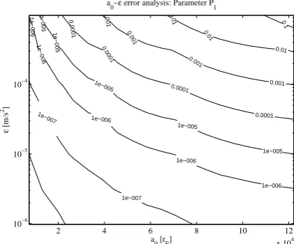
sense, the aim of this analysis is to estimate the error accumulated over one orbit as a function of the magnitude of the perturbative acceleration ε and of the semi-major axis a0 of the initial orbit. The latter, in
particular, is important because it determines the size of the orbit and thus the magnitude of the gravitational acceleration and at the same time the orbital period, i.e. the time length of the propagation. Therefore, a number of initial Earth-centred orbits with eccentricity 0.1 and variable a0 are propagated with different ε, constant in
the r-θ-h frame, with α=π/2 and β=0. Fig. XVIII shows the maximum error on the semi-major axis as a function of a0 and ε. As is intuitively known, one can see that the
error increases with these two parameters. In particular, for large semi-major axis values and ε=10-3 m/s2 the
deviation easily attains more than 104 km, clearly not
acceptable under any circumstances. However one should consider that 10-3 m/s2 is a performance level
hardly attainable with the current electric propulsion technology. If the acceleration is instead in the typical range of 10-4-10-6 m/s2 the resulting propagation error is
acceptable even for relatively large orbits. Note also that all orbits in the LEO to GEO class are integrated very accurately, with errors which are of a few kilometres at worst. Moreover if the error is evaluated in relative terms even an error of 101 km can be acceptable for an
initial orbit of 105 km in the case of a fast preliminary
[image:9.595.311.522.445.620.2]analysis.
Fig. XVIII: Maximum error on a over a revolution w.r.t. a0
and ε.
A similar behaviour is also found in Fig. XIX for P1
and in Fig. XX for the time t. The former is closely related to the orbit eccentricity and therefore it is desirable to keep the error per orbit below 10-5-10-6
which, as shown in the graph, can be attained in most
cases except for high a0, large ε combinations.
Analogous considerations apply to the error on time, in the sense that an error of 103 sec is not acceptable for a
LEO or GEO but might still be tolerated for a very large orbit of 105 km of semi-major axis, which means that its
orbital period is 3.14·105 sec.
Fig. XIX: Maximum error on P1 over a revolution w.r.t. a0 and
ε.
0 20 40 60 80 100 120 140
0 5 10 15 20 25 30
Error on time
L [rad]
Δ
t [sec]
0.0001
0.001 0.001
0.01
0.01
0.01
0.1
0.1
0.1
0.1
0.1
1
1
1
1
1
1
0
10
10
10
10
100
100
100
100
1000
1000
1000 10000
10000
a0 [rE]
ε
[m/s
2]
a
0−ε error analysis: Semi−major axis [km]
2 4 6 8 10 12
x 104
10−6
10−5
10−4
1e−007
1e−007
1e−006
1e−006
1e−006
1e−006
1e−006
1e−005
1e−005
1e−005
1e−005
1e−005
0.0001
0.0001
0.0001
0.0001
0.001
0.001
0.001
0.001
0.01
0.01
0.01
0.1
a
0 [rE]
ε
[m/s
2]
a
0−ε error analysis: Parameter P1
2 4 6 8 10 12
x 104
10−6
10−5
Fig. XX: Maximum error on t over a revolution w.r.t. a0 and ε.
III. TEST CASES
III.I GTO Orbit escape propagation
In this first test case, the aim is to assess the suitability of the proposed analytical approach for the long term propagation of a long, spiralling trajectory. Starting from an initial GTO orbit, with parameters as in Table II, an acceleration of 10-4 m/s2 is applied along the
θ direction until escape conditions are reached (i.e. e=1).
a e i Ω ω θ
[image:10.595.310.521.142.313.2]24478 km 0.73 6° 0° 10° 0°
Table II: GTO orbital parameters.
In order to contain the increase of the propagation error, the reference conditions (as for example in [8]) are updated twice per orbit. This means that the analytical formulae are also evaluated twice per orbit. Note also that, the pure transverse control profile is sub-optimal but nevertheless provides a good approximation of an optimal escape spiralling trajectory. The same acceleration is integrated numerically with ode113 until escape conditions are reached.
Fig. XXI and Fig. XXII show the variation of the semi-major axis and eccentricity and reveal the typical pattern of an escape trajectory from a very elliptical
orbit15 where first, one has a reduction of the
eccentricity to almost zero, followed by a sudden increase up to one during the last few orbits. Simultaneously, there is also a steep increase in the semi-major axis. The fitting between the analytical and numerically propagated spirals is very good up until the last few orbits when the escape conditions are approached. This is due to the fact that, for semi-major
axis above 105, the element variation along a single
orbit is considerable and the first-order perturbative expansion starts losing its validity. A simple mitigation
[image:10.595.310.520.341.519.2]action might be for example that of increasing the reference condition update frequency above a certain threshold on the semi-major axis.
[image:10.595.307.523.364.698.2]Fig. XXI: GTO escape: semi-major axis.
Fig. XXII: GTO escape: eccentricity.
Fig. XXIII: GTO escape: relative error on radius.
1
10
10
10
10
0
100
100
100
100
10 00
1000
1000
1000
10000
10000
a0 [rE]
ε
[m/s
2]
a
0−ε error analysis: Time [sec]
2 4 6 8 10 12
x 104
10−6
10−5
10−4
0 50 100 150 200 250 300 350
104
105
106
107
108
Semi−major axis
Orbits
a [km]
Analytic ode113
0 50 100 150 200 250 300 350
0 0.1 0.2 0.3 0.4 0.5 0.6 0.7 0.8 0.9 1
Eccentricity
Orbits
e
Analytic ode113
0 50 100 150 200 250 300 350
10−7
10−6
10−5
10−4
10−3
10−2
10−1
100
Error on radius
Orbits
[image:10.595.66.291.432.465.2] [image:10.595.311.521.531.704.2]Fig. XXIII shows that in relative terms, the error in terms of radius also remains very low up until the 300th
orbit when it quickly climbs much over 1%.
III.II Orbit raising with Solar Radiation Pressure In the second test case, the long term propagation of an initial GEO under the combined effect of a thrust acceleration along the θ direction and solar radiation pressure (SRP) perturbation. Initial spacecraft mass is 1000 kg, engine thrust is 10-2 N and specific impulse is
3000 s. The cross sectional area used to compute SRP acceleration is 1200 m2, a value which will give a
non-negligible perturbative acceleration. At departure, the Sun lies at the Summer Solstice point. Propagation time is set at two years. This time, propagation is performed through averaging of the orbital elements variation computed analytically along an orbit. The SRP direction is considered to be constant along an orbit, therefore allowing the use of the formulas in Eq. [20]. However, the secular variation of the Sun-Earth direction is still accounted for in the integration of the averaged quantities. The averaged propagation is performed with
MatLab®’s ode23 which implements a Runge-Kutta
integration method. Again, the results are compared to a
full numerical integration with ode113. CPU time
[image:11.595.310.522.345.519.2]required by the averaged analytic propagation was 0.077 s while the full numerical integration required 3.76 s. Fig. XXIV shows the monotonic increase of the semi-major axis due to engine thrust, revealing also the good match between the two propagation techniques.
Fig. XXIV: GEO raising with SRP: semi-major axis.
Fig. XXV shows the long term variation of orbital eccentricity, with a period of one year, due to the SRP effect. The curve of the numerical integration appears to be wider because the short term variations along a single orbit are computed and plotted too, which is not the case for the averaged one. SRP also produces a small long term deviation of the inclination due to the
relative angle between the Ecliptic plane and the Equatorial plane, in which lies the initial GEO.
Fig. XXV: GEO raising with SRP: eccentricity.
Fig. XXVI: GEO raising with SRP: inclination.
III.III GTO-GEO Orbit circularisation
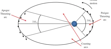
In the third test case, an initial GTO orbit is circularised into a Geostationary Orbit in a specified transfer time. In order to do this, a parameterisation similar to the one presented in21 is used to lower the
number of optimisation parameters in LT, multi-revolution transfers. This envisions dividing each orbit into 4 sectors, as shown in Fig. XXVII: a Perigee thrusting arc, an Apogee transfer arc and two coasting arc in between. The first, of amplitude ΔLp, is meant
ideally to alter apocenter altitude by thrusting in either way along the θ direction. Similarly, the second alters the pericenter altitude by thrusting along θ around the apoapsis for an arc of amplitude ΔLa. The variation of
the orbital elements along the thrusting arcs is computed with the analytical formulae. If a plane change is also
0 100 200 300 400 500 600 700 800 4
4.5 5 5.5 6 6.5
7x 10
4 Semi−major axis
t [days]
a [km]
ode113 Averaged Analytic
0 100 200 300 400 500 600 700 800
0 0.002 0.004 0.006 0.008 0.01 0.012 0.014
Eccentricity
t [days]
e
ode113 Averaged Analytic
0 100 200 300 400 500 600 700 800 0
1 2 3 4 5 6 7 8 9x 10
−3 Inclination
t [days]
i [deg]
[image:11.595.72.289.443.621.2]required, an out-of-plane component described by
elevation βp and βa, can also be introduced. The
amplitude of the arcs ΔLp and ΔLa, and the angles βp and
βa, are the quantities to be optimised. These are
[image:12.595.312.522.166.335.2]specified as a linear piecewise interpolation with respect to time, of which the n-nodal values are the optimisation parameters. In order to speed up the calculation, instead of propagating each orbit, an orbital averaging technique is again used.
Fig. XXVII: Orbit rising thrust pattern.
Initial orbit parameters are the same as in Table II except that ω is zero this time. The target orbit is a GEO with zero inclination, therefore a plane change of 6 degrees is also required. The time specified for the transfer is one year. Engine thrust is 0.1 N, with a specific impulse of 2500 s. Initial mass of the spacecraft is 1000 kg and mass consumption is also taken into consideration during the transfer. 4 nodes each are used for ΔLp, ΔLa, βp and βa, leading to a total of 16
optimisation parameters. Total ΔV is minimised while matching the final semi-major axis, eccentricity and inclination, obtained through the analytical propagator, with those of the target orbit. This is basically a single-shooting, direct collocation method. Numerical solution of the problem is performed with MatLab®’s fmincon
-sqp algorithm. The optimisation is performed in 40
[image:12.595.85.281.223.310.2]iterations and the optimised solution has a ΔV cost of 1.704 km/s.
Fig. XXVIII: GTO-GEO transfer: semi-major axis.
[image:12.595.310.522.362.538.2]Fig. XXVIII, Fig. XXIX and Fig. XXX show the variation of semi-major axis, eccentricity and inclination respectively. It can be clearly seen that all quantities change monotonically from their initial values to the target ones.
[image:12.595.73.285.545.713.2]Fig. XXIX: GTO-GEO transfer: eccentricity.
Fig. XXX: GTO-GEO transfer: inclination.
Fig. XXXI shows the variation of perigee and apogee and it is interesting to see that during the spiralling there is a monotonic variation of perigee due to a predominant apogee thrusting but at the same time this causes a slight increase of apogee as well, due to the non-negligible length of the apogee thrusting arc. This is compensated by introducing a small perigee thrusting arc with negative θ direction (i.e. a braking manoeuvre) during the latter part of the transfer, as can be seen in Fig. XXXII, which plot the thrusting arc length. Here it can also be seen that the amplitude of the thrusting arcs is gradually increased as the eccentricity is gradually reduced and gravity losses due to relatively long thrusting arcs become less critical. Fig. XXXIII instead shows the thrust angles. As mentioned above, αp and αa
2ǻLa 2ǻLp
Apogee Thrusting
arc
Coasting arcs
Perigee Thrusting
arc Orbital motion
0 50 100 150 200 250 300 350 400
2.4 2.6 2.8 3 3.2 3.4 3.6 3.8 4 4.2
4.4x 10
4 Semi−major axis
t [days]
a [km]
0 50 100 150 200 250 300 350 400
0 0.1 0.2 0.3 0.4 0.5 0.6 0.7 0.8
Eccentricity
t [days]
e
0 50 100 150 200 250 300 350 400
0 1 2 3 4 5 6
Inclination
t [days]
can only be –π/2 and π/2 and thus, in line with what already observed, one sees that the thrust is accelerating at apogee and decelerating at perigee. The plane change effort is mainly concentrated at the apogee thrusting arcs, with an out-of plane component, gradually decreasing from 13 to 5.5 degrees.
Fig. XXXI: GTO-GEO transfer: perigee and apogee.
Fig. XXXII: GTO-GEO transfer: thrusting arc length.
Fig. XXXIII: GTO-GEO transfer: thrust azimuth and elevation.
IV CONCLUSIONS
This paper has shown the feasibility and the advantages of a perturbative approach for the analytical propagation of long Low-Thrust trajectories. The proposed approach is suitable for treating both constant acceleration in the r-θ-h reference frame and constant inertial acceleration. J2 perturbation can be included as
well. The accuracy of the analytical first-order expansion has been shown to be adequate for propagating relatively long trajectory arcs around the Earth, with most acceleration levels allowed by current technology. Moreover, the analytical formulae can be easily combined with averaging techniques for fast and accurate of long spiralling trajectories. Finally, by introducing a simplified parameterisation for the thrusting pattern, the proposed approach can be also used for optimising boundary constrained, many revolution transfers.
As a future step, thanks to its efficiency, the optimisation approach might be integrated into a global multi-objective optimisation instance in which multiple figures of merit are concurrently optimised.
1 Betts, J.T., Erb, S.O.: Optimal Low-Thrust trajectories to the moon, SIAM Journal on Applied Dynamical
Systems, Vol.2, 144, 2003.
2 Conway, B.A.: A brief survey of methods available for numerical optimization of spacecraft trajectories, 61th
International Astronautical Congress of the International Astronautical Federation, Prague, Czech Republic, IAC-10-C1.2.1, 2010.
3 Azimov, D., Bishop, R.H.: Planetary capture using low-thrust propulsion, 16th International Symposium on
Space Flight Dynamics. Pasadena, California, 2001.
4 Ranieri, C.L, Ocampo, C.A.: Optimization of roundtrip, time-constrained, finite burn trajectories via an indirect
method, Journal of Guidance, Control and Dynamics, Vol.28 No.2, 306-314, 2005.
5 Casalino, L., Colasurdo, G. Pastrone, D.: Optimal Low-Thrust Escape Trajectories Using Gravity Assist,
Journal of Guidance, Control, and Dynamics, Vol.22 No.5, 1999.
0 50 100 150 200 250 300 350 400
0.5 1 1.5 2 2.5 3 3.5 4 4.5
5x 10
4 Perigee/Apogee radius
t [days] rp
,ra
[km]
r p r
a
0 50 100 150 200 250 300 350 400
0 10 20 30 40 50 60
Thrusting arc length
t [days]
Δ
Lp
,
Δ
La
[deg]
ΔL p ΔLa
0 50 100 150 200 250 300 350 400
−100 −80 −60 −40 −20 0 20 40 60 80 100
Thrust azimuth and elevation
t [days]
α
,
β
[deg]
[image:13.595.75.284.372.540.2]
6 Betts, J.T., Erb, S.O.: Optimal Low-Thrust trajectories to the moon, SIAM Journal on Applied Dynamical
Systems, Vol.2, 144, 2003.
7 Conway, B.A., Tang, S.: Optimization of low-thrust interplanetary trajectories using collocation and nonlinear
programming, Journal of Guidance, Control, and Dynamics, Vol.18, No.3, 599-604, 1995.
8 Sims, J.A., Flanagan, S.N.: Preliminary Design of Low-Thrust Interplanetary Missions, Paper AAS 99-338,
1999.
9 Vavrina, M.A., Howell, K.C.: Global Low-Thrust Trajectory Optimization through Hybridization of a Genetic
Algorithm and a Direct Method, AIAA/AAS Astrodynamics Specialist Conference, 18-21, 2008.
10 Yam, C.H., Di Lorenzo, D., Izzo, D.: Constrained Global Optimization of Low-Thrust Interplanetary
Trajectories, Proceedings of the Twelfth conference on Congress on Evolutionary Computation (CEC 2010), 2010.
11 Kechichian, J.A.: Low-Thrust Eccentricity-Constrained Orbit Raising, Journal of Spacecraft and Rockets, Vol.
35, 327-335 (1998).
12 Kechichian, J.A.: Orbit Raising with Low-Thrust Tangential Acceleration in Presence of Earth Shadow,
Journal of Spacecraft and Rockets, Vol. 35, 516-525 (1998).
13 Casalino, L. and Colasurdo, G.: Improved Edelbaum's Approach to Optimize Low Earth/Geostationary Orbits
Low-thrust Transfers, Journal of Guidance, Control, and Dynamics, Vol. 30, Nr. 5, 1504-1510 (2007).
14 Geffroy, S. and Epenoy, R.: Optimal low-thrust transfers with constraints, generalization of averaging
techniques, Acta Astronautica, Vol. 41, Nr 3, 133-149 (1997).
15 Petropoulos, A.E.: Some Analytic Integrals of the Averaged Variational Equations for a Thrusting Spacecraft,
Interplanetary Network Progress Report, Vol. 150, 1-29 (2002).
16 Kluever, C.A. and Oleson, S.R.: Direct approach for computing near-optimal low-thrust earth-orbit transfers,
Journal of Spacecraft and Rockets, Vol. 35, No. 4, 509-515, AIAA 1998.
17 Gao, Y. and Li, X.: Optimization of low-thrust many-revolution transfers and Lyapunov-based guidance, Acta
Astronautica, Vol. 66, No. 1, 117-129, Elsevier 2010.
18 Bombardelli, C., Baù, G. and Peláez, J., Asymptotic solution for the two-body problem with constant tangential
thrust acceleration, Celestial Mechanics and Dynamical Astronomy, Vol. 110, No. 3, 1-18, Springer 2011.
19 Zuiani, F., Vasile, M., Palmas, A. and Avanzini, G.: Direct transcription of low-thrust trajectories with finite
trajectory elements, Acta Astronautica, Vol.72, 108-120, Elsevier 2012.
20 Zuiani, F., Vasile, M. and Gibbings, A.: Evidence-based robust design of deflection actions for near Earth
objects, Celestial Mechanics and Dynamical Astronomy, DOI: 10.1007/s10569-012-9423-1, Springer 2012.
21 Zuiani, F. and Vasile, M.: Preliminary design of Debris removal missions by means of simplified models for
Low-Thrust, many-revolution transfers, International Journal of Aerospace Engineering, Hindawi 2012.
22 Battin, R.H.: An introduction to the mathematics and methods of astrodynamics, AIAA Education Series 1987.
23 Kechichian, J.A.: The treatment of the earth oblateness effect in trajectory optimization in equinoctial