City, University of London Institutional Repository
Citation
:
Fonseca, J., O'Sullivan, C. and Coop, M. R. (2009). Image segmentation techniques for granular materials. Paper presented at the 6th International Conference on Micromechanics of Granular Media, 13-07-2009 - 17-07-2009, Colorado, USA.This is the published version of the paper.
This version of the publication may differ from the final published
version.
Permanent repository link:
http://openaccess.city.ac.uk/3935/Link to published version
:
http://dx.doi.org/10.1063/1.3179898Copyright and reuse:
City Research Online aims to make research
outputs of City, University of London available to a wider audience.
Copyright and Moral Rights remain with the author(s) and/or copyright
holders. URLs from City Research Online may be freely distributed and
linked to.
City Research Online: http://openaccess.city.ac.uk/ [email protected]
Image Segmentation Techniques for Granular Materials
J. Fonseca, C. O’Sullivan and M. R. Coop
Imperial College London, UK
Abstract. To improve understanding of the mechanical behavior of granular materials it is important to be able to
quantify the relative arrangement of the grains, i.e. the fabric. This can be done, for example, by measuring the orientations of the particles (e.g. the long axis orientation) or by considering the orientations of the vectors normal to each grain–grain contact. In two dimensional (2D) analyses this information can be obtained by digital image analysis of images of thin sections obtained from an optical microscope. While such data is useful, granular materials of engineering interest are three dimensional (3D) materials and quantification of the 3D fabric is necessary. Micro Computed-Tomography (µCT) together with 3D image analysis has emerged as a promising technique for obtaining the 3D data required. This paper aims to highlight the challenges associated with using image analysis to provide quantitative information on fabric. While automated image segmentation has proved to produce reasonable results in some cases, it is sometimes less successful when dealing with highly irregular and angular soil grains. This paper evaluates the effectiveness of 2D and 3D segmentation techniques that rely on the watershed segmentation algorithm. The primary material considered is Reigate Silver Sand, a natural quartzitic sand with grain diameters in the range of 150-300µm. While the sand considered is primarily of interest to geotechnical engineers, the results of this study will be of interest to anyone seeking to quantify granular material fabric using either 2D microscopy data or µCT 3D data sets.
Keywords: granular material, fabric, watershed segmentation PACS: 01.30Cc 83.80.Fg 83.85.Hf
INTRODUCTION
Recent studies have clearly shown the influence of the rearrangement of the particles i.e. fabric on the mechanical behavior of granular soil [1, 2]. These earlier experimental studies considered soil in its natural state and the same soil reconstituted in a standard way. A comparison of the overall (macroscopic) response of the two material fabrics can be used to define the contributions to strength and stiffness of the natural structure. However accounting for the effect of fabric in practical engineering analysis and design is limited by the lack of quantitative descriptions of the soil fabric. This paper aims to highlight the challenges associated with 3D image analysis to provide quantitative information about fabric and specifically the effectiveness of image segmentation based on the watershed algorithm.
For the data presented here, image acquisition was carried out using a commercial high-resolution CT system (Phoenix X-ray Systems and Services GmbH) with a voltage of 100kV. Seven hundred and twenty images were captured from a 1.8mm diameter sample on a detector of 1024x1024 pixels and then reconstructed with a voxel size of 2.5um. The material used in the scans was Reigate Sand, a quartzitic sand with grain diameters in the range of
150-300µm [2]. In the natural state it presents a particular fabric with interlocked grains with long contacts. In addition, the grains are highly fractured and some particles are significantly smaller than the mean diameter.
IMAGE ANALYSIS
FIGURE 1. Schematic definition of directional data in a
granular soil, (a) contact normal (b) branch vector (c) long axis orientation
Real soil particles have, however, rather complex shapes and packing. Most of quantitative information on soil microstructure comes from microscopy techniques (e.g. thin section analysis). The major drawback of these techniques is the difficulty in obtaining the desired plane of section, i.e. the plane containing the contact. A complete 3D volume can be obtained by serial sectioning [5] but the laborious nature of the process, together with unavoidable uncertainties, limits its use.
A modern alternative is high resolution CT (µCT). This non-destructive technique has emerged in recent years. Once a machine is available, 3D images (e.g. those shown in Figure 2(a)) can be obtained relatively quickly.
Image analysis is by definition the process of extracting measurements from an image. But the “raw” images have to be processed i.e. converted into another image with meaningful features. The discussion here focuses on the processing stages required to generate images for quantitative fabric analysis.
IMAGE SEGMENTATION
Image segmentation is the division of the image into regions of interest in this case identifying distinct particles. Once the image has been segmented, orientation data can be obtained regarding the relative arrangement of the particles. Image segmentation is therefore a key step in image processing towards the quantitative interpretation of image data. The segmentation process was performed in 3D but for simplicity the results displayed here are for one slice only. Therefore we refer to pixels instead of voxels in the CT scans. Note that many of the points raised here are also applicable to thin section analysis.
Image Pre-processing
The image pre-processing step consisted of applying a median filter (3x3x3) in order to improve the image quality by removing noise and enhancing edges. The use of this smoothing but edge-preserving type of filter is important for effective image
segmentation as it decreases the sensitivity to small-scale features and texture.
Image Thresholding
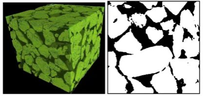
For an image with a bi-modal intensity distribution histogram, where the two peaks correspond to the solid phase and the void space respectively, thresholding might initially seem to be straightforward. However the presence of artifacts such as partial volume effects will result in a lack of accuracy. The “partial volume effect” is due to the limited resolution of the CT scan, and results in pixels with intermediate gray values appearing in the image because they merge the properties of the grain and the void space. This phenomenon can affect the segmentation results significantly as these pixels are located along the boundaries of the particles and so define the particle contacts. Image segmentation by simple thresholding gives good results when we want to separate the solid phase from the void space providing that there is enough contrast between both materials. The result is a binary image where pixels belonging to the particles have value 1 and pixels in the void space have value 0 as shown in Figure 2(b). However for the material and technology considered here simple thresholding was found to be insufficient to separate touching particles, and to define accurately the nature of the contacts. A more sophisticated segmentation technique was therefore needed and the watershed algorithm was considered.
FIGURE 2. (a) microCT image of Reigate Sand, 3D view
(b) result of simple thresholding applied to a slice.
Watershed Algorithm
The watershed algorithm is originally derived from the principle in which regions are segmented into catchment basins [6]. This analogy with a geographical model requires defining the image as a height function.
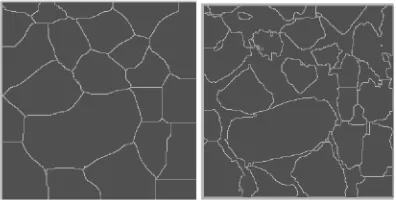
is obtained by replacing the value of the solid pixels with the value 1 by the distance, measured in pixels, to the closest void space pixel. The length of the shortest path joining any two pixels was calculated based on the Euclidean distance between them following the algorithm proposed by Danielsson [7]. Therefore, in the Euclidean distance map (EDM) the central area of each grain appears as a mountain peak, as shown in Figure 3(a).
The base for the watershed segmentation is however, the inverse of the EDM, where the topography is inverted and peaks are replaced by “minima”. A catchment basin can therefore be defined as the set of points whose path of steepest descent terminates in the same local minimum in the inverse EDM. Figure 3(b) shows the distance map after being preprocessed with a curvature flow filter available in the Insight Toolkit (an open-source software toolkit, Ibanez et al. [8]). Unlike the linear filtering, this image smoothing technique preserves the edges and the fine details remain unchanged.
FIGURE 3. (a) EDM where light pixels are high and dark
pixels are low (b) EDM after pre-filtering displayed using iso-distance contours.
There are two different watershed algorithms commonly used to distinguish particles. The first strategy is the immersion approach [9] and it consists of “flooding” the regions surrounding the minima from bottom up looking for the places where the flooded regions touch. The second “top-down” approach associates each pixel with a catchment basin by identifying a preferential downward “flow path” towards a minimum or a point that has already been associated with a minimum [10].
Immersion algorithm
The watershed segmentation was performed using MATLAB image processing toolbox [11]. This method starts with seeds at the local minima and grows regions outwards and upwards at discrete intensity levels, equivalent to a sequence of morphological operations. This limits the precision of the segmentation by imposing a set of discrete gray levels on the image.
[image:4.612.330.528.282.382.2]For the analysis presented here, the MATLAB function watershed was applied to the inverse of the distance map to produce a label matrix that contains positive integers corresponding to the locations of each catchment basin and values equal to zero along the watershed lines. However, as shown in Figure 4(a), because the watershed lines are the highest crest lines separating the regional minima, the labeled regions will not coincide with particle boundaries. Therefore the zero valued pixels (voids) in the distance map are set to a minimum value (–inf) forcing in this way the background to be its own catchment basin. The drawback of this practice is that the catchment basins will not correspond only to the solid phase but also to the void space and it will produce as many different regions as the number of unconnected areas as shown in Figure 4(b). In fact, because the void space is not associated with a unique label, it will require further consideration prior to image analysis.
FIGURE 4. Watershed ridge lines, (a) considering only
particles as catchment basins (b) both particles and void spaces are catchment basins.
Top-down approach
[image:4.612.84.286.305.404.2]merge tree. The level parameter controls the number of regions in the final labeled image by defining the precipitation that is rained into the catchment basins. As the level rises, the boundaries between adjacent regions erode and those regions merge.
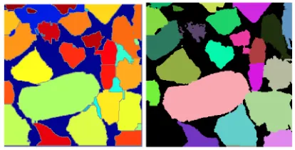
The parameters chosen for images analyzed in this investigation were threshold 0.06 and level 0.4. The results of the watershed segmentation for one slice image using both watershed approaches are shown in Figure 5(a) and Figure 5(b) respectively, and each region has associated to it a different color.
FIGURE 5. Watershed segmentation results using (a) the
immersion algorithm (b) the top-down algorithm
ANALYSIS AND DISCUSSION
The analysis of the results obtained has shown that watershed segmentation of irregular particles is a rather challenging task. One of the most common inaccuracies is image over-segmentation, i.e. the image is divided into a number of regions that is greater than the number of features that it represents.
Based on the fundamental assumption of the watershed algorithm that each regional minimum in the EDM represents the center of a distinct object, irregularities and variations along the surfaces of particles will cause the same particle to be divided into multiple parts. Pre-filtering the distance map with a smoothing filter can prevent small minor regional minima being associated with different particles. However, the basis for finding the watershed lines, i.e. lines that separate grains, is that each grain should produces a single, distinct minimum and therefore more sophisticated approaches are required. The use of marker points allows us to identify or “mark” regions that we want to be associated with one particle [13]. This can be particularly useful in the immersion algorithm considering the poor flexibility of this method. For the top-down approach, merging adjacent catchment basins based on the hierarchy of the merge tree can significantly improve the segmentation results.
There are also additional special situations. For example, consideration of elongated grains or particles with long contacts will require adapting the watershed segmentation to special rules. This will obviously
involve a good understanding of the image, and an awareness of the features of the granular material that the pixels represent [14].
CONCLUSIONS
The paper has presented a methodology for the segmentation of 3D images of granular materials exhibiting complex packing and geometries. Diverse tools and algorithms available in image processing were used and their effectiveness critically analyzed. The results have shown that automated methods for partitioning features within an image may not correspond to the same regions that a human expert would identify. Each material analyzed presented unique challenges depending on the shape, size and the need of the application. No single method can give the right answer. The tools available should be creatively combined in a constructive process to achieve the designed purpose.
ACKNOWLEDGMENTS
The authors wish to acknowledge the funding provided by Fundação para a Ciência e a Tecnologia -FCT, Portugal. Also the authors would like to thank the Department of Materials at Imperial College London in particular Professor Peter Lee, Dr. Robert Atwood and Mr. Richard Hamilton.
REFERENCES
1. T. Cuccovillo and M. R. Coop, Géotechnique 49, 6, pp. 741-760 (1999)
2. A. Cresswell and W. Powrie, Géotechnique 54, 2, pp. 107-115 (2004)
3. C. Thornton, Géotechnique 50, 1, pp. 43-53 (2000) 4. L. Cui and C. O’Sullivan Géotechnique 56, 7, pp.
455-468 (2006)
5. X. Yang, “3D Characterization of inherent and induced sand microstructure”, Ph.D. Thesis, Georgia Tech (2005) 6. J. C. Russ, “The Image Processing Handbook” CRC
Press pp. 489-496 (2007)
7. P. Danielsson, “Euclidean Distance Mapping” Comp. Graphics Image Process 14, pp. 227-248 (1980)
8. L. Ibanez, W. Schroeder, L. Ng and J. Cates, “The Itk software guide”. 2nd ed. pp. 194-207 and 524-530 (2005)
9. L. Vincent and P. Soille, IEEE Trans. Pattern Anal. Mach. Intell. 13, pp. 583–598 (1991)
10. A. P. Mangan and R. T. Whitaker, IEEE Trans. Vis. Computer Graphics 5, 4 pp. 308–21 (1999)
11. Mathworks, Image Processing Toolbox 7.0 (2004) 12. J. E. Cates, R. T. Whitaker and G. M. Jones Medical
Image Analysis 9 pp. 566–578 (2005)
13. P. Soille, “Morphological Image Analysis” Springer pp. 267-290 (2003)
[image:5.612.83.290.183.288.2]