Research in Layer Identification

Qualifying Exam

Jerome E. Mitchell

Abstract

In order to satisfy qualifying exam requirements adhered to by the School of Informatics and Computing, I will provide an overview of related and work in layer identification and explain

Introduction

Related Literature

There has been relatively little work on estimating near surface internal layers from echograms acquired in either Greenland or Antarctica. Most related work has focused on identifying either basal boundaries or other coarse properties of echograms. For example, Freeman et al. [1] and Ferro and Bruzzone [2] investigated how shallow ice features can be automatically detected in icy regions from echograms of Mars. In other work, Ferro and Bruzzone [3] used echograms of the Martian subsurface to detect basal returns. Approaches to identifying surface and bedrock layers in polar radar imagery have been addressed in Reid et al. [4], Ilisei et al. [5], and Crandall et al. [6].

Near Surface Internal Layers

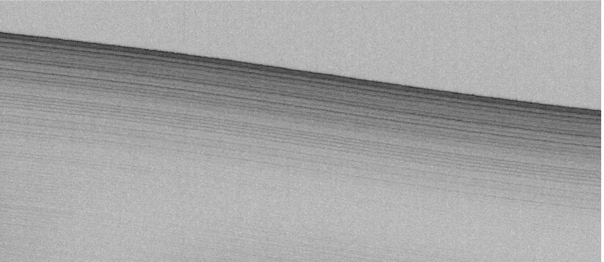
We used observations about how domain experts detect layer boundaries in order to develop a semi-automated algorithm to mimic these behaviors. As shown in Figure 1a and as is typical for our experimental images, the surface reflection is very strong and near surface layer intensity generally decreases as depth increases. Also, near surface layers are approximately parallel, but may have modest changes in slope both to one another

and to the ice surface. We proposed a technique, which attempts to find the

prominent surface reflection and searches for similar

(but invariably weaker) layer

structures below the surface. We used each layer as an estimate of the appearance

for the layer below it and an active contours (“snakes”) model to snap the correct

layer structure given this estimate. We describe the process of detecting the

surface, estimating layer location using curve point classification and refining the

use of snakes in the following sections:

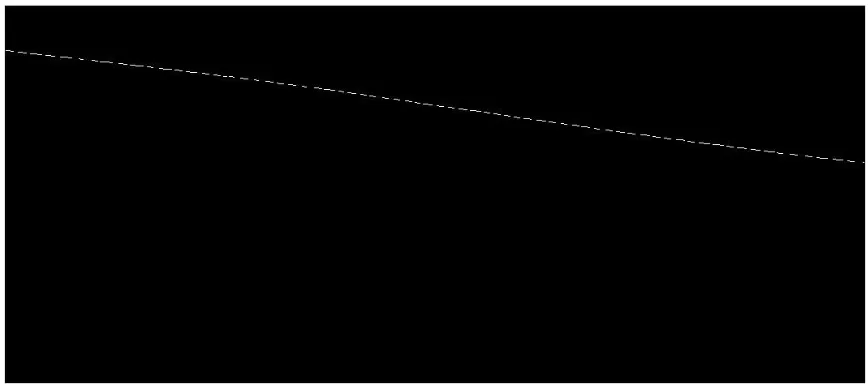
To find the location of the surface boundary, which is typically the most

prominent edge in the echogram, we used a Canny edge detector [10] because of

its performance in detecting strong intensity contrasts for our near surface layer

dataset (shown in Figure 2). In detecting this initial ice surface, the following fixed

Canny parameters were used: a sigma of 2 for the standard deviation of the

Gaussian filter and a low and high thresholds of 0.7 and 1.8, respectively. Since

the ice surface is symmetrical to subsequent layers, it provides a good starting

template.

Figure 2: Canny Edge Detector of Ice Surface

Curve Point Classification

While the ice surface can be readily detected by edge detection, using it for near

surface internal layers is not possible because of the very weak layer boundaries

and the noise inherent in echograms. As a consequence, we used Steger’s

likely to be part of curvilinear structures. In short, this approach computes

statistics on gradient structures within local image patches and investigates areas

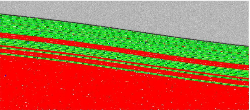
with prominent gradients in a coherent direction. We identified peaks for scores

computed by Steger (shown as blue asterisks in Figure 3b) and used these to

suggest initial curve positions for estimating near surface internal layers. For the

first layer, we used the ice surface estimated previously and shifted it down, (in the

y direction) so it intersected the first maximum point. This process was repeated

until the number of near surface internal layers specified by the user has been

found and gave initial estimates of layer positions and shapes, which we refined in

the next step.

Figure 3b: Detected Layers (green) and Maximum Curve Points (blue asterisks)

Active Contours

To refine the curve shape and position estimates from the previous section, we used an active contours (snakes) model [12], a procedure for allowing an initial contour to gravitate towards an object boundary. Briefly summarized, the snakes model defines an energy function, which computes the “cost” of a particular curve (sequence of points). The function is defined to encourage the curve to align with high-gradient edge

pixels

but to discourage the curve from having either discontinuities or sharps bends.

These two goals are often in tension, and the energy minimization function is used

to find the curve with the best trade-off between them. An iterative gradient

descent (hill-climbing) algorithm is used to find the curve with the best (local)

minimum, given an estimate of the correct answer as initialization. In our

methodology, active contours are used to warp the initial templates from the last

to succeed, the initial contour must be close to the actual layer in order for the

snake to find the correct boundary and not be confused by either noise or other

edges in the image. A layer is fit when the energy function converges to a either

minimum or when a maximum number of iterations has reached its threshold.

Using active contours requires setting several parameters (α,

β, and

γ values -

these are weights on the terms in the energy minimization function and control the

tradeoff between the forces mentioned above). We tuned these parameters

empirically to find values, which work well on most images and allow the user to

further tune them on a per-image basis, if needed.

Results

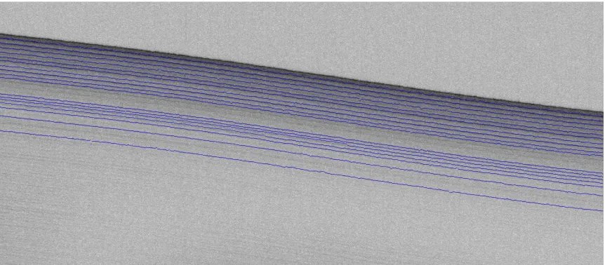
Figure 4 shows the result of our approach for Figure 1. We observe it has successfully found over a dozen layers correctly, although it misses some of the very faint layers towards the bottom of the echogram.

Conclusions

We have developed a semi-automated approach to estimate near surface internal layers in snow radar imagery. Our solution utilizes an active contour model in addition to edge detection and Steger’s curve classification. Our technique is a step towards the ultimate goal of unburdening domain experts from the task of dense hand selection. By providing tools to the polar science community, high resolution accumulation maps can be readily processed to determine the contribution of global climate change to sea level rise.

References

[1] G. Freeman, A. Bovik, and J. Holt, “Automated detection of near surface Martian ice layers in orbital radar.

[2] Ferro and L. Bruzzone, “Automatic extraction and analysis of ice layering in radar sounder data,” IEEE Transactions on Geoscience and Remote Sensing, 2013.

[3] A. Ferro and L. Bruzzone, “Analysis of radar sounder signals for the automatic detection and characterization of subsurface features,” IEEE Transactions on Geoscience and Remote Sensing, 2012.

[5] A.-M. Ilisei, A. Ferro, and L. Bruzzone, “A technique for the automatic estimation of ice thickness and bedrock properties from radar sounder data acquired at Antarctica,” in IEEE International Geoscience and Remote Sensing Symposium, 2012, pp. 4457–4460. [6] D. Crandall, G. Fox, and J. Paden, “Layer-finding in radar echograms using probabilistic graphical models,” in International Conference on Pattern Recognition, 2012, pp. 1530–1533.

[7] M. Fahnestock, W. Abdalati, S. Luo, and S. Gogineni, “Internal layer tracing and age depth-accumulation relationships for the northern greenland ice sheet,” Journal of Geophysical Research, vol. 106, no. D24, pp. 33789–33, 2001.

[8] N. Karlsson and D. Dahl-Jensen, “Tracing the depth of the holocene ice in north greenland from radio-echo sounding data,” Annals of Glaciology, 2012.

[9] L. Sime, R. Hindmarsh, and H. Corr, “Instruments and methods automated processing to derive dip angles of englacial radar reflectors in ice sheets,” Journal of Glaciology, vol. 57, no. 202, pp. 260–266, 2011.

[10] J. Canny, “A computational approach to edge detection,” IEEE Transactions on Pattern Analysis and Machine Intelligence, no. 6, pp. 679–698, 1986.

[11] C. Steger, “An unbiased detector of curvilinear structures,” IEEE Transactions on Pattern Analysis and Machine Intelligence, vol. 20, no. 2, pp. 113–125, 1998.