Research on the Hedging of CSI300 Stock Index Future
Based on VaR and CVaR Model
Zijian Xu1, Benshan Shi, Sheng Zhou2 1
Emeixiaoqu accounting department, Southwest Jiaotong University, Emei, Sichuan, 610031, China
2
School of Economic and Management, Southwest Jiaotong University, Chengdu, Sichuan, 610031, China
Abstract. Hedging function is one of the most significant functions of stock index futures, and it received extensive public attention. This article set VaR and CVaR as hedging objective function of the hedging model in China and proposed the hedging effect measurement method based on VaR and CVaR. It also used the actual data of CSI300 stock index future to calculate its hedging effect. It is found from the result that the hedging model of stock index future based on VaR and CVaR can effectively reduce the risk of portfolio, and a relatively good accumulated income rate will be obtained. By comparison, the hedging model of stock index future based on CVaR will do better in controlling the risk of portfolio, while the hedging model of stock index future based on VaR will obtain a better accumulated income rate.
Keywords. stock index future; hedging; VaR; CVaR
1 Preface
The hedging function is a core function of futures market, and also the premises for the development of futures market. Hedging refers to the action that a trader purchases or sells the futures contract with the same type and quantity of traded goods but with different orientation, expecting to compensate for the actual price risk due to price change in the spot market by selling or purchasing the futures contract sometime. In April 16, 2010, China formally released CSI300 stock index future based on CSI300 index. Its release realized short sale in Chinese stock market. The investor may hold the spot stock while short selling the stock index future to achieve the hedging purpose and effectively avoid the systematic risk in the market.
The current researches on the hedging rate of stock index future are mainly divided into two types: The first type of model research is based on the minimization of portfolio risk. This model gets the best hedging ratio of portfolio by minimizing the certain risk functions. These particular risk functions include variance[3], downside risk[6,11], MEG[2], etc.. The second type of model research is based on the hedging ratio with greatest utility.This model gets the best hedging ratio[1,8] by maximizing the utility function[1,8].
The standard to measure the assets risk by fluctuation rate, namely the variance, is widely used in the risk measurement for assets, but this kind of method to measure the assets risk with symmetric profit and loss is contradictory to the feelings of investors for the risk. In the actual
7KLVLVDQ2SHQ$FFHVVDUWLFOHGLVWULEXWHGXQGHUWKHWHUPVRIWKH&UHDWLYH&RPPRQV$WWULEXWLRQ/LFHQVHZKLFKSHUPLWV DOI: 10.1051/
C
Owned by the authors, published by EDP Sciences, 2015
/2 01
investment, the investor only faces the risk related to loss, so a reasonable risk measurement method shall be solely related to the investment loss, which is the main idea of method design for Value at Risk (hereinafter referred to as VaR). VaR method is currently one of the most widely used tools for risk measurement in risk management. It overcomes the defect in the traditional variance that has symmetric loss and profit, and focuses more on the trailer distribution that causes loss. The CVaR model is a certain extent, can overcomes several defects in VaR. There are some scholars at home and aboard who have used VaR and CVaR model to conduct research on the heading of futures and obtained helpful conclusion [4.5, 9-12].
This article will take VaR and CVaR as the method to measure the portfolio risk, and take the minimum of VaR and CVaR risk as the objective function to establish the hedging model. It will also take CSI300 stock index future as the research objective to calculate the best hedging ratio of CSI300 stock index future and conduct empirical analysis on the efficiency of hedging. Wish that it would boost the development of Chinese stock index future market.
2 Principle of hedging based on VaR and CVaR
2.1 Calculation of hedging ratio based on the minimum of VaR
(1) Definition and estimation method of VaR
VaR refers to the maximum of loss the portfolio may suffer. In the actual calculation process, its measurement may be based on the income rate and income value (or other indexes as the measurement standards). Its expression is as follows:
prob(
R
VaR
)
(1) Where, R refers to the loss ratio of assets in the holding period, and VaR refers to the value at risk when the confidence level is within1
. VaR is a positive value here. The risk measurement VaR may be related to the preference of the broker. The broker that dislikes the risk may choose a relatively high confidence level. The higher confidence level will lead to larger VaR, but lower probability.There are many estimation methods for VaR, and different estimation methods will get varied distributions. Currently, there are mainly three calculation methods for VaR: parameter method, historical simulation method and Monte Carlo simulation method. This article used parameter method for the calculation of VaR. The calculation formula of VaR may be obtained by calculation:
1
( )
VaR
(2)
(2) Calculation of the best hedging ratio
This article deduced the calculation of the best hedging ratio for portfolio, and the detailed parameters and the parameter meanings are as follows:
p refers to the average of income rate ofportfolio;
s refers to the average of income rate of spot index; f refers to the continuousincome rate of stock index future in current month;
prefers to the standard deviation of incomerate of portfolio;
s refers to the standard deviation of spot index; f refers to the continuousincome rate of future index and of spot index;
sf refers to the correlation coefficient for the income rate of future index and of spot index; refers to the confidence level;1
( )
refers to the inverse function of standard normal distribution function as the confidence level is ;
h
refers to the best hedging ratio.The expression of VaR for portfolio that may be obtained according to the average and variance of portfolio is as follows:
1 2 2 2
( )
s2
sf f s fVaR
h
h
h
(3)
Solve the formula (3), and two values may be obtained. The best hedging ratio can be determined by comparing the VaR corresponding to those two values. The resulting best hedging ratio is as follows:
2 2 2 2
2 2
2 2 2 1 2 1 2 2
1
( )
( )
sf t
f f f
f s
sf f s f s
VaR t
f f f f f
h
(4)
2.2 Calculation of hedging ratio based on the minimum of CVaR
Conditional Value at Risk (hereinafter referred to as CVaR), also called Mean Excess Loss, refers to the expected value exceeding the loss of VaR. Please see Rockafellar and Uryasev [10] for more. It refers to the investor’s expected value for
1
section in the income distribution in a certain time t and a certain confidence level. The expression is as follows:CVaR
E R R
( |
VaR
)
(5)CVaR refers to the conditional mean with its loss exceeding VaR. It represents the average level of excess loss and reflects the average potential loss that may be suffered when the loss exceeds VaR. Assuming R complies with normal distribution; the formula (5) is converted as follows:
CVaR
E
R
|
R
VaR
(6) Set
R
x
, and x will comply with standard normal distribution.( )
x
refers to probability density function for standard normal distribution, and:1
( )
( )
CVaR
x x dx
(7)
To simplify the formula, set:
1( )
( )
x x dx
C
(8)Further calculate
C
in formula (8), we get:2 1( )
The confidence level
is a constant, so1
( )
is a constant, and
C
mentioned informula (11) is also a constant. CVaR in the confidence level
will be obtained asC
is used to represent the corresponding variant in formula (6):CVaR
C
(10)Then, the best hedging ratio is calculated as follows:
2 2 2 2
2 2 2 2 2 2 2 2
1
sff f f
f s
sf f s f s sf
CVaR sf
f f f f f
h
C
C
(11)
2.3 Inspection of hedging validity
(1) Measurement of hedging validity based on variance
Traditionally, the best hedging ratio is calculated in the assumption that the variance is in its minimum value. So in the inspection of hedging efficiency, we mainly compare the reduction percentage between the variance of income rate of portfolio after hedging and the variance of assets that are not hedged, as shown in formula (12).
2 2
2 s
s
p
HE
(12)(2) Measurement of hedging validity based on VaR and CVaR
This article took the minimum of VaRand CVaR as the objective function to calculate the best hedging ratio for portfolio, so in the inspection of hedging efficiency, the reduction percentage of VaR of portfolio after and before the hedging is used to measure the effect of hedging:
* s p
s
VaR
VaR
HE
VaR
(13)In the above formula,
VaR
s refers to VaR of income rate of spot index, andVaR
p refers toVaR of income rate of portfolio after hedging. Similarly, a hedging measurement model based on CVaR will be obtained from the above formula.
(3) Accumulated income rate
Establish the portfolio by respectively taking the minimum of variance, VaR and CVAR as the objective functions, and compare the accumulated income rate of portfolio for different objective functions to measure the effect of hedging.
3 Analysis based on the data of CSI300 stock index future
In this chapter, an empirical calculation will be conducted according to the actual data of CSI300 index and CSI300 stock index future, so as to inspect the validity of calculation model of the best hedging ratio based on the minimized objective of VaR and CVaR.
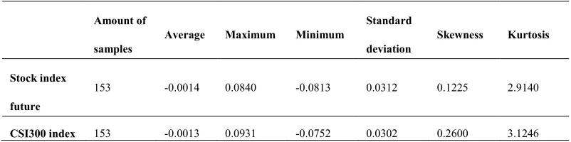
In the empirical calculation, the income rate of spot portfolio will be replaced by the income rate of CSI300 index, and the data of weekly income rate of CSI300 index and the data of continuous weekly income rate of CSI300 stock index future will be selected as the research data. As it is not a short-term action to use the hedging, using the data of weekly income rate in the empirical research will be more compliant with the actual situation; In this chapter, the parameter method will be used to calculate the VaR and CVaR of portfolio, and the income rate will affect the significance of calculation result, for example, the comparability of result generated by calculating the daily income rate will be worse. As for the data n the research period from April 19, 2010 to April 19, 2013, 3 years, 153 weeks in total, the descriptive statistic feature of the data is as shown in Table 1:
Table 1. Descriptive statistics of weekly income rate of future and spot index
Amount of
samples
Average Maximum Minimum
Standard
deviation
Skewness Kurtosis
Stock index
future
153 -0.0014 0.0840 -0.0813 0.0312 0.1225 2.9140
CSI300 index 153 -0.0013 0.0931 -0.0752 0.0302 0.2600 3.1246
The amount of samples in the research period is 153; The average of income rate of CSI300 index
s=-0.0013; The standard deviation s=0.0312; The maximum weekly income rate within the research period is 0.0840; The maximum weekly loss rate is -0.0813; The average of income rate of CSI300 stock index future f =-0.0014; The standard deviation s =0.0302; The maximum weekly income rate within the research period is 0.0931; The maximum weekly loss rate is -0.0931; The correlation coefficient for the income rate of future index and of spot index will be obtained by calculation, namely sf =0.9755, indicating that the correlation degree of the weekly income rate of future index and spot index is very high.3.2 Best hedging ratio based on VaR and CVaR
The value of quantile
1
( )
in different confidence levels will be obtained by reference to the
form, and the value of
C
in different confidence levels will be obtained by calculation according to formula (9), as shown in Table 2:Table . Quantiles in different confidence levels
Confidence level 99.0% 97.5% 95.0%
1
( )
2.3263 1.95996 1.6449
C
2.6652 2.3378241 2.0627As shown in Form 2, with the reduction of confidence level, the value of quantile
1( )
under the standard normal distribution will be gradually reduced, so do the value of
C
, but with less reduction compared to 1( )
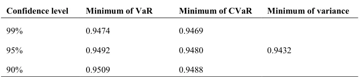
.Table 3 shows the calculation result of the best hedging ratio that takes VaR and CVaR as the objective functions in different confidence levels:
Table 3. Best static hedging ratio in different confidence levels
Confidence level Minimum of VaR Minimum of CVaR Minimum of variance
99% 0.9474 0.9469
0.9432
95% 0.9492 0.9480
90% 0.9509 0.9488
According to the calculation result of the best hedging ratio in different confidence levels shown in Table 3, it is found that the best hedging ratio that takes VaR as the objective function will be increased with the reduction of confidence level, and the calculation result of the best hedging ratio that takes CVaR as the objective function has the same phenomenon, but with less increasing rate compared to that which takes VaR as the objective function. As in the research period, the average of weekly income rate of future index is negative, and the values of quantiles, namely
1
( )
and
C
, are both in the denominator, its value will be gradually decreased with the reduction of confidence level, so that the calculated best hedging ratio will be gradually increased. [image:6.482.65.413.361.564.2]The VaR and CVaR of portfolio after hedging in different confidence levels will be calculated according to the calculation result of the best hedging ratio in different confidence levels shown in Table 3 and according to formula (2) and formula (10). It is as shown in Table 4:
Table 4. VaR and CVaR of portfolio after hedging in different confidence levels
VaR as the objective function
Confidence level Average Standard deviation VaR CVaR
99% 6.63E-05 0.006644 -0.015522 -0.017774
95% 6.89E-05 0.006645 -0.010999 -0.013776
90% 7.13E-05 0.006647 -0.00859 -0.011737
CVaR as the objective function
Confidence level Average Standard deviation VaR CVaR
99% 6.56E-05 0.006644 -0.015522 -0.017773
95% 6.71E-05 0.006645 -0.010997 -0.013774
90% 6.83E-05 0.006645 -0.008585 -0.011730
level, the average income of portfolio after hedging will be gradually increased and the standard deviation will be gradually decreased, because the value of VaR and CVaR is related to the confidence level. As the confidence level is reduced, the value of VaR and CVaR will be reduced accordingly. When CVaR is taken as the objective function, the value of VaR and CVaR of portfolio after hedging will be lower than that when VaR is taken as the objective function.
[image:7.482.106.377.160.220.2]To compare the validity of hedging, we conduct calculation to obtain the VaR and CVaR of CSI300 index in different confidence levels, as shown in Table 5:
Table 5. VaR and CVaR of CSI300 index in different confidence levels
Confidence level 99% 95% 90%
VaR -0.068904 -0.04834 -0.037376
CVaR -0.079132 -0.060949 -0.051663
3.3 Inspection of hedging validity
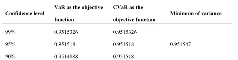
Inspect the validity of hedging that takes VaR and CVaR as the object function according to the reduction amplitude of variance and reduction degree of VaR and CVaR, as shown in Table 6 and Table 7:
Table 6. Hedging validity-reduction of variance
Confidence level
VaR as the objective
function
CVaR as the
objective function
Minimum of variance
99% 0.9515326 0.9515326
0.951547
95% 0.951518 0.951518
90% 0.9514888 0.951518
According to the measurement index of hedging validity proposed by Ederitong[3], namely the formula (12) of reduction percentage about the comparison of variance of portfolio after and before hedging, the calculation result is as shown in Table 6.The hedging that takes VaR and CVaR as the objective function can also do well in reduction of portfolio variance, and adjust the reduction amplitude of variance according to the change in the confidence level, namely it can adjust the risk level to a certain extent. While the risk level will be a fixed value if the hedging takes the minimum of variance as the objective function. It indicates that the hedging that takes VaR and CVaR as the objective function will be valid if the reduction percentage of variance is taken as the measurement index of hedging validity.
This article takes VaR and CVaR as the objective function of hedging, so it has a theoretical and practical meaning to take the reduction percentage of VaR and CVaR of portfolio after and before hedging as the measurement index of hedging validity. Respectively calculate the value of VaR and CVaR of portfolio after and before hedging when VaR and CVaR are taken as the objective function of hedging, and get the value of
HE
*according to the formula (13). The result is shown in Table 7. [image:7.482.52.437.321.419.2]of VaR and CVaR for hedging of stock index future that takes CVaR as the objective function will be better than that which takes VaR as the objective function, indicating that according to the reduction percentage of VaR and CVaR, the portfolio that takes CVaR as the objective function will do better in risk reduction.
Table 7. Hedging validity of stock index future- Reduction percentage of VaR and CVaR
VaR as the objective function CVaR as the objective function
Confidence level VaR CVaR VaR CVaR
99% 0.7747 0.7754 0.7747 0.7754
95% 0.7725 0.7740 0.7725 0.7740
90% 0.7702 0.7728 0.7703 0.7729
3.4 Accumulated income rate
[image:8.482.35.441.332.433.2]Then, this article will make an analysis on the accumulated income rate of portfolio after and before hedging to inspect the accumulated income rate of portfolio after and before hedging as it takes VaR and CVaR as the objective function.
Table 8. Accumulated income rate in different objective functions (%)
Confidence
level
VaR as the
objective function
CVaR as the
objective function
Minimum
of variance
Stock index
future
CSI300 index
99% 0.68% 0.67%
0.59%
95% 0.72% 0.69% -25.55% -23.53%
90% 0.76% 0.71%
Table 8 shows the accumulated income rate of portfolio after hedging in different objective functions. Either VaR, CVaR or the minimum of variance is taken as the objective function; the positive accumulated income rated will nevertheless be obtained. While in the same period, the accumulated income rate of CSI300 index is -23.53%, and -25.55% for CSI300 stock index future. By comparing the accumulated income rate of portfolio after hedging in different objective functions, the accumulated income rate of portfolio that takes VaR and CVaR as the objective function will be better than that which takes the minimum of variance as the objective function, and can adjust the accumulated income rate according to the change in confidence level. Furthermore, the portfolio after hedging that takes VaR as the objective function has the largest accumulated income rate.
4 Conclusion
There are three conclusions from the empirical result: (1) The hedging model of stock index future based on VaR and CVaR can efficiently reduce the risk of portfolio; (2) All the established portfolios have a relatively desirable accumulated income rate compared to the stock market in the same period; (3) By comparing those two models, the hedging model of stock index future based on CVaR will do better in controlling the risk of portfolio, while the hedging model of stock index future based on VaR will have a better accumulated income rate.
Acknowledgement
The basic research funding to central’s university (2682014BR015EM). The research supporting projects to High-level scholar team construction support by Southwest Jiaotong University-Emei (RC2013-26).
References
1. Cecchetti, S.G., Cumby, R.E., Figlewski, S. Estimation of the optimal futures hedge [J]. Review of Economics and Statistics, 1988, 70(4): 623-630.
2. Chen, S.S., Lee, C.F., Shrestha, K. Futures hedging ratios: a review [J]. The Quarterly Review of Economics and Finance, 2003, 43(3): 433-465.
3. Ederington, L.H. The hedging performance of the new futures markets [J]. Journal of Finance, 1979, 34(1): 157-170.
4. Gordon, J.A., Alexandre, M.B. A comparison of VaR and CVaR constraints on portfolio selection with the Mean Variance model [J]. Management Science, 2004, 50(9): 1261-1273. 5. Huang, J.C., Chiu, C.L., Lee, M.C. Hedging with zero-value at risk hedge ratio [J]. Applied
Financial Economics, 2006, 16(3): 259-269.
6. Kahneman D., Tversky A. Prospect Theory: An Analysis of Decision under Risk [M]. Econometrica, 1979: 263-291.
7. Krokhmal P., Palmquist, J., Uryasev S. Portfolio optimization with conditional value-at-risk objective and constraints [J]. Journal of Risk, 2002(4):43-68.
8. Lence, S.H .Relaxing the assumptions of minimum-variance hedging [J]. Journal of Agricultural and Resource Economics, 1996, 21(1): 39-55.
9. Richard, D.H., Shen, J. Hedging and value at risk [J]. Journal of Futures Markets, 2006, 26(4): 369-390.
10. Rockafellar, R. T., Uryasev, S. Optimization of Conditional Value-at-Risk [J].Journal of Risk, 2000(2): 21-41.
11. Tversky, A., Kahneman, D. Advances in Prospect Theory: Cumulative Representation of Uncertainty. Journal of Risk and Uncertainty, 1992, 5: 297-323.
12. Chi, G.T., Zhao, G.J., Yang Z.Y., Best Hedging Ratio Model of Future Based on CVaR and Its Application [J]. Journal of Systematic Management, 2009, 2: 27-33.