Power Aware Scheduling of Virtual Machines in DVFS enabled Clusters

Power-Aware Scheduling of Virtual Machines in

DVFS-enabled Clusters

Gregor von Laszewski

, Lizhe Wang

, Andrew J. Younge

, Xi He

†

Pervasive Technology Institute, Indiana University at Bloomington

2729 E 10th St., Bloomington, IN 47408

‡

Service Oriented Cyberinfrastructure Lab, Rochester Institute of Technology

Blg 74, Lomb Memorial Dr., Rochester, NY 14623

Abstract—With the advent of Cloud computing, large-scale virtualized compute and data centers are becoming common in the computing industry. These distributed systems leverage commodity server hardware in mass quantity, similar in theory to many of the fastest Supercomputers in existence today. However these systems can consume a cities worth of power just to run idle, and require equally massive cooling systems to keep the servers within normal operating temperatures. This produces

CO2 emissions and significantly contributes to the growing environmental issue of Global Warming. Green computing, a new trend for high-end computing, attempts to alleviate this problem by delivering both high performance and reduced power consumption, effectively maximizing total system efficiency.

This paper focuses on scheduling virtual machines in a compute cluster to reduce power consumption via the technique of Dynamic Voltage Frequency Scaling (DVFS). Specifically, we present the design and implementation of an efficient scheduling algorithm to allocate virtual machines in a DVFS-enabled cluster by dynamically scaling the supplied voltages. The algorithm is studied via simulation and implementation in a multi-core cluster. Test results and performance discussion justify the design and implementation of the scheduling algorithm.

Keywords - Dynamic Voltage and Frequency Scaling; Cluster Computing; Virtual machine; Scheduling

I. INTRODUCTION

Modern high-end computing can provide high performance computing solutions for scientific and engineering applica-tions. However, today’s high performance computers consume tremendous amounts of energy. For example, a 360-Tflops supercomputer (such as IBM Blue Gene/L) with conventional processors requires 20 MW to operate, which is approximately equal to the sum of 22,000 US households power consumption [1], [2]. Furthermore, it is estimated that servers consume 0.5 percent of the world’s total electricity usage [3], which if current demand continues, is projected to quadruple by 2020. Unfortunately, the computing system temperature may in-crease rapidly due to inefficient cooling equipments. Based on Arrhenius time-to-fail model [4], every 10◦C increase of temperature leads to a doubling of the system failure rate. Hence, it is obvious that power-aware resource management for high end computing is highly desirable. Dynamic voltage and frequency scaling (DVFS) [5] is an efficient technology to control the processor power consumption. With aide of support technologies such as Intel SpeedStep and AMD PowerNow!, modern processors can be operated in several frequencies with different supply voltages.

Virtual machine technology is adopted for high end com-puting to achieve efficient comcom-puting resource usage. Some technical work has reported that virtual machine could be used for scientific applications with tolerable performance punishment [6], [7]. A virtual machine (VM) is a software based machine emulation technique to provide a desirable, on-demand computing environments for users. As documented in [8], [6], [9], virtual machine provisioning is a popular part of cluster deployments. The normal process of a cluster operating with the use of virtual machines for executing jobs is shown as follows:

1) A compute cluster provides various virtual machine templates.

2) When a job arrives at the cluster, the cluster scheduler allocates the job with a preconfigured virtual machine then starts it on proper compute nodes.

3) The job is executed in the virtual machine.

4) After the job is executed, the virtual machine is shut-down.

virtual machines for a DVFS-enabled cluster. The scheduling algorithm is specified in detail in Section V. Section VI renders a real implementation of the scheduling algorithm and evaluates a multi-core cluster system. Section VII discusses a simulator for the scheduling algorithm, the simulation results and performance evaluation of the scheduling algorithm. Fi-nally Section VIII concludes the paper and point out future work.

II. RELATEDWORK

This paper provides a novel power-aware scheduling al-gorithm for virtual machines in clusters. Therefore, related work in both frequency and voltage scaling, cluster computing, and virtual machine technologies need to be addressed and evaluated.

A. Power-Aware Cluster Computing

Dynamic voltage and frequency scaling (DVFS) is an effec-tive technique to reduce processor power dissipation [11], [12]. By lowering processor clock speed and supply voltage during both idle times and compute intensive application phases, large reductions in power consumption can be achieved with modest performance loss. High-end computing communities, for example, cluster computing and supercomputing in large data centers, have applied DVFS techniques to reduce power consumption and achieve high reliability and availability [13], [14], [15], [16]. A power-aware cluster is defined as a compute cluster where compute nodes support multiple power/perfor-mance modes, for example, processors with frequencies that can be turned up or down. Current technologies exist within the CPU market such as Intel’s SpeedStep and AMD’s Pow-erNow! technologies. These dynamically raise and lower both frequency and CPU voltage depending on system load using ACPI P-states [17]. Popular DVFS-based software solutions for high end computing include:

• A scientific application is modeled with DAG and the critical path is identified in for the application. Then it is possible to reduce the processor supply voltage during non-critical execution of tasks [18].

• Parallel applications are identified with different exe-cution phase, in contrast to compiler or other system level software schedules proper processor voltage and frequency for different execution phases [19].

• Some implementations [20] build an online,

performance-driven runtime system to automatically scale processor voltages.

The first two methods normally require prior knowledge of applications with aides benchmarking and profiling. The third method is based on a runtime algorithm and schedule jobs dynamically with no prior information of running applications.

B. Virtual Machine-Based Computing

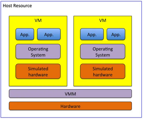
A VM is a software artifact that executes other software in the same manner as the machine for which the software is developed and executed [21]. This is typically achieved using a hypervisor or Virtual Machine Monitor (VMM) in between

the harware level and the operating system level to abstract the hardware and enable the use of multiple, concurent operating systems. Figure 1 shows a host resource that provides two virtual machines via the VMM support software.

VM
 VM


VMM


Hardware
 Simulated


hardware
 Opera3ng



System


App.
 App.


Simulated
 hardware
 Opera3ng



System


App.
 App.


Host
Resource


Fig. 1. Virtual Machine Concept

In general, cluster computing can benefit from virtual ma-chines in the following aspects [22].

• On-demand creation and customization:Virtual machine administrators can create and customize virtual machines, which can provide specific required resource provisioning for users e.g., operating system, memory, storage, etc.

• Legacy system support: Virtual machines can support both legacy software and entire legacy computing en-vironments, including hardware, operating system, and applications, by on-demand creation of user-preferred virtual machines.

• Administration privileges and site autonomy: Users of virtual machines could obtain administrative privileges if each user of the hosting resources is allocated a virtual machine. This scenario alleviates the task of system administrator and gives flexibility for application users. As virtual machine can be started, shutdown and migrated dynamically, it is therefore easier to manage virtual machines in a computing center than a large amount of jobs. The computing center that provides virtual machine also can keep the site autonomy. For example, computing center is free from supporting software licenses to users.

• Performance isolation: Virtual machines can guarantee

the performance for users and applications. Applications executed in virtual machines would not find the per-formance perturbation, which is invoked by simultane-ous usage of multiple applications on traditional multi-programmed computers.

III. SAMPLEUSAGESCENARIO

This section provides a typical cluster (IKEP cluster) opera-tion scenario [8], [6] of virtual machines based on the WLCG applications, for example, in the computer center of University Karlsruhe. The Worldwide LHC Computing Grid (WLCG) [23] is a global collaboration of more than 2000 physicists of 182 institutes of 38 nations. One example of a typical institute cluster is the IEKP Linux cluster, which consists of 40 compute nodes (x86-64 based architecture), 5 file servers with a total capacity of 20 TB and 6 portal machines for software development. The situation at the IEKP is also typical because it serves three different groups which work on different large-scale international projects (CDF [24], CMS [25] and AMS [26]), each having different software and different comput-ing requirements. The IKEP cluster has to balance different requirements of software/hardware configuration for various jobs from different projects. Even if an agreement is achieved by multiple projects, it is still hard to configure computing environments for High Energy Physics (HEP) computing. For example, tens of hours are required to compile, install and configure CMS computing environments.

!"# !"#

$%"&'()# *%+)# !"#

$%"&'()#*%+)#

!"#

,-.)#

/)0!)0# 1)2+#*%+)# !"#

!"#

3%4#

#####5(20(#2#!"# 67)8'()#3%4#-*#2##!"#

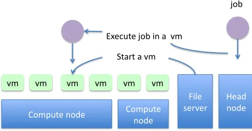
Fig. 2. Sample Usage of IKEP Cluster

Therefore, virtual machines are deployed to execute incom-ing jobs. There is a file server to provide virtual machine templates. All typical jobs from WLCG, CDF, CMS, and AMS are preconfigured in virtual machine templates. When a job arrives at the head node of the IKEP cluster, a correspondent virtual machine is dynamically started on certain compute node at IKEP cluster to execute the job (see Figure 2).

With the concrete background of virtual machine based cluster computing and the DVFS technology, next section formally define the system models and research issues of scheduling a DVFS-enabled cluster.

IV. SYSTEMMODEL

This section provides the formal description for a DVFS-enabled cluster, virtual machine jobs, and performance models, which are employed as basis of the formal problem definition in Section IV-D and the scheduling algorithm in Section V.

A. Performance Model

A DVFS-enabled cluster contains multiple compute nodes. It is assumed that each compute node can be operated in

mul-tiple voltage with different frequencies. We define a operating pointopj as follows:

opj = (vop, sop) (1)

Where,

opj is the j-th operating point;

vop is the processor operating voltage ofopj;

sop _{is the processor operating frequency ofop} j;

vmin=op1.vop< op2.vop< ... < opJ.vop=vmax;

smin=op1.sop< op2.sop< ... < opJ.sop=smax;

1≤j ≤J,J is the total number of operating point.

Therefore a set of operating points for a DVFS-enabled processor, OP, is defined as:

OP = [

1≤j≤J

{opj} (2)

The energy consumption of modern processor, E, can be divided into two parts, dynamic energy consumption

Edynamic, and static energy consumption Estatic [27]:

E=Edynamic+Estatic (3)

According to [28], the dynamic power consumptionPdynamic

is computed as follows:

Pdynamic=ACv2s (4)

Where,

Ais the percentage of active gates;

C is the total capacitance load;

v is the supply voltage;

sis the processor frequency.

Then, we have:

Edynamic=

X

t

Pdynamic· 4t (5)

where,

Pdynamicis the dynamic power;

4t is a time period.

Estatic is normally proportional toEdynamic [29], [30]:

Estatic∝Edynamic (6)

Therefore the whole power consumption could be estimated as follows [27]:

E∝Edyanmic (7)

In conclusion, we have the performance model:

E∝X

t

v2·s· 4t (8)

Where,

v is the processor operating voltage during4t;

sis the processor operating frequency during4t;

B. Compute Cluster Model

A commodity cluster typically contains multiple compute nodes, which are formally termed as Processing Elements (PEs) in a general parallel computing context. In this paper we focus on the study of homogeneous clusters: all PEs inside the cluster have the same processor speed or provide identical processing performance in term of MIPS (Million Instruction Per Second). A homogeneous cluster, C, therefore can be formally described as follows.

The k-th PE is defined as

pek = (oppe, vpe, spe) (9)

Where,

pek is the k-th PE inside a cluster C;

oppe is the operating point of pek; vpe is the processor

operating voltage of pek;

spe is the processor operating frequency of pek;

1≤k≤K,K is the total number of PEs.

Hence, a cluster C is defined by its set of processing elements

C= [

1≤k≤K

{pek} (10)

C. Virtual Machine Model

Normally users submit virtual machine requests to popular virtual machine management systems with QoS requirements, such as required virtual processor speed, memory size, storage size, operating system and other hardware/software environ-ments.In the context of power-aware scheduling, we model a virtual machine in terms of required processor frequency and required execution time. Each virtual machinevmi is defined

as

vmi= (sr,∆t, tr) (11)

where,

vmi is thei-th virtual machine to be scheduled;

sr _{is the required processor speed forvm} i;

∆t is the required execution time ofvmi;

tr is the required starting time ofvmi;

1≤i≤I,Iis the total number of incoming virtual machines. Hence, the set of all virtual machines is defined by

V M= [

1≤i≤I

{vmi} (12)

To simplify our model, we assume in this paper that the scheduling virtual machines on PEs is conducted at a prede-fined time interval. In each iteration, a number of incoming virtual machines will be scheduled. Therefore, the virtual machine required starting time is defined as certain index of schedule round.

D. Virtual Machine Mapping

To schedule a virtual machine to a PE is a function, f, which maps virtual machine to certain PE operated in certain operating point:

f : (vmi)→(pek.spe, pek.vpe), vmi∈V M, pek∈C (13)

Now we define the research issue of power-aware schedul-ing virtual machines in DVFS-enabled cluster as follows:

Given a set of virtual machinesV Mand a cluster

Cdefined above, find an optimal schedule,f, which minimizes the power consumption cluster C:

Emin= min

N

X

k=1

Ek (14)

where,Ek is the power consumption of thek-th PE

in the cluster.

V. POWERAWARECLUSTERSCHEDULINGALGORITHM

FORVIRTUALMACHINES

A. Rules of Thumb for Scheduling

There are a few rules of thumb to build a scheduling algorithm which schedules virtual machines in a cluster while minimizing the power consumption:

1) Minimize the processor supply voltage by scaling down the processor frequency.

2) Schedule virtual machines to PEs with low voltages and try not to scale PE to high voltages.

Based on the performance model defined above, Rule 1 is obvious since the power consumption could be reduced when supplied voltages are minimized. Then Rule 2 is deviated: to schedule virtual machines to PEs with low voltages and try not to operate PEs with high voltages to support virtual machines.

B. Scheduling Algorithm

Algorithm 1 Scheduling VMs on DVFS-enable cluster

1:F1=F2...=FJ =∅

2: FORk= 1TOK DO 3: pek.spe=pek.sa=smin

pek.vpe=pek.va =smin

4: F1=F1∪ {pek}

5: pek.∇s=smax

6: END FOR

7: t= 0

8: WHILE (¬finished) DO

9: reduce current power profiles with Algorithm 3 10: schedule the set of incoming virtual machine requests with Algorithm 2

11: t=t+INTERVAL 12: END WHILE

!"#

!"# !"# !"# !"#

!"# $%&'()*+,-#

.*-/0+1&2#3/0# 456$7',.8*'(#

%*)91'0## 5:#

%*)91'0# ;)')'#

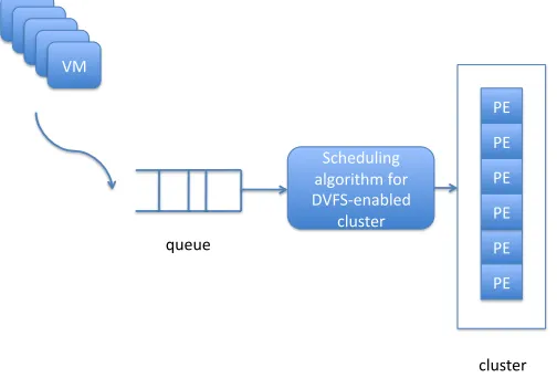
Fig. 3. Working scenario of a DVFS-enabled cluster scheduling

sorted in a queue. Algorithm 1 shows the scheduling algorithm for virtual machines in a DVFS-enabled cluster. A scheduling algorithm runs as a daemon in a cluster with a predefined schedule interval,INTERVAL. During the period of scheduling interval, incoming virtual machines arrive at the scheduler and will be scheduled at the next schedule round.Fj,1≤j≤J is

a set of PEs that run in the operating point ofopj. Firstly the

Algorithm 1 sets F1, F2, ..., FJ with empty sets (line 1). The

wall clock time,t, is initialized with0. Algorithm 1 initializes all PEs as follows (line 2 – 6):

• set all PEs running to the lowest voltage and processor

speed,smin;

• pek.sa is defined as the available processor speed if

the processor does not change its operating point. Since no virtual machine are initially scheduled, pek.sa is

initialized withsmin;

• pek.∇sis the available PE processor speed whenpek is

operated to a highest level voltage from current voltage level. pek.∇s is initialized withsmax.

The scheduler iterates (line 8) with a predefined interval value, INTERVAL, from starting time 0; In each scheduling round, the scheduler firstly levels down power profiles of PEs. The reason is that some virtual machines might finish its exe-cution during the last scheduling round and some PEs are no longer needed to be operated in high voltages. Then the power profiles of some PEs are leveled down. Then the scheduler places incoming virtual machines in the queue to PEs while minimizing the power consumption with Algorithm 2. The scheduler sleeps during the schedule period, INTERVAL.

Algorithm 2 is used to schedule incoming virtual machine requests in a certain schedule round. The Algorithm 2 sorts the incoming virtual machine requests in decreasing order of required processing frequency, vmi.sr, (line 1). Virtual

ma-chines with more resource requirement,vmi.sr, are scheduled

in higher priorities. If there are unscheduled virtual machines in the last schedule round, they are set in the highest priorities. Lines 2 – 27 of Algorithm 2 describe the process to schedule all the incoming virtual machine requests. For each virtual machinevmi(line 2), the Algorithm 2 checks the PE operating

Algorithm 2 Scheduling VMs in an interval of Algorithm 1

1: Sort vmi ∈ V M in a decreasing order of their required

processor speed,vmi.sr.

If there are some unscheduled virtual machines in the last schedule round, put them in front of the virtual machine set

V M.

2: FORi= 1 TOi≤I DO 3: FOR j= 1TOj≤J DO

4: findpen∈Fj which has the max pen.sa

5: IF pen.sa ≥vmi.sr THEN

6: schedulevmi onpen

7: pen.sa =pen.sa−vmi.sr

8: pen.∇s=pen.∇s−vmri

9: go to schedulevmi+1

10: END IF 11: END FOR

12: IFvmi is not scheduled THEN

13: find pen, which has the max pen.∇s

14: IF pen.∇s≥vmi.sr THEN

15: j=pen.oppe

16: movepen fromFj toFk,opk is the lowest possible

voltage level that can schedulevmi,j < k≤J.

17: pen.spe=opk.sop

18: pen.vpe=opk.vop

19: pen.oppe=k

20: schedulevmi onpen

21: pen.sa =pen.sa+ (opk.sop−opj.sop)−vmi.sr

22: pen.∇s=pen.sa+ (smax−opk.sop)−vmi.sr

23: ELSE

24: vmi cannot be scheduled now;

it will be rescheduled at next turn. 25: END IF

26: END IF 27: END FOR

point set, OP, from low voltage level to high voltage level (line 3). In the PE set with lowest possible voltage level, it finds the PE with the maximum available processor speed,

pen.sa. If this PE can fulfill the virtual machine requirement

, vmi.sr, which is pen.sa > vmi.sr in line 5, vmi can be

scheduled on this PE,pen. This means current voltage profile

can schedule the incoming virtual machinevmi and no PE is

required to updated to a higher voltage.

If no PE can schedule the virtual machine vmi (line 12),

certain PE should be operated with higher voltage. The Algo-rithm 2 selects the PE with the maximum potential processor speedpen.∇s (line 13). If this PE can fulfill the requirement

of vmi (pen.∇s ≥ vmi.sr), the Algorithm 2 then operates

this PE in a higher voltage level and schedules vmi on this

PE. In detail, the Algorithm 2 locates the lowest possible voltage levelk, which is higher than current voltage level j,

scheduling virtual machine vmi (line 14). Then Algorithm 2

schedules the virtual machinevmi on this PEpen and update

related information (line 14 – 23). If no PE can schedule the virtual machine vmi even all PEs are operated in the highest

voltage level, the Algorithm 2 returns information that vmi

cannot be scheduled at current scheduling round.

Algorithm 3Level down VM voltage profiles in a scheduling

round

1: FOR i= 1toI DO

2: IFt−vmi.tr≥vmi.∆t THEN

3: setvmi finished its execution onpen∈Fj

4: pen.sa=pen.sa+vmi.sr

5: pen.∇s=pen.∇s+vmi.sr

6: ENDIF

7: FOR j=J TO 2 DO 8: FOR pen ∈Fj DO

9: level down pen to the operating point set Fk with

lowest possible voltage,1≤k < j, ifopk.sop can support all

current virtual machines on pen

10: ENDFOR

After one schedule interval passes, some virtual machines may have finished their execution. Therefore we have defined Algorithm 3 to reduce a number of PE’s supply voltages if they are not fully utilized. Algorithm 3 first checks whether virtual machines have finished their execution (line 2). For those PEs whose virtual machines have finished, the PE information such as available processor speed, pen.sa, and and maximum

potential processor speed, pen.∇s, are updated (line 4, 5).

Then Algorithm 3 checks all PEs that run on high voltages, and try to level down their operating points without affecting virtual machines that run on them (line 9).

VI. PERFORMANCEEVALUATION IN AMULTICORE

CLUSTER

In order to validate our model and scheduling algorithm, it is important to investigate the feasibility within a real virtual machine cluster environment. This section discusses the implementation of our scheduling algorithm as it is applied to the OpenNebula project in a multi-core cluster. The following experiments in this section help derive the parameters for our simulation later in Section VII.

A. Implementation in OpenNebula

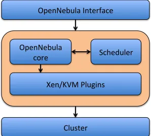
OpenNebula [31] is an open source distributed virtual machine manager for dynamic allocation of virtual machines in a resource pool, such as a compute cluster. Figure 4 shows the software architecture of OpenNebula. The OpenNebula core components accept user requirements via the OpenNebula interface, and then place virtual machines in compute nodes within the cluster.

From Figure 4 we see the OpenNebula scheduler is an inde-pendent component that provides policies for virtual machine placement. We choose the OpenNebula project because of this

Cluster
 Xen/KVM
Plugins


Scheduler
 OpenNebula


core


OpenNebula
Interface


Fig. 4. OpenNebula Software Architecture

compartmentalized design as it allows us to easily integrate our custom scheduling algorithm. The default scheduler provides a rank scheduling policy, which allocates compute resources for virtual machines based on resource ranks. Scheduling algorithms 1 - 3 are implemented by modifying the Open-Nebula scheduler to reflect the desired results in Section V. As such, we implement a loose interpretation of the algorithms to provide a power-aware scheduling system for the OpenNebula platform.

In order to accomplish this task, we must take advantage of power management techniques at they hypervisor level. For our implementation, we do this through the use of the Xen Hypervisor. Xen, in specific version 3.3.4, allows for the frequency to be adjusted based on available P-states within the Dom0 Operating System using thexenpmcommand [32], [33]. By default, Xen uses a performance governor which keeps all CPU frequencies at the highest setting. For the following experiments, we set the governor to userspace to enable manual control of the frequencies as desired.

In order to test our design, we created a two-node ex-perimental multi-core cluster consisting of Intel Nehalem quad-core processors with Hyperthreading (providing 8 virtual cores). The Nehalem-based CPUs allow for each core to op-erate on its own independent P-state, thereby maximising the frequency scaling flexibility. The compute nodes are installed with Ubuntu Server 8.10 with Xen 3.3.4-unstable. The head node consists of a Pentium 4 CPU installed with Ubuntu 8.10, OpenNebula 1.2 and a NFS server to allow compute nodes access to OpenNebula files and VM images.

B. Experiment and Test Results

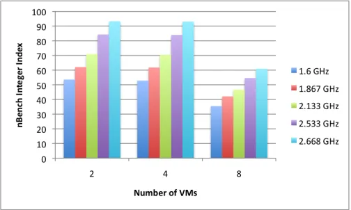
For this experiment, we schedule all virtual machines to the compute nodes and run the nBench [34] Linux Benchmark ver-sion 2.2.3 to approximate the system performance. The nBench application is an ideal choice as it is easily compiled in Linux, combines a number of different mathematical applications to evaluate performance, and it provides a comparable Integer and Floating Point Index that can used to evaluate overall system performance. The operating frequency of each core can be set to 1.6Hz, 1.86Ghz, 2.13GHz, 2.53GHz, or 2.66Ghz, giving the processor a frequency range of over 1.0 Ghz.

Fig. 5. Power consumption variations for a Intel Nehalem Quad-core processor

and 8 VMs at each frequency while computing the nBench Linux Benchmark. Here the benchmark effectively simulates a CPU-intensive job running within a VM and provides valuable information on the performance of each VM.

There are a number of things that can be observed from Figure 5. First, while scheduling more virtual machines on a node raises power consumption, it seems to consume far less power than operating two separate nodes. Therefore, it seems logical for a scheduler to run as many virtual machines on a node as possible until all available virtual CPUs are taken. Second, when the frequency is dynamically reduced, the difference between running nBench on 2 VMs versus 8 VMs at 1.6GHz is only 28.3 Watts. When running the benchmark at 2.668 GHz (the maximum frequency available), this difference grows to 65.2 Watts, resulting in a larger VM power consumption difference and also a larger overall power consumption of 209 Watts.

It would be desirable to run each core at its lowest voltage 100% of the time to minimise power consumption, however one must consider the performance impact of doing so. In Figure 6 the average nBench Integer calculation Index is illustrated with the number of VMs per node and operating frequency dynamically varied for each test.

Fig. 6. Performance impact of varying the number of VMs and operating frequency

Figure 6 illustrates how the performance degradation due

to operating frequency scaling is a linear relationship. This eliminates any question of unexpected slowdowns in perfor-mance when running at frequencies lower than the maximum, such as 1.6GHz. Another interesting observation is the node’s performance running 8 VMs. Due to Intel’s Hyperthreading technology, the CPU reports as 8 virtual cores within the host OS (Dom0) even though there are really only 4 cores per node. In our case of running nBench on virtual machines, theres seems to be an overall increased throughput by using 8 VMs instead of just 4. While the performance of each individual VM is only approximately 67% as fast when using 8 VMs instead of 4, there are twice as many VMs to contribute to an overall performance improvement of 34%, which is consistent with previous reports [35] of optimal speedups when using Hyperthreading. Therefore its even more advisable to schedule as many virtual machines on one physical node because it maximises not only power consumption per VM, but also overall system performance.

VII. PERFORMANCESTUDYWITHSIMULATION

While it would be ideal to deploy such a system as described in Section VI in a real data center, such a task is not feasible at this time. Instead we create a simulator named DVFS-SIM to simulate the algorithm in DVFS-enabled clusters by enabling DVFS functionalities in the processor performance model. The goal of this simulator is to illustrate the usefulness of our model and algorithm so as to justify the model’s deployment on a large-scale cluster system.

A. Implementation of DVFS-SIM

The design of DVFS-SIM consists of the following mod-ules:

• Job module: The job module is developed to simulate various jobs to be executed in a cluster. Virtual machines are modeled as incoming jobs with required processor speed and execution time as parameters.

• Cluster module:The cluster module is presented to simu-late a deployed cluster environment in use today, such as the IKEP cluster. It is represented by a node configuration and scheduling algorithm implementation. A scheduler runs as a daemon to accept and handle incoming jobs.

• PE module: The DVFS performance model is

imple-mented in the PE Module. Each PE loops at a defined interval to simulate a specific processor operating fre-quency.

We simulate the scheduling algorithm with 10, 20, 30, 40, and 50 compute nodes. Multiple virtual machines are generated in the job module. We simulate 100, 200, 300, 400 and 500 virtual machines. To satisfy the cluster module described above, the Virtual machine resource requirements are randomly generated in the range of 0.1 GHz – 1.0 GHz and required execution times are randomly generated in the range of 1.0 time unit – 10.0 time unit.

following previous work from [28] as an example and to allow for the comparison of research results in a meaningful and fair way.

Table I shows the operating points of the Pentium M 1.4 GHz simulated for this performance study.

TABLE I

OPERATING POINTS FOR THEPENTIUMM 1.4 GHZ PROCESSOR

Frequency (GHz) Supply Voltage (V)

1.4 1.484

1.2 1.436

1.0 1.308

0.8 1.180

0.6 0.956

B. Simulation Results

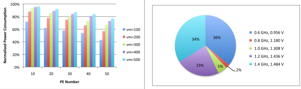
Figure 7 shows simulation results for DVFS-enabled cluster scheduling algorithm (Algorithms 1 – 3). The X-axis is the number of PEs and the Y-axis is the normalized power consumption. The base for normalization is the power con-sumption when all PEs are operated in the highest voltage. Looking at this data, we canmake the following observations:

• Observation 1: The scheduling algorithm can reduce power consumption in a DVFS-enabled cluster.

• Observation 2:In case that the number of PEs is fixed, the power consumption increases as the number of incoming virtual machines increases.

• Observation 3: In case that the number of incoming vir-tual machine is fixed, the power consumption decreases as the number of PEs increases.

!"# $!"# %!"# &!"# '!"# (!!"#

(!# $!# )!# %!# *!#

!"#$%&'(

)*+,

"-)#+."/01$23"/+

,4+!1$5)#+

+,-(!!# +,-$!!# +,-)!!# +,-%!!# +,-*!!#

Fig. 7. DVFS-enabled cluster scheduling simulation results

We interpret the simulated behavior as follows. For Obser-vation 1, in the operation of a DVFS-enabled cluster some PEs operate with lower voltages. Thus, compared with a fully utilized cluster using the highest voltages, less power is consumed. Observation 2 can be interpreted as when more virtual machines arrive in a cluster, the PEs of the cluster are forced to operate with higher voltages to provide more processing capacities, thus requiring more power consumption.

On the contrary, when more PEs are available for a fixed number of incoming virtual machines, the PEs could be operated with lower voltages since enough PEs are provided leading to Observation 3 where less power consumption is observed.

!" #" $!" $#" %!" %#" &!" &#" '!"

$" %" &" '" #"

!"#$%&'()#

*+,(-%.(#)/%$-#

!()"*+,-"!(.#)"/" !(0"*+,-"$($0!"/""" $(!"*+,-"$(&!0"/" $(%"*+,-"$('&)"/" $('"*+,-"$('0'"/"

Fig. 8. Operating point distribution with schedule rounds (VM No. = 200, PE No. = 40)

Figure 8 shows the distribution of sample PE operating frequencies when 200 virtual machines are scheduled in a cluster with 40 PEs. When scheduling first starts in Algorithm 3, the PEs are operated with a low frequency and voltage (0.6 GHz, 0.956V) because enough PEs are available. When more incoming virtual machine requests arive to be scheduled on the cluster, PEs are loaded with more virtual machines and in turn are operated with higher frequencies and voltages. In this scenario, the number of PEs operated at 1.4 GHz increases and the number of PEs operated with 0.6 GHz decreases. Figure 9 shows the overall operation point distribution during the whole scheduling process.

!"#$

%#$ &#$ %!#$ !'#$

()"$*+,-$().&"$/$ ()0$*+,-$1)10($/$ 1)($*+,-$1)!(0$/$ 1)%$*+,-$1)'!"$/$ 1)'$*+,-$1)'0'$/$

Fig. 9. Overall operating point distribution (VM No.= 200, PE No.= 40)

C. Discussion

• The simulated and experimental CPU architectures are too different to compare. The Pentium M is a mobile chipset that is over 4 years old, while the Intel Nehalem is a multi-core chipset that is is less than 6 months old.

• The simulation did not take into account the overhead

introduced by the OpenNebula project. The differences could be a manifestation of the scheduling delay, the image transferring and access through NFS, newtork latency, all of which could lead to differences in power consumption.

• The simulation did not take into account a host hypervisor OS. In the experimental case, this consisted of a Ubuntu Linux Dom0 installation which could add delays and increased power consumption.

VIII. CONCLUSION ANDFUTUREWORK

As the computing industry continues to consolidate indi-vidual servers into large data centers using Cloud computing technologies, the need for efficient algorithms to minimize wasted server energy becomes increasingly important. As such, the field of Green computing provides a way to pre-vent unnecessaryCO2 emissions from contributing to Global

Warming and to save large amounts of money on operating costs.

Future work includes the deployment of the power aware scheduling algorithm in production clusters, for example IKEP cluster, the analysis and measuring of virtual machine migra-tion costs in a cluster, and the development of a temperature-aware scheduling algorithms for multi-core compute clusters.

REFERENCES

[1] A. Gara, M. A. Blumrich, D. Chen, G. L.-T. Chiu, P. Coteus, M. Gi-ampapa, R. A. Haring, P. Heidelberger, D. Hoenicke, G. V. Kopcsay, T. A. Liebsch, M. Ohmacht, B. D. Steinmacher-Burow, T. Takken, and P. Vranas, “Overview of the Blue Gene/L system architecture,” IBM Journal of Research and Development, vol. 49, no. 2-3, pp. 195–212, 2005.

[2] K. Li, “Performance Analysis of Power-Aware Task Scheduling Algo-rithms on Multiprocessor Computers with Dynamic Voltage and Speed,”

IEEE Trans. Parallel Distrib. Syst., vol. 19, no. 11, pp. 1484–1497, 2008.

[3] W. Forrest, “How to cut data centre carbon

emissions?” Website, December 2008. [Online]. Available:

http://www.computerweekly.com/Articles/2008/12/05/233748/how-to-cut-data-centre-carbon-emissions.htm

[4] P. W. Hale, “Acceleration and time to fail,” Quality and Reliability Engineering International, vol. 2, no. 4, pp. 259–262, 1986.

[5] G. Magklis, G. Semeraro, D. Albonesi, S. Dropsho, S. Dwarkadas, and M. Scott, “Dynamic frequency and voltage scaling for a multiple-clock-domain microprocessor,”IEEE Micro, vol. 23, no. 6, pp. 62–68, 2003. [6] L. Wang, M. Kunze, and J. Tao, “Performance evaluation of virtual machine based Grid workflow system,”Concurrency and Computation: Practice and Experience, vol. 20, no. 15, pp. 1759–1771, 2008. [7] W. Huang, J. Liu, B. Abali, and D. K. Panda, “A case for high

performance computing with virtual machines,” inProceedings of the 20th Annual International Conference on Supercomputing, 2006, pp. 125–134.

[8] V. B¨uge, Y. Kemp, M. Kunze, and G. Quast, “Application of Virtuali-sation Techniques at a University Grid Center,” ine-Science, 2006, p. 155.

[9] N. Fallenbeck, H. Picht, M. Smith, and B. Freisleben, “Xen and the art of cluster scheduling,” inFirst International Workshop on Virtualization Technology in Distributed Computing, 2006, pp. 4–4.

[10] Y. Wiseman and D. Feitelson, “Paired gang scheduling,”IEEE Transac-tions on Parallel and Distributed Systems, vol. 14, no. 6, pp. 581–592, 2003.

[11] C.-H. Hsu and W. chun Feng, “A Feasibility Analysis of Power Aware-ness in Commodity-Based High-Performance Clusters,” inCLUSTER, 2005, pp. 1–10.

[12] C. Hsu and W. Feng, “A power-aware run-time system for high-performance computing,” inProceedings of the 2005 ACM/IEEE con-ference on Supercomputing. IEEE Computer Society Washington, DC, USA, 2005.

[13] I. Gorton, Greenfield, P., Szalay, A., and R. Williams, “Data-Intensive Computing in the 21st Century,” IEEE Computer, vol. 41, no. 4, pp. 30–32, 2008.

[14] W. Feng, A. Ching, C. Hsu, and V. Tech, “Green Supercomputing in a Desktop Box,” in IEEE International Parallel and Distributed Processing Symposium, 2007. IPDPS 2007, 2007, pp. 1–8.

[15] W. Feng and K. Cameron, “The Green500 List: Encouraging Sustainable Supercomputing,”IEEE Computer, pp. 50–55, 2007.

[16] W. Feng and X. Feng, “Green supercomputing comes of age,” IT Professional, vol. 10, no. 1, pp. 17–23, 2008.

[17] D. Bodas, “Data Center Power Management and Benefits to

Modular Computing,” in Intel Developer Forum, 2003. [Online]. Available: http://www.intel.com/idf/us/spr2003/presentations/S0 3US-MODS137 OS.pdf

[18] G. Chen, K. Malkowski, M. Kandemir, and P. Raghavan, “Reducing power with performance constraints for parallel sparse applications,” in

19th IEEE International Parallel and Distributed Processing Sympo-sium, 2005. Proceedings, 2005, p. 8.

[19] V. Freeh and D. Lowenthal, “Using multiple energy gears in MPI programs on a power-scalable cluster,” in Proceedings of the tenth ACM SIGPLAN symposium on Principles and practice of parallel programming. ACM New York, NY, USA, 2005, pp. 164–173. [20] R. Ge, F. X., F. W., and K. Cameron, “CPU MISER: A

Performance-Directed, Run-Time System for Power-Aware Clusters,” inProceedings of the 2007 International Conference on Parallel Processing. IEEE Computer Society Washington, DC, USA, 2007.

[21] J. Smith and R. Nair,Virtual machines: versatile platforms for systems and processes. The Morgan Kaufmann, 2003.

[22] R. J. O. Figueiredo, P. A. Dinda, and J. A. B.

Fortes, “A case for grid computing on virtual machine,”

in ICDCS, 2003, pp. 550–559. [Online]. Available: http://csdl.computer.org/comp/proceedings/icdcs/2003/1920/00/19200550abs.htm [23] CERN, “LHC Computing Grid Project,” Web Page, Dec. 2003.

[Online]. Available: http://lcg.web.cern.ch/LCG/

[24] “CDF,” Web Page. [Online]. Available: http://www/cdf.fnal.gov/ [25] “CMS,” Web Page. [Online]. Available: http://cms.cern.ch/

[26] J. Luo, A. Song, Y. Zhu, X. Wang, T. Ma, Z. Wu, Y. Xu, and L. Ge, “Grid supporting platform for AMS data processing,”Lecture notes in computer science, vol. 3759, p. 276, 2005.

[27] K. H. Kim, R. Buyya, and J. Kim, “Power Aware Scheduling of Bag-of-Tasks Applications with Deadline Constraints on DVS-enabled Clusters,” inCCGRID, 2007, pp. 541–548.

[28] R. Ge, X. Feng, and K. Cameron, “Performance-constrained distributed dvs scheduling for scientific applications on power-aware clusters,” in

Proceedings of the 2005 ACM/IEEE conference on Supercomputing. IEEE Computer Society Washington, DC, USA, 2005.

[29] J. Li and J. F. Mart´ınez, “Dynamic power-performance adaptation of parallel computation on chip multiprocessors,” inHPCA, 2006, pp. 77– 87.

[30] C. Piguet, C. Schuster, and J. Nagel, “Optimizing architecture activity and logic depth for static and dynamic power reduction,” inCircuits and Systems, 2004. NEWCAS 2004. The 2nd Annual IEEE Northeast Workshop on, 2004, pp. 41–44.

[31] J. Fontan, T. Vazquez, L. Gonzalez, R. S. Montero, and I. M. Llorente, “OpenNEbula: The Open Source Virtual Machine Manager for Cluster Computing,” in Open Source Grid and Cluster Software Conference, San Francisco, CA, USA, May 2008.

[32] G. Wei, J. Liu, J. Xu, G. Lu, K. Yu, and K. Tian, “The On-going Evolutions of Power Management in Xen,” Intel Corporation, Tech. Rep., 2009.

[33] K. Yu, “Xen PM,” Website, March 2009. [Online]. Available: http://wiki.xensource.com/xenwiki/xenpm

[34] Webpage, May 2008. [Online]. Available: http://www.tux.org/ may-er/linux/bmark.html

[35] D. Marr, F. Binns, D. Hill, G. Hinton, D. Koufaty, J. Miller, and M. Up-ton, “Hyper-threading technology architecture and microarchitecture,”